Discretionary Lane-Change Decision and Control via Parameterized Soft Actor–Critic for Hybrid Action Space

Abstract

This study focuses on a crucial task in the field of autonomous driving, autonomous lane change. Autonomous lane change plays a pivotal role in improving traffic flow, alleviating driver burden, and reducing the risk of traffic accidents. However, due to the complexity and uncertainty of lane-change scenarios, the functionality of autonomous lane change still faces challenges. In this research, we conducted autonomous lane-change simulations using both deep reinforcement learning (DRL) and model predictive control (MPC). Specifically, we used the parameterized soft actor–critic (PASAC) algorithm to train a DRL-based lane-change strategy to output both discrete lane-change decisions and continuous longitudinal vehicle acceleration. We also used MPC for lane selection based on the smallest predictive car-following costs for the different lanes. For the first time, we compared the performance of DRL and MPC in the context of lane-change decisions. The simulation results indicated that, under the same reward/cost function and traffic flow, both MPC and PASAC achieved a collision rate of 0%. PASAC demonstrated a comparable performance to MPC in terms of average rewards/costs and vehicle speeds.

1. Introduction

The development of autonomous driving has indeed brought revolutionary changes to transportation [1]. Autonomous driving technology not only alleviates the burden on drivers and improves traffic flow but, more importantly, it significantly reduces traffic accidents caused by human errors when driving. According to the World Health Organization, nearly 1.3 million people die in road traffic accidents globally each year, with 94% attributed to driver errors. In lane-change scenarios in particular, the actions of surrounding vehicles are often challenging to predict, making automated lane-change a critical task for autonomous vehicles.

Research has indicated that nearly 10% of highway accidents are caused by lane-change maneuvers [2]. Therefore, a safe, smooth, and efficient automated lane-change mechanism is crucial for autonomous vehicles. To achieve this goal, the vehicle’s architecture must possess efficient and robust execution capabilities that are able to handle uncertainties in the operating environment, make rational decisions, and execute appropriate actions to cope with the potentially adversarial or cooperative behaviors of surrounding vehicles.

Currently, automated lane changing in autonomous driving is considered Level 2 automation [3]. Advanced driver-assistance systems such as lane keeping assist (LKA), lane centering control (LCC), and adaptive cruise control (ACC) [4] are relatively well-established, but the lane-change function still requires further development and improvement. Although there has been some progress in research in automated lane-change decision-making, this functionality has not yet been widely implemented in vehicles.

MPC stands out as a method of optimizing a sequence of future control actions to address real-time control problems. For instance, Ji proposed a collision-free trajectory planning method based on artificial potential fields and multi-constraint MPC [5]. Raffo presented an MPC-based trajectory tracking method, with two cascaded MPC controllers handling vehicle kinematics and dynamics models, effectively reducing computational complexity [6]. Xu introduced an MPC controller for a lane-keeping system, utilizing a five-point interpolation method to generate a reference trajectory [7]. Similarly, Sameul conducted simulations comparing MPC and PID controllers for trajectory tracking in autonomous vehicles, finding that MPC exhibited better robustness in various scenarios, including vehicle load, longitudinal velocity, and steering changes [8]. Hang proposed a human-like decision-making framework, combining potential field methods and MPC for collision-free path planning. Additionally, he introduced a module that integrated decision-making and motion planning, considering the social behavior of surrounding traffic participants [9,10].

On the other hand, reinforcement learning (RL) has consistently been a research hotspot in the field of decision-making. For instance, the AlphaGo Go-playing robot, which defeated the human Go champion, was a result of training in discrete-action reinforcement learning [11]. Currently recognized discrete-action reinforcement learning algorithms include the Deep Q-Network (DQN) [10], Double DQN (DDQN) [12], and Rainbow [13], among others. Continuous-action reinforcement learning algorithms include the Deep Deterministic Policy Gradient (DDPG) [14], Twin-Delayed DDPG (TD3) [15], Soft Actor Critic (SAC) [16], and so on.

Few papers have proposed different methods for obtaining hybrid action spaces [17]. One highly cited method is parameterized DDPG (PA-DDPG), introduced in 2016 by scholars from the University of Texas, which utilizes continuous-action reinforcement learning to address hybrid action spaces [18]. Another well-cited method is the Parameterized Deep Q-Network (PDQN), proposed in 2018 by researchers from Tencent AI Lab, which combines actor–critic learning and Q-learning, utilizing Q-learning instead of critic learning in DDPG for discrete action selection [19]. In 2019, scholars from the University of Twente proposed an improved approach called multi-pass P-DQN (MPDQN) [20], which distributes continuous action inputs to the Q-network based on the correspondence between discrete and corresponding continuous actions, resulting in more reasonable Q-value outputs. In 2022, scholars from Tianjin University introduced the HyAR-TD3 algorithm [21], which employs representation learning to map continuous action spaces and hybrid action spaces.

Currently, most literature uses discrete reinforcement learning to achieve optimal control for non-mandatory automated lane changing of autonomous vehicles [22,23,24,25,26]. Typically, these papers adopt a hierarchical control approach, where the upper-level control outputs lane-change decisions using discrete reinforcement learning (discrete control variables), and the lower-level control uses a car-following model to output the vehicle acceleration (continuous control variables). However, only a few studies have applied hybrid-action reinforcement learning to automated lane-change decision-making and control. In 2021, scholars from the University of Washington proposed the Hybrid Deep Q-Learning and Policy Gradient (HDQPG) to achieve automated lane-change of vehicles [27].

In this paper, we use the PASAC algorithm tailored for hybrid-action spaces. We trained the model using traffic simulation software on the SUMO platform for various traffic scenarios. To validate the algorithm’s superior performance in terms of stability and optimality, we compared the results of PASAC with MPC, considering metrics such as collision rate, average speed, value function, and jerk. However, it is crucial to note some known differences between the two approaches. First, MPC requires online optimization and demands relatively powerful computing resources for real-time applications, raising monetary concerns about practical deployment [28]. On the other hand, the DRL solution, based on neural networks, despite being time-consuming during offline training, has short execution times and is suitable for real-time applications. Second, MPC relies on a model-based approach, while DRL control solutions, based on black-box neural networks, lack theoretical guarantees [29].

In our MPC model, the ego vehicle needs to assess whether executing a lane-change maneuver is beneficial. If deemed beneficial, it adjusts its position and speed to prepare for the lane change; otherwise, it chooses to follow the preceding vehicle. In RL, the intelligent agent interacts with the environment, selects actions based on the current state, and continually updates its policy based on environmental feedback in the form of rewards. The intelligent agent in reinforcement learning can learn adaptive driving strategies for lane-change problems, enabling vehicles to make intelligent lane-change decisions.

The primary contribution of this work is the introduction of the PASAC algorithm for discretionary lane changing, as well as the first quantitative and comprehensive comparison of the hybrid-action space reinforcement learning algorithm PASAC with MPC. We experimentally verified the superiority of PASAC in lane-change decision and control, and conducted a detailed analysis of its performance. To the best of our knowledge, such a comparison does not exist in the literature. This not only provides new insights into the application of hybrid-action space reinforcement learning in practical control problems but also offers empirical support for the comparison of reinforcement learning with traditional control methods.

Regarding the structure of this paper, the Section 2 provides a detailed introduction to the PASAC algorithm. The application of PASAC and MPC in lane-change scenarios is discussed in the Section 3 and Section 4, respectively. The Section 5 compares the DRL and MPC methods. Finally, conclusions are drawn in the sixth section.

2. Parameterized Soft Actor–Critic

In this section, we present an overview of the hybrid action space structure using the SAC algorithm.

2.1. Reinforcement Learning

Reinforcement learning is a learning method employed for decision-making and control. In reinforcement learning, an agent takes actions based on the current time step’s environmental state, and subsequently, the environment transitions to a new state in the next time step as a result of that action. The agent also receives rewards based on the actions taken, and both the actions and rewards have a certain probabilistic nature. The objective of reinforcement learning algorithms is to learn effective policies by maximizing the expected discounted cumulative reward for each episode. Specifically, the discounted cumulative reward for a state-action pair is referred to as the Q-value, denoted as $Q({\mathbf{s}}_t,{\mathbf{a}}_t)=\mathbb{E}{[}_{\tau =t}^{\tau =T}{\gamma }^{\tau -T}r\left({\mathbf{s}}_{\tau },{\mathbf{a}}_{\tau }\right)]$. Here, $r\left({\mathbf{s}}_{\tau },{\mathbf{a}}_{\tau }\right)$ represents the reward for the state s and action a at time step $\tau$, and $\gamma \in$ [0, 1] is the discount factor. The resolution of reinforcement learning problems adheres to the Bellman optimality principle. This principle asserts that if the optimal Q-value for the next step is known, then the action for the current time step must also be optimal. In other words, for an optimal policy, $Q{({\mathbf{s}}_t,{\mathbf{a}}_t)}^{\ast }=r({\mathbf{s}}_t,{\mathbf{a}}_t)+\gamma Q^{\ast }({\mathbf{s}}_{t+1},{\mathbf{a}}_{t+1})$, with ∗ denoting the optimality. This principle forms the foundation for devising effective policies in reinforcement learning.

2.2. Soft Actor–Critic

The actor–critic architecture is a core component of the RL algorithm, as proposed by Sutton and Barto (1999) [30]. It is used to solve action selection and value function learning. In this context, we consider a parameterized state value function V, a soft Q function, and a policy network. The parameters of these networks are denoted as $\psi$, $\widehat{\psi }$, $\theta$, and $\varphi$, respectively. The SAC algorithm considers the maximum entropy objective in reinforcement learning’s maximum expectation, and the modified expectation is

$$J\left(\pi \right)=\sum _{t=0}^T{\mathbb{E}}_{({\mathbf{s}}_t,{\mathbf{a}}_t)\sim {\rho }_{\pi }}{\gamma }^t\left[r({\mathbf{s}}_t,{\mathbf{a}}_t)+\alpha H\left(\pi (·|{\mathbf{s}}_t)\right)\right],$$

(1)

In this formula, “·” represents all possible actions. ${\rho }_{\pi }$ denotes the new policy. The higher the entropy H, the stronger the system’s uncertainty. In other words, a policy with higher entropy provides more significant action unpredictability. To regulate the impact of entropy on the policy, the SAC algorithm introduces a hyperparameter $\alpha$, which plays a pivotal role in determining the relative significance of the entropy term on rewards.

$${\pi }^{\ast }=arg\underset{\pi }{max}\mathbb{E}\underset{\tau \sim \pi }{\phantom{.}}\left[\sum _{t=0}^{\infty }{\gamma }^t\left(R({\mathbf{s}}_t,{\mathbf{a}}_t,{\mathbf{s}}_{t+1})\right)+\alpha H\left(\pi (·|{\mathbf{s}}_t)\right)\right],$$

(2)

The primary objective in training the soft value function is to minimize the square of residuals. In essence, through the optimization of the soft value function, the goal is to diminish the disparity between model predictions and actual observations, thereby enhancing the overall efficacy of the training process.

$$J_V\left(\psi \right)={\mathbb{E}}_{s_t\sim D}\left[\frac{1}{2}{(V_{\psi }\left({\mathbf{s}}_t\right)-E_{{\mathbf{a}}_t\sim {\pi }_{\psi }}[Q_{\theta }({\mathbf{s}}_t,{\mathbf{a}}_t)-log{\pi }_{\varphi }\left({\mathbf{a}}_t\right|{\mathbf{s}}_t)])}^2\right],$$

(3)

The gradient can be estimated using an unbiased estimator

$${\widehat{▽}}_{\psi }{J}_V\left(\psi \right)={▽}_{\psi }{V}_{\psi }\left({\mathbf{s}}_t\right)(V_{\psi }\left({\mathbf{s}}_t\right)-Q_{\theta }({\mathbf{s}}_t,{\mathbf{a}}_t)+log{\pi }_{\varphi }\left({\mathbf{a}}_t\right|{\mathbf{s}}_t)),$$

(4)

The parameters of the soft Q-value function are determined by minimizing the residual of the Bellman equation.

$$J_Q\left(\theta \right)={\mathbb{E}}_{({\mathbf{s}}_t,{\mathbf{a}}_t)\sim D}\left[\frac{1}{2}{\left(Q_{\theta }({\mathbf{s}}_t,{\mathbf{a}}_t)-\widehat{Q}({\mathbf{s}}_t,{\mathbf{a}}_t)\right)}^2\right],$$

(5)

with

$$\widehat{Q}({\mathbf{s}}_t,{\mathbf{a}}_t)=r({\mathbf{s}}_t,{\mathbf{a}}_t)+\gamma {\mathbb{E}}_{s_t\sim p}\left[V_{\widehat{\psi }}\left(s_{t+1}\right)\right],$$

(6)

After optimizing with a stochastic gradient

$${\widehat{▽}}_{\theta }{J}_Q\left(\theta \right)={▽}_{\theta }{Q}_{\theta }({\mathbf{s}}_t,{\mathbf{a}}_t)(Q_{\theta }({\mathbf{s}}_t,{\mathbf{a}}_t)-r({\mathbf{s}}_t,{\mathbf{a}}_t)-\gamma V_{\widehat{\psi }}\left(s_{t+1}\right)),$$

(7)

The method of translating strategies using neural networks is as follows:

$${\mathbf{a}}_t=f_{\varphi }({ϵ}_t;{\mathbf{s}}_t),$$

(8)

${ϵ}_t$ represents an input noise vector sampled from a fixed distribution, such as a spherical Gaussian distribution.The objective function is denoted as

$$J_{\pi }\left(\varphi \right)={\mathbb{E}}_{s_t\sim D,{ϵ}_t\sim N}\left[log{\pi }_{\varphi }\left(f_{\varphi }({ϵ}_t;{\mathbf{s}}_t)\right|s_t)-Q_{\theta }({\mathbf{s}}_t,f_{\varphi }({ϵ}_t;{\mathbf{s}}_t))\right],$$

(9)

where ${\pi }_{\varphi }$ is defined by the function $f_{\varphi }$, the gradient of Equation (9) is as follows:

$${\widehat{▽}}_{\varphi }{J}_{\pi }\left(\varphi \right)={▽}_{\varphi }log{\pi }_{\varphi }\left({\mathbf{a}}_t\right|{\mathbf{s}}_t)+({▽}_{{\mathbf{a}}_t}log{\pi }_{\varphi }\left({\mathbf{a}}_t\right|{\mathbf{s}}_t)-{▽}_{{\mathbf{a}}_t}Q({\mathbf{a}}_t,{\mathbf{s}}_t)){▽}_{\varphi }{f}_{\varphi }(ϵ;{\mathbf{s}}_t).$$

(10)

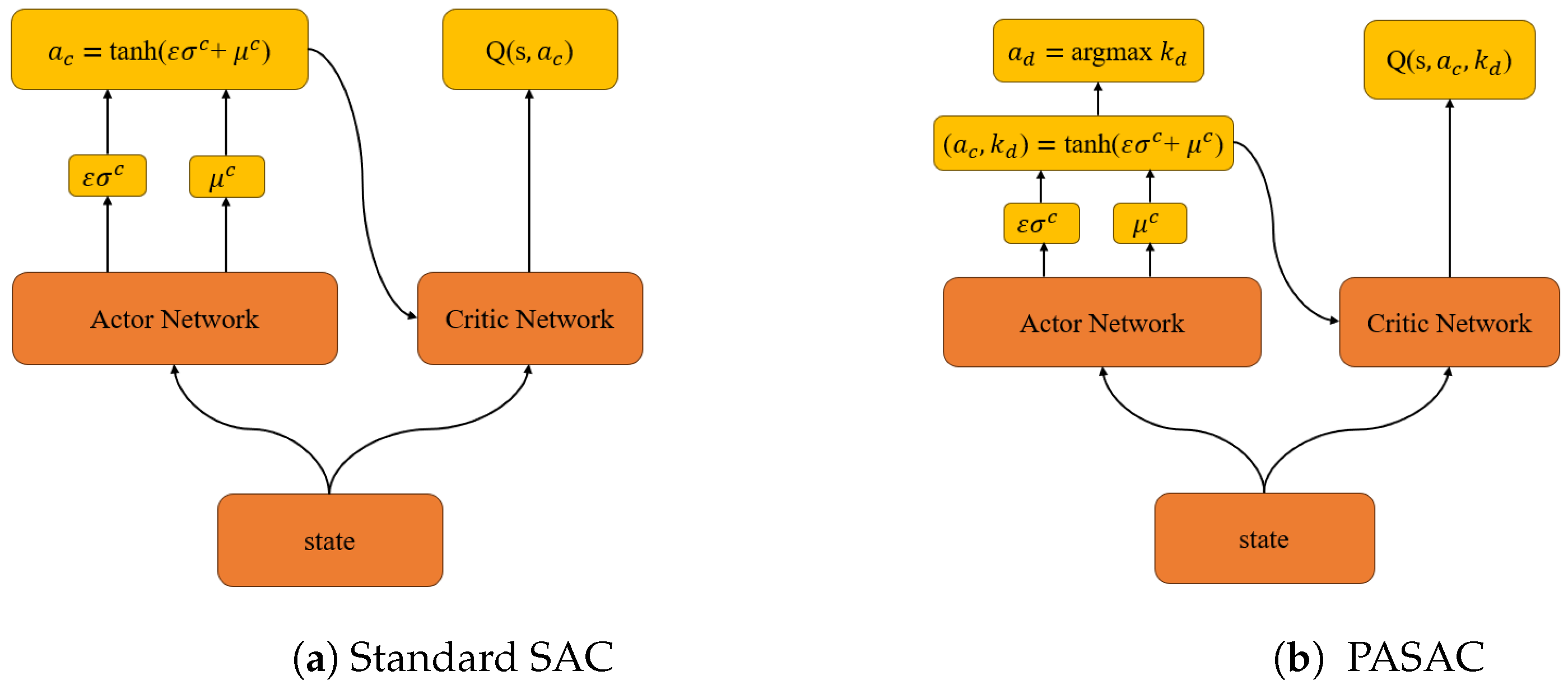
2.3. Parameterized Soft Actor–Critic

In this context, we define a Markov decision process with a parameterized action space. The action space consists of a set of discrete actions, denoted as $A_d=a_1,a_2,......a_n$. Each discrete action $a\in A_d$ is associated with a corresponding set of continuous parameters, represented as $a_1^{p_1},a_2^{p_2},......a_n^{p_n}$. In our environment, the actor network outputs m continuous parameters to form continuous actions and selects $n-m$ continuous parameters as weights for the discrete actions ($m<n$). The discrete action is determined by choosing the action with the maximum weight among the $n-m$ continuous parameters, expressed as $a_d=max(a_{m+1},a_{m+2},......a_n)$. The role of the actor network is to simultaneously decide which discrete action to execute and how to parameterize that action. Here, we adopt an approach similar to Delalleau 2019 [31], but unlike the former, our discrete actions are deterministic rather than stochastic.

The PASAC algorithm is similar to the algorithm proposed by Peter Stone in 2016 [18], as illustrated below: The actor neural network can directly output continuous actions, and for discrete actions, it outputs the action with the maximum weight, where the weights are normalized within the range [0, 1]. The training process of the PASAC algorithm is shown in Algorithm 1.

Algorithm 1 PASAC Algorithm Training Process.

Input:  $\theta$, $\psi$, $\widehat{\psi }$, $\varphi$               $\widehat{\psi }$←$\psi$, D←∅         For each iteration do             For each environment step do                $({\mathbf{a}}_c,{\mathbf{k}}_d)\sim {\pi }_{\varphi }\left({\mathbf{a}}_t\right|{\mathbf{s}}_t)$                ${\mathbf{a}}_d\sim argmax{\mathbf{k}}_d$                ${\mathbf{s}}_{t+1}\sim p\left({\mathbf{s}}_{t+1}\right|{\mathbf{s}}_t,{\mathbf{a}}_t)$                $D\leftarrow D\bigcup \left\{({\mathbf{s}}_t,{\mathbf{a}}_t,\mathbf{r}({\mathbf{s}}_t,{\mathbf{a}}_t),{\mathbf{s}}_{t+1})\right\}$             End for             For each gradient step do                ${\theta }_i\leftarrow {\theta }_i-{\lambda }_Q{\widehat{▽}}_{{\theta }_i}{J}_Q\left({\theta }_i\right)$ for $i\in \{1,2\}$                $\varphi \leftarrow \varphi -{\lambda }_{\pi }{\widehat{▽}}_{\varphi }{J}_{\pi }\left(\varphi \right)$                $\psi \leftarrow \psi -{\lambda }_V{\widehat{▽}}_{\psi }{J}_V\left(\psi \right)$                $\widehat{{\psi }_i}\leftarrow \tau {\psi }_i+(1-\tau ){\widehat{\psi }}_i$             End for         End for Output$\theta$, $\psi$, $\varphi$

In order to gain a comprehensive understanding of the decision-making process of the PASAC algorithm, we provide a detailed explanation of its neural network framework. Refer to Figure 1 for an illustration. In the structure diagram, the agent has two branches for handling actions—one for processing continuous actions and another for processing discrete actions. The outputs of these two branches are integrated into the final action decision, enabling the agent to learn and execute tasks in a mixed-action space.

3. PASAC for Lane Changing

In this section, we utilize the open-source simulator SUMO [32]. This integrated framework is employed to construct the RL environment, governing the behavior of autonomous vehicles. We present a model for autonomous lane changing based on reinforcement learning. By explicitly modeling states, actions, and rewards, the objective is to realize intelligent lane-change decisions for vehicles navigating through intricate traffic scenarios.

3.1. Scenario Settings

In the conducted experiments detailed in this paper, we utilized a straight roadway with a length of 1000 m and two lanes. The lane change scenario in SUMO is shown in Figure 2, the red car represents the ego vehicle, while the green cars represent the surrounding vehicles.

3.2. State

At time t, the distance between the ego vehicle and the preceding vehicle $d_t^p$, the distance between the ego vehicle and the following vehicle $d_t^f$, the distance from the ego vehicle to the preceding vehicle in the target lane $d_t^{targe{t}_p}$, the distance from the ego vehicle to the following vehicle in the target lane $d_t^{targe{t}_f}$, ego vehicle’s speed $v_{ego}$, ego vehicle’s acceleration $a_t^{ego}$, the speeds of the preceding car and following car $v_t^p,v_t^f$, as well as the speeds of the preceding and trailing cars in the target lane $v_t^{targe{t}_p},v_t^{targe{t}_f}$.

$$s=(d_t^p,d_t^f,d_t^{targe{t}_p},d_t^{targe{t}_f},v_t^{targe{t}_p},v_t^{targe{t}_f},v_t^{ego},a_t^{ego},v_t^p,v_t^f)\in S$$

(11)

3.3. Action

In this context, we define the action space as

$$a=\left\{a_t^{ego},0,1\right\}\in A,$$

(12)

In Equation (12), the symbol ‘0’ signifies the choice to postpone the lane change, indicating the intent to maintain the current position within the ego lane. Conversely, the symbol ‘1’ represents an immediate decision to execute the lane change, manifesting the intention to promptly transition to the target lane. These symbols denote discrete actions. ‘$a_t^{ego}$’, on the other hand, is a continuous action representing the acceleration of the ego vehicle.

3.4. Reward

The reward function is crafted with the objective of motivating positive behaviors and discouraging undesirable actions within the decision-making process of autonomous vehicles. In this paper, distinct rewards are allocated for tasks such as distance control, successful lane changes, adherence to speed limits, and collision avoidance. Drawing upon this concept, we formulated the following reward function.

$$R_{total}=R_{act}+R_{act1}+R_{act2}+R_{collision}$$

(13)

where $R_{total}$ is the total reward for the simulation scene. Where $R_{collision}$ is the penalty for vehicle collisions.

$$R_{act}=-{\omega }_0|y_{t-1}-y_t|$$

(14)

In Equation (14), $R_{act}$ is the penalty for frequent lane changes by vehicles, $w_0$ is the corresponding weight, and $y_t$ and $y_{t-1}$ represent the current and previous time step’s lateral positions of the vehicle. Note that when the distance to the preceding vehicle satisfies the ACC spacing, this reward penalty will not be computed, thus aligning with the MPC cost function.

Through a comprehensive analysis of the disparity between the actual speed and the desired speed of the ego vehicle, coupled with meticulous management of the spacing between the ego vehicle and its preceding and following counterparts, we skillfully crafted a longitudinal acceleration control strategy. The primary aim of this strategy is to mitigate the likelihood of collisions between vehicles, strategically initiating lane-change maneuvers during instances of reduced speed in the ego vehicle, thereby further optimizing the overall travel time. In consideration of passenger comfort, we implemented a penalty mechanism for changes in longitudinal acceleration, seeking to strike a harmonious balance between driving efficiency and the overall passenger experience. The specific reward function is delineated as follows:

$$R_{act1}=-{\omega }_1|d_t^p-d_{safe}|-{\omega }_2|d_t^f-d_{safe}|-{\omega }_3|v_{ego}-v_{safe}|$$

(15)

$$R_{act2}=-{\omega }_4\left|jerk\right|$$

(16)

In Equations (15) and (16), $w_1$, $w_2$, $w_3$, and $w_4$ denote the corresponding weights. Here, $d_{\mathit{safe}}$ represents the desired safe distance, $v_{\mathit{safe}}$ is the desired safe speed, and $jerk$ signifies the rate of change of acceleration for the ego vehicle.

In order to comprehensively present the key parameters involved in our analysis, we introduce a parameter table (

Table 1. Simulation parameters.

Parameters	Value	Weights	Value
$a_{min}$	−4.5 m/s2	$w_0$	3.13
$a_{max}$	2.6 m/s2	$w_1$	0.5
$v_{safe}$	13.89 m/s	$w_2$	0.4
$d_{safe}$	25 m	$w_3$	0.72
$R_{collision}$	−200	$w_4$	0.5

) at this point. It is worth noting that the weights were determined though manual turning.

4. Model Predictive Control Model

In MPC, the control inputs are determined by solving an optimization problem at each time step, taking into account the current state of the system and predicting its evolution over the horizon. This optimization process aims to minimize a predefined cost function, Here, we compare the costs for different lanes and initiate a lane change for the lane with the lowest cost. The lane change is instantaneous, wherein no lateral control is considered, the same as for DRL.

It is worth noting that we used YALMIP to handle optimization solutions. By leveraging the open-source YALMIP, we formulated and solved the MPC optimization problem. YALMIP can be installed in MATLAB, providing programmers with various shooting and optimization methods to address nonlinear optimization problems. In this section, the principles of the decision control for the self-driving vehicle under MPC are introduced. These include the state-space equations, cost function, constraints, future state estimation, and variable-spacing strategy.

4.1. State-Space Equations

The state-space equations for the MPC we implemented are as follows: It is worth noting that we simplified vehicles to a point mass, without considering the vehicle dynamics [33], as for DRL.

$$\begin{array}{cc}\hfill d_t^p& =s_p-s,\hfill \\ \hfill d_t^f& =s-s_f,\hfill \\ \hfill v_{ego}& =\dot{s},\hfill \\ \hfill ▵v_t^p& ={\dot{s}}_p-\dot{s}=v_p-v_{ego},\hfill \\ \hfill ▵v_t^f& =\dot{s}-{\dot{s}}_f=v_{ego}-v_f,\hfill \\ \hfill a_t^{ego}& ={\dot{v}}_{ego},\hfill \\ \hfill j_t^{ego}& ={\dot{a}}^{{ego}_t}\hfill \end{array}$$

(17)

$$x={\left[d_t^p,d_t^f,v_{ego},▵v_t^p,▵v_t^f,a_t^{ego},j_t^{ego}\right]}^T$$

(18)

$$u=a$$

(19)

$$x(k+1)=\mathbf{A}x\left(k\right)+\mathbf{B}u\left(k\right)$$

(20)

with

$$\mathbf{A}=\left[\begin{array}{ccccccc}1& 0& -T_s& T_s& 0& 0& 0\\ 0& 1& T_s& 0& -T_s& 0& 0\\ 0& 0& 1& 0& 0& T_s& 0\\ 0& 0& 0& 1& 0& 0& 0\\ 0& 0& 0& 0& 1& 0& 0\\ 0& 0& 0& 0& 0& 0& 0\\ 0& 0& 0& 0& 0& -1/T_s& 0\end{array}\right],\mathbf{B}=\left[\begin{array}{c}0\\ 0\\ 0\\ 0\\ 0\\ 1\\ 1/T_s\end{array}\right],$$

(21)

In Formula, s represents the longitudinal coordinate of the vehicle. x is utilized as the input, where $d_t^p$ and $d_t^f$ denote the distances to the preceding and following vehicles, respectively. The variables $▵v_t^p$ and $▵v_t^f$ represent the ego vehicle velocity differences with the preceding and following vehicles, while $v_{ego}$, $a_t^{ego}$, and $j_t^{ego}$ denote the velocity, acceleration, and jerk of the vehicle, respectively. u represents the control variable, where $T_s$ is the time interval, with $T_s$ set to 0.1 s.

4.2. Cost Function

$$J={\omega }_1|d_t^p-d_{safe}|+{\omega }_2|d_t^f-d_{safe}|+{\omega }_3|v_{ego}-v_{safe}|+{\omega }_4\left|jerk\right|$$

(22)

Formula (22) is consistent with the PASAC reward function. The primary objectives of the first and second terms are to ensure appropriate distances with the lead and following vehicles. The distance with the following vehicle is not penalized for the current lane, while it is penalized for the target lane. The third term aims to maintain a safe ego speed. The fourth term is designed to enhance driving comfort by penalizing jerk. The MPC cost does not include a penalty for frequent lane changes.

4.3. Future State Estimation

In the prediction horizon of MPC, scholars like Paolo Falcone fixed the values of slip and friction coefficients within the predictive time horizon, ensuring they remained constant and equal to the estimated values at the current moment [34]. Similarly, in this paper, we chose N = 5 as the prediction horizon and utilized the same velocity of the leading vehicle at the current time step during the prediction horizon.

4.4. TLACC (Two-Lane Adaptive Cruise Control)

TLACC is a decision and control algorithm based on MPC (Algorithm 2). Where $J_c$ and J denote the future driving costs for the current lane and the target lane, respectively. $l_{sw}$ is the lane change signal, where 0 indicates staying in the current lane, and 1 indicates a change to the target lane. $J_{th}$ is the threshold value for the future driving cost on the current lane that must be satisfied for a lane change, with $J_{th}$ set to 0.8. $u_d^c$ is the desired control input, and $u_d$ and $u_{target}$ are the expected control inputs for driving on the current lane and the target lane, respectively. $k_p$ is the extra weight for the future driving cost during a lane change, with $k_p$ set to 0.1. The extra weight prevents frequent lane changes.

Algorithm 2 TLACC Algorithm Process.

Input:  $d_t^p,d_t^f,▵v_t^p,▵v_t^f,a_t^{ego},j_t^{ego},l_t^c,v_{ego}$ Output:  $u_d,l_{sw}$         While TLACC engaged do             $(J_c,u_d^c)\leftarrow MPC(d_t^p,d_t^f,▵v_t^p,▵v_t^f,a_t^{ego},j_t^{ego},l_t^c,v_{ego})$             If $J_c\le J_{th}$ Then                    Return  $l_{sw}\leftarrow 0,u_d\leftarrow u_d^c$             else                   $(J,u_{target})\leftarrow MPC(d_{target}^p,d_{target}^f,▵v_{target}^p,▵v_{target}^f,a_t^{ego},j_t^{ego},l_{target},v_{ego})$                    If  $(1+k_p)J\le J_c$ Then                           Return  $l_{sw}\leftarrow 1,u_d\leftarrow u_{target}$                    else                           Return  $l_{sw}\leftarrow 0,u_d\leftarrow u_d^c$                    End             End         End

5. Comparison Results of DRL and MPC

Under the same conditions of relevant cost functions, input states, and traffic flow, this section presents the test results of the DRL and MPC controllers.

5.1. DRL Training

For the training of the reinforcement learning model, we chose total simulation timesteps of 300,000, with each timestep set to 0.1 s. The training was conducted on a computer equipped with an 8-core (16-thread) AMD processor and an NVIDIA GeForce RTX 3050 Ti GPU, and the training process took approximately 3 h. It is noteworthy that, before the start of each episode, there was a 50-m buffer for the initialization of main-road traffic.

In our study, to achieve effective training of the reinforcement learning model, we meticulously selected and configured a set of crucial hyperparameters. The choice of these hyperparameters directly impacted the model’s performance and the stability of the training process. In

Table 2. PASAC Hyperparameters.

Hyperparameters	Value	Hyperparameters	Value
Discount factor	0.99	Tau	0.005
Alpha	0.05	Learning starts	500
Actor learning rate	0.0001	Mini-batch size	128
Critic learning rate	0.001	Buffer size	10,000

, we provide a detailed list of the hyperparameters utilized during training, along with their corresponding values.

5.2. DRL Testing

The trained policy underwent additional testing with an extended 350,000 simulation time steps, representing 500 episodes. In order to better assess the performance of the model, we selected a typical initial condition where the leading vehicle’s initial velocity was set to 12.89 m/s, and the ego vehicle’s initial velocity was set to 13.89 m/s. The traffic flow density was 0.11 vehicles/second, for two lanes.

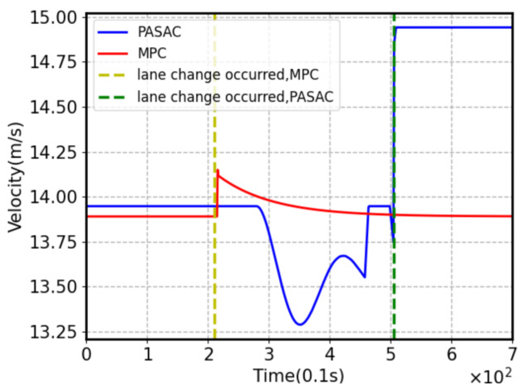
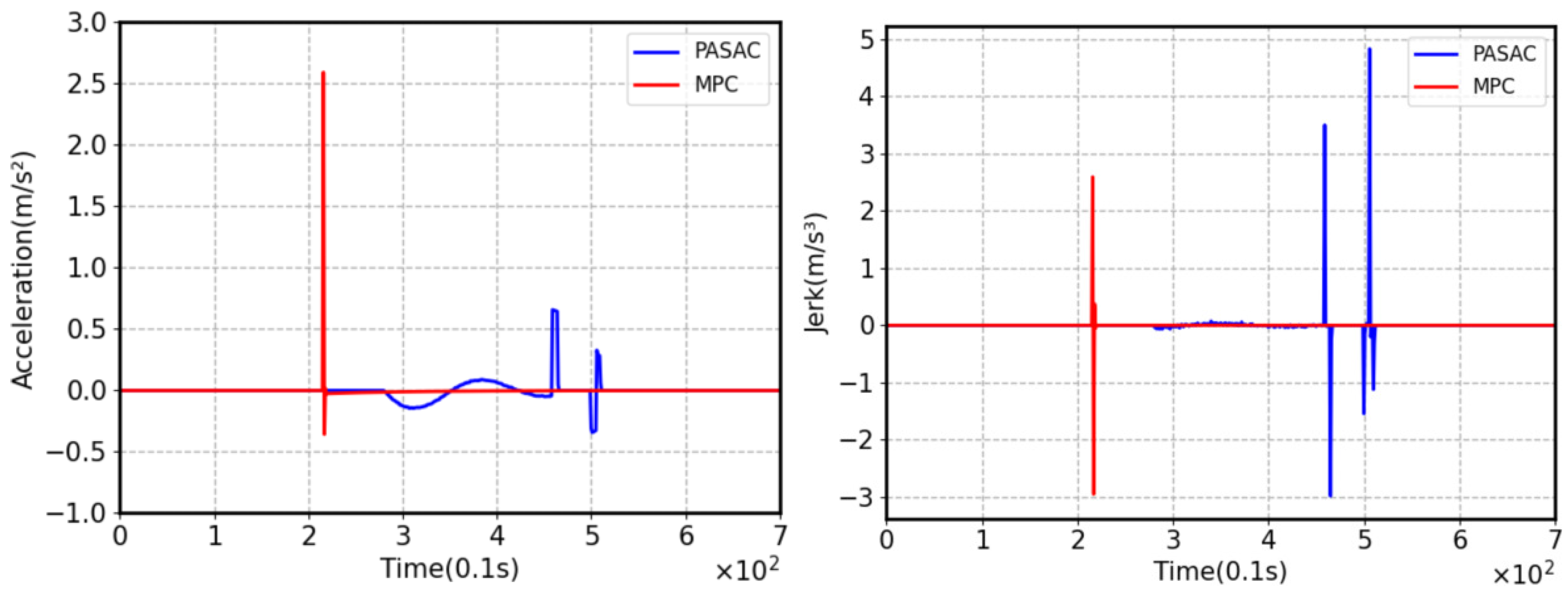
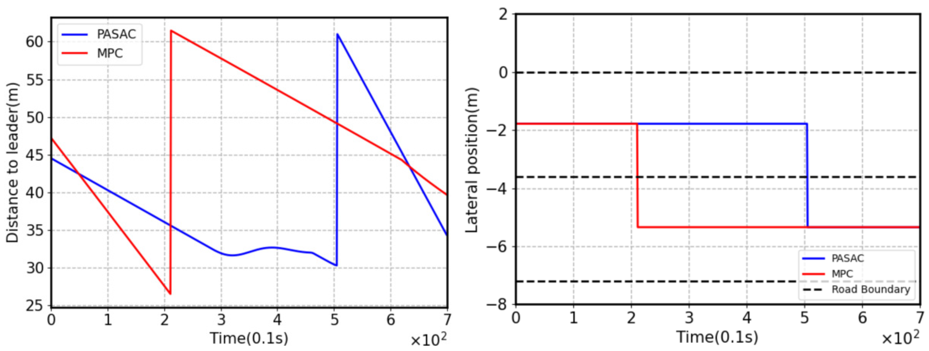
5.3. Comparison and Analysis

In the following sections, we compare the performance of MPC and RL in executing lane-change tasks for autonomous vehicles.

In Figure 3, the solid line represents the training curve of PASAC, and it can be observed that it approached convergence around 150,000 steps. The dashed line represents the total cost of MPC averaged over 5 episodes. The performance comparison results between PASAC and MPC are shown in

Table 3. Comparison of results from 100 episodes of testing.

	Collision	Average Speed (m/s)	Lane Change Times	Reward (Cost)	Reward (Cost) Difference
PASAC	0%	14.34	34	−27.73	27.90%
MPC	0%	13.95	25	−38.46	0%

. The average speed and cost for PASAC were superior to MPC. This implies that PASAC achieved better speed and time performance. Additionally, PASAC tended to execute more lane changes compared to MPC.

In Figure 4, the red solid line represents the self-driving vehicle controlled by the MPC method, while the deep blue solid line represents the vehicle controlled by the reinforcement learning algorithm PASAC. With PASAC, the vehicle decelerated suddenly and then accelerated, while with MPC, it accelerated first and then decelerated. The green and yellow dashed lines respectively represent lane changes by the self-driving vehicle under PASAC and MPC.

It can be observed that the lane changes under PASAC and MPC occurred at different times (MPC occurred around 22 s, while PASAC occurred around 51 s). This was because, for PASAC and MPC, the surrounding vehicles were in different states before the sudden lane change occurred. The self-driving vehicle under PASAC changed lanes immediately after a sudden deceleration, then accelerated to maintain a higher speed. On the other hand, the self-driving vehicle under MPC changed lanes after a sudden acceleration, maintaining a stable speed.

In the simulation results depicted in Figure 5, the acceleration and jerk of both MPC and PASAC demonstrate smooth motion characteristics, avoiding abrupt accelerations and vibrations, significantly enhancing the comfort of the driver. Figure 6 depicts the lateral position and distance to the leading vehicle in the simulations of PASAC and MPC for the ego vehicle.

Figure 6 illustrates the distance from the ego vehicle to the leading vehicle, with a set safety following distance of 25 m. To optimize the safety, both MPC and PASAC choose to initiate lane changes before reaching the 25 m distance to the leading vehicle. Note that there was a sudden change in the distance between the ego vehicle and the leading vehicle, indicating a successful lane change and a subsequent alteration in the state of the leading vehicle.

The lateral position of the autonomous vehicle on the road is shown in Figure 6, with dashed lines representing the road boundaries and solid lines distinctly outlining the precise location of the vehicle along the center line of the road. Through the visual contrast between the dashed and solid lines, we can clearly observe where the ego vehicle initiated lane changes.

5.4. Generalization Analysis

The complexity and dynamism of the environment can lead to a sub-optimal performance of the policy obtained during the training phase when applied to unseen settings. To thoroughly assess the algorithm’s performance, we conducted a series of tests encompassing 100 episodes, including traffic densities of 0.05 and 0.20.

Table 4. The generalization results across different traffic densities for 100 episodes.

		Collision	Average Speed (m/s)	Lane Change Times	Reward (Cost)	Reward (Cost) Difference
Traffic flow density $\varphi =0.05$ (veh/s )	PASAC	0%	14.40	24	−25.74	29.78%
	MPC	0%	13.97	19	−36.66	0%
Traffic flow density $\varphi =0.20$ (veh/s)	PASAC	0.2%	14.25	46	−27.53	30.63%
	MPC	0%	13.92	33	−39.69	0%

The traffic flow density is $\varphi$ = 0.11 vehicles/second (veh/s) during training.

presents the performance metrics, including the collision rate, average speed, and cost, across the various testing stages. Our findings indicate that, following testing in multiple traffic densities, the algorithm exhibited relatively stable performance in new environments.

6. Conclusions

In this study, we used a hybrid-action reinforcement learning algorithm, PASAC, and compared it with MPC for decision and control problems of autonomous vehicles during the lane-change process. Both MPC and PASAC achieved a collision rate of 0%. They shared the same control update frequency and were capable of handling hybrid-action space problems. We maintained identical testing conditions for PASAC and MPC, including traffic density and traffic scenarios. The results indicated that, in the absence of modeling errors, PASAC outperformed MPC in terms of the value function. Nevertheless, the PASAC algorithm still encountered collisions in scenarios with higher traffic flow, due to inadequate machine learning generalization. One of the challenges lies in the lack of theoretical analysis of the relationship between neural networks and optimal control, which could be a crucial area for future research.In the future, we also will consider more complex conditions, such as harsh weather conditions and unexpected road incidents.

References

1. Urmson, C.; Anhalt, J.; Bagnell, D.; Baker, C.; Bittner, R.; Clark, M.N.; Dolan, J.; Duggins, D.; Galatali, T.; Geyer, C.; et al. Autonomous driving in urban environments: Boss and the urban challenge. J. Field Robot. 2008, 25, 425–466. [Google Scholar] [CrossRef]
2. Hetrick, S. Examination of Driver Lane Change Behavior and the Potential Effectiveness of Warning Onset Rules for Lane Change or “Side” Crash Avoidance Systems. Master’s Dissertation, Virginia Polytechnic Institute & State University, Blacksburg, VA, USA, 1997. [Google Scholar]
3. Nilsson, J.; Brännström, M.; Coelingh, E.; Fredriksson, J. Lane change maneuvers for automated vehicles. IEEE Trans. Intell. Transp. Syst. 2016, 18, 1087–1096. [Google Scholar] [CrossRef]
4. Li, S.; Li, K.; Rajamani, R.; Wang, J. Model predictive multi-objective vehicular adaptive cruise control. IEEE Trans. Control. Syst. Technol. 2010, 19, 556–566. [Google Scholar] [CrossRef]
5. Ji, J.; Khajepour, A.; Melek, W.W.; Huang, Y. Path Planning and Tracking for Vehicle Collision Avoidance Based on Model Predictive Control With Multiconstraints. IEEE Trans. Veh. Technol. 2017, 66, 952–964. [Google Scholar] [CrossRef]
6. Raffo, G.V.; Gomes, G.K.; Normey-Rico, J.E.; Kelber, C.R.; Becker, L.B. A Predictive Controller for Autonomous Vehicle Path Tracking. IEEE Trans. Intell. Transp. Syst. 2009, 10, 92–102. [Google Scholar] [CrossRef]
7. Xu, Y.; Chen, B.Y.; Shan, X.; Jia, W.H.; Lu, Z.F.; Xu, G. Model predictive control for lane keeping system in autonomous vehicle. In Proceedings of the 2017 7th International Conference on Power Electronics Systems and Applications-Smart Mobility, Power Transfer & Security (PESA), Hong Kong, China, 12–14 December 2017; IEEE: Piscataway, NJ, USA, 2017; pp. 1–5. [Google Scholar]
8. Samuel, M.; Mohamad, M.; Hussein, M.; Saad, S.M. Lane keeping maneuvers using proportional integral derivative (PID) and model predictive control (MPC). J. Robot. Control (JRC). 2021, 2, 78–82. [Google Scholar] [CrossRef]
9. Hang, P.; Lv, C.; Xing, Y.; Huang, C.; Hu, Z. Human-Like Decision Making for Autonomous Driving: A Noncooperative Game Theoretic Approach. IEEE Trans. Intell. Transp. Syst. 2021, 22, 2076–2087. [Google Scholar] [CrossRef]
10. Hang, P.; Lv, C.; Huang, C.; Cai, J.; Hu, Z.; Xing, Y. An Integrated Framework of Decision Making and Motion Planning for Autonomous Vehicles Considering Social Behaviors. IEEE Trans. Veh. Technol. 2020, 69, 14458–14469. [Google Scholar] [CrossRef]
11. Mnih, V.; Kavukcuoglu, K.; Silver, D.; Rusu, A.A.; Veness, J.; Bellemare, M.G.; Graves, A.; Riedmiller, M.; Fidjel, A.K.; Ostrovski, G.; et al. Human-level control through deep reinforcement learning. Nature 2015, 518, 529–533. [Google Scholar] [CrossRef] [PubMed]
12. Van Hasselt, H.; Guez, A.; Silver, D. Deep reinforcement learning with double Q-learning. In Proceedings of the Thirtieth AAAI Conference on Artificial Intelligence, Phoenix, AZ, USA, 12–17 February 2016; Volume 30, pp. 2094–2100. [Google Scholar]
13. Hessel, M.; Modayil, J.; Van Hasselt, H.; Schaul, T.; Ostrovski, G.; Dabney, W.; Horgan, D.; Piot, B.; Azar, M.; Silver, D. Rainbow: Combining improvements in deep reinforcement learning. In Proceedings of the Thirty-Second AAAI Conference on Artificial Intelligence, New Orleans, LA, USA, 2–7 February 2018; Volume 32, pp. 3215–3222. [Google Scholar]
14. Lillicrap, T.P.; Hunt, J.J.; Pritzel, A.; Heess, N.; Erez, T.; Tassa, Y.; Silver, D.; Wierstra, D. Continuous control with deep reinforcement learning. In Proceedings of the International Conference on Learning Representations, San Juan, Puerto Rico, 2–4 May 2016. [Google Scholar]
15. Fujimoto, S.; Hoof, H.; Meger, D. Addressing function approximation error in actor-critic methods. In Proceedings of the International Conference on Machine Learning, Stockholm, Sweden, 10–15 July 2018; Volume 80, pp. 1587–1596. [Google Scholar]
16. Haarnoja, T.; Zhou, A.; Abbeel, P.; Levine, S. Soft actor-critic: Off-policy maximum entropy deep reinforcement learning with a stochastic actor. In Proceedings of the International Conference on Machine Learning, Stockholm, Sweden, 10–15 July 2018; Volume 80, pp. 1861–1870. [Google Scholar]
17. Neunert, M.; Abdolmaleki, A.; Wulfmeier, M.; Lampe, T.; Springenberg, T.; Hafner, R.; Romano, F.; Buchli, J.; Heess, N.; Riedmiller, M. Continuous-discrete reinforcement learning for hybrid control in robotics. In Proceedings of the Conference on Robot Learning, Osaka, Japan, 30 October–1 November 2019; pp. 735–751. [Google Scholar]
18. Hausknecht, M.; Stone, P. Deep reinforcement learning in parameterized action space. In Proceedings of the International Conference on Learning Representations, San Juan, Puerto Rico, 2–4 May 2016. [Google Scholar]
19. Xiong, J.; Wang, Q.; Yang, Z.; Sun, P.; Han, L.; Zheng, Y.; Fu, H.; Zhang, T.; Liu, J.; Liu, H. Parametrized deep Q-networks learning: Reinforcement learning with discrete-continuous hybrid action space. arXiv 2018, arXiv:1810.06394. [Google Scholar]
20. Bester, C.J.; James, S.D.; Konidaris, G.D. Multi-pass Q-networks for deep reinforcement learning with parameterised action spaces. arXiv 2019, arXiv:1905.04388. [Google Scholar]
21. Li, B.; Tang, H.; Zheng, Y.; Jianye, H.A.O.; Li, P.; Wang, Z.; Meng, Z.; Wang, L.I. HyAR: Addressing Discrete-Continuous Action Reinforcement Learning via Hybrid Action Representation. In Proceedings of the International Conference on Learning Representations, Virtual, 25–29 April 2022. [Google Scholar]
22. Mukadam, M.; Cosgun, A.; Nakhaei, A.; Fujimura, K. Tactical decision making for lane changing with deep reinforcement learning. In Proceedings of the 6th International Conference on Learning Representations, Vancouver, BC, Canada, 30 April–3 May 2018. [Google Scholar]
23. Wang, P.; Chan, C.Y.; de La Fortelle, A. A reinforcement learning based approach for automated lane change maneuvers. In IEEE Intelligent Vehicles Symposium; IEEE: Piscataway, NJ, USA, 2018; pp. 1379–1384. [Google Scholar]
24. Alizadeh, A.; Moghadam, M.; Bicer, Y.; Ure, N.K.; Yavas, U.; Kurtulus, C. Automated lane change decision making using deep reinforcement learning in dynamic and uncertain highway environment. In Proceedings of the IEEE Intelligent Transportation Systems Conference, Auckland, New Zealand, 27–30 October 2019; pp. 1399–1404. [Google Scholar]
25. Saxena, D.M.; Bae, S.; Nakhaei, A.; Fujimura, K.; Likhachev, M. Driving in dense traffic with model-free reinforcement learning. In Proceedings of the IEEE International Conference on Robotics and Automation, Paris, France, 31 May–31 August 2020; pp. 5385–5392. [Google Scholar]
26. Wang, G.; Hu, J.; Li, Z.; Li, L. Harmonious lane changing via deep reinforcement learning. IEEE Trans. Intell. Transp. Syst. 2021, 23, 4642–4650. [Google Scholar] [CrossRef]
27. Guo, Q.; Angah, O.; Liu, Z.; Ban, X.J. Hybrid deep reinforcement learning based eco-driving for low-level connected and automated vehicles along signalized corridors. Transp. Res. Part C Emerg. Technol. 2021, 124, 102980. [Google Scholar] [CrossRef]
28. Vajedi, M.; Azad, N.L. Ecological adaptive cruise controller for plug in hybrid electric vehicles using nonlinear model predictive control. IEEE Trans. Intell. Transp. Syst. 2016, 17, 113–122. [Google Scholar] [CrossRef]
29. Lee, J.; Balakrishnan, A.; Gaurav, A.; Czarnecki, K.; Sedwards, S. Wisemove: A framework to investigate safe deep reinforcement learning for autonomous driving. In Proceedings of the Quantitative Evaluation of Systems: 16th International Conference, QEST 2019, Glasgow, UK, 10–12 September 2019; pp. 350–354. [Google Scholar]
30. Sutton, R.S.; Barto, A.G. Reinforcement learning. J. Cogn. Neurosci. 1999, 11, 126–134. [Google Scholar]
31. Delalleau, O.; Peter, M.; Alonso, E.; Logut, A. Discrete and continuous action representation for practical RL in video games. arXiv 2019, arXiv:1912.11077. [Google Scholar]
32. Krajzewicz, D.; Erdmann, J.; Behrisch, M.; Bieker, L. Recent development and applications of SUMO-Simulation of Urban MObility. Int. J. Adv. Syst. Meas. 2012, 5, 128–138. [Google Scholar]
33. Wang, Z.; Cook, A.; Shao, Y.; Xu, G.; Chen, J.M. Cooperative merging speed planning: A vehicle-dynamics-free method. In Proceedings of the 2023 IEEE Intelligent Vehicles Symposium (IV), Anchorage, AK, USA, 4–7 June 2023; IEEE: Piscataway, NJ, USA, 2023; pp. 1–8. [Google Scholar]
34. Falcone, P.; Borrelli, F.; Asgari, J.; Tseng, H.E.; Hrovat, D. Predictive active steering control for autonomous vehicle systems. IEEE Trans. Control Syst. Technol. 2007, 15, 566–580. [Google Scholar] [CrossRef]
Figure 1. (a) The framework on the left is the standard SAC architecture designed for continuous operation. The actor outputs mean and standard deviation vectors μ and σ , which are utilized for injecting standard normal noise ϵ and applying the tanh nonlinearity (to keep the actions within a bounded range). The critic estimates the corresponding Q value based on the state and the actor’s action a c . (b) On the right, we use the parameterized SAC structure. including the mean μ and the variance σ for the continuous components. It outputs continuous actions a c and k d . The largest k d among continuous actions is selected for the discrete action. The critic network still takes the state s, continuous actions a c and k d as inputs.
Machines 12 00213 g001
Figure 2. Lane change scenario in SUMO.
Machines 12 00213 g002
Figure 3. The reward (cost) between MPC and PASAC.
Machines 12 00213 g003
Figure 4. Lane change in the simulation.
Machines 12 00213 g004
Figure 5. Acceleration and jerk during the simulation.
Machines 12 00213 g005
Figure 6. Distance to the leader and lateral position during the simulation.
Machines 12 00213 g006