Article

Joint-Module Health Status Recognition for an Unmanned Platform: A Time–Frequency Representation and Extraction Network-Based Approach

1
School of Mechanical Engineering, Nanjing University of Science and Technology, Nanjing 210094, China
2
Southwest Automation Research Institute, Mianyang 621000, China
*
Author to whom correspondence should be addressed.
Machines 2024, 12(1), 79; https://doi.org/10.3390/machines12010079
Submission received: 11 December 2023 / Revised: 11 January 2024 / Accepted: 12 January 2024 / Published: 20 January 2024
(This article belongs to the Section Robotics, Mechatronics and Intelligent Machines)

Abstract

:
Due to the complex structure of the joint module and harsh working conditions of unmanned platforms, the fault information is often overwhelmed by noise. Moreover, traditional mechanical health state recognition methods usually require a large amount of labeled data in advance, which is difficult to obtain for specific fault data in engineering applications. This limited amount of fault data restricts the diagnostic performance. Additionally, the characteristics of convolutional neural networks (CNNs) limit their ability to capture the relative positional information of fault features. In order to obtain more comprehensive fault information, this paper proposes an intelligent health state recognition method for unmanned platform joint modules based on feature modal decomposition (FMD) and the enhanced capsule network. Firstly, the collected vibration signals are decomposed into a series of feature modal components using FMD. Then, time–frequency maps containing significant fault features are generated based on the continuous wavelet transform (CWT). Finally, a multi-scale feature enhancement (MLFE) module and an efficient channel attention (ECA) module are proposed to enhance the feature extraction capability of the capsule network, extracting more comprehensive global and local feature information from the time–frequency maps to achieve the intelligent state recognition of joint modules. This approach enhances fault features while reducing the impact of redundant features, significantly improving the feature extraction capability without increasing the model’s computational complexity. The effectiveness and superiority of the proposed method are validated through experiments on an unmanned platform joint-module testbed. An ablation experiment demonstrates the effectiveness of the MLFE and ECA modules, and a comparison with other advanced network models proves the superiority of the proposed method for health status recognition.

1. Introduction

Unmanned platforms refer to robots that perform unmanned operations through remote monitoring. As an emerging intelligent equipment, unmanned platforms have a wide range of applications in military, medical, energy, and other fields [1,2]. The joint module of unmanned platforms, as a key transmission mechanism, integrates a large number of components, including permanent magnet synchronous motors, planetary gear reducers, encoders, etc. [3,4], within a limited space. Considering the harsh working environment and the complexity of its structure, the mechanical components of unmanned platforms inevitably experience various faults, leading to significant economic losses and even endangering one’s safety. In practical situations, when mechanical components, such as bearings and gears, of the joint module fail, the collected vibration signals are inevitably contaminated by strong noise, making it difficult to effectively identify the fault types of the unmanned platform joint module [5]. Therefore, researching the efficient feature extraction and health status recognition of unmanned platform joint modules using vibration signals has significant engineering application value.
To date, non-stationary signal processing algorithms have been widely applied in the field of mechanical equipment fault diagnosis, such as short-time Fourier transform (STFT) and wavelet transform. However, these time–frequency analysis methods require the selection of suitable window functions or wavelet bases [6,7]. To address this issue, a series of signal decomposition methods based on empirical mode decomposition (EMD) [8,9] have been proposed and widely extended, such as variational mode decomposition [10], local mean decomposition [11], symplectic geometric mode decomposition [12], and empirical mode decomposition with improved time scales [13]. These signal decomposition methods can adaptively decompose complex signals into a series of intrinsic mode function (IMF) components. However, these decomposition methods often suffer from mode mixing when dealing with noisy non-stationary signals, affecting the final decomposition results. To overcome the shortcomings of the existing signal decomposition algorithms and improve the fault diagnosis performance, inspired by the deconvolution theory, Miao et al. proposed a new non-stationary signal decomposition algorithm called feature mode decomposition (FMD) [14]. The FMD method establishes an adaptive finite impulse response (FIR) filter and uses the iterative updating of filter coefficients. During each iteration, the fault period of the measured signal is estimated based on the correlation coefficient (CC) to decompose the non-stationary signal into several modal components. The FMD method not only simultaneously considers the periodicity and impulsive nature of the signal, but also exhibits certain anti-interference capabilities against noise, resulting in a more thorough decomposition.
Although various non-stationary signals can provide distinct fault features, they heavily rely on the application of expert systems for health status recognition, which is clearly not intelligent enough for the big data era of Industry 4.0. Therefore, many scholars have combined signal processing algorithms with intelligent classifiers. The signal processing algorithms can provide richer and more accurate fault features for subsequent intelligent classifiers. For example, Li et al. first used parameter-optimized variational mode decomposition (VMD) for signal decomposition, combined with a sample entropy to extract fault feature vectors, and finally introduced a support vector machine (SVM) to perform the fault diagnosis of rolling bearings [15]. Zhang et al. used an improved EMD for signal decomposition, combined with signal complexity, to reconstruct effective intrinsic mode functions (EIMFs) [16]. They then extracted ten time-domain features of EIMFs as inputs to deep belief networks (DBNs) for the diagnosis of rotating machinery faults. In addition, Kim et al. proposed a fault diagnosis method for high-speed train rotational components using a VMD algorithm based on the multi-verse optimization to decompose and reconstruct vibration signals, followed by the feature extraction of the reconstructed signals and the use of adaptive mutation particle swarm optimization-random forest (AMPSO-RF) [17]. Tong et al. combined the second-generation wavelet packet transform and local feature scale decomposition to decompose the vibration signal into multiple IMFs and applied the extreme learning machine (ELM) to perform the fault diagnosis of rolling bearings [18]. Tu et al. used an EEMD to decompose the original signal to obtain several IMFs, then conducted an overall average check and optimization of each IMF to obtain multiple sets to characteristic the values, and finally input the characteristic values into a KELM to perform the fault diagnosis of an RV reducer [19]. However, the aforementioned classifiers (such as the SVM, DBN, RF, ELM, etc.) are only shallow machine learning models, and are ineffective and lack robustness in the face of strong noise and limited training samples in practical situations.
To overcome these challenges, intelligent diagnostic models based on deep learning have garnered increasing attention and achieved numerous results for fault diagnosis. Chen et al. combined the complementary set empirical mode decomposition and STFT to generate a time–frequency diagram of noise reduction signals, and then used a CNN to automatically extract fault information from the time–frequency diagram and realize the fault diagnosis of rolling bearings [20]. Likewise, Tran et al. presented a two-dimensional time–frequency representation of vibration signals based on the continuous wavelet transform (CWT), combined with a CNN for an intelligent diagnosis of induction motors [21]. Zaman et al. utilized the S-transform and Sobel filter to create scaleograms with higher time–frequency resolutions. Subsequently, these scaleograms were provided to the CNN for the classification of centrifugal pump health conditions [22]. Tang et al. used the synchronous compressed wavelet transform to transform the original signal into a two-dimensional image, and then used the CNN for fault feature extraction and classification, ultimately validating the effectiveness using the vibration signals of a hydraulic piston pump, sound signals, and pressure signals [23]. Huang et al. decomposed the original vibration signal into multi-scale vibration components using the wavelet packet decomposition, then used the CNN to extract fault features from the multi-scale vibration components for the fault diagnosis of a wind turbine gearbox [24]. Xiong et al. combined a complementary ensemble empirical mode decomposition with multidimensional non-dimensional indicators to extract complementary ensemble multi-dimensional indicators (CEMDIs) from vibration signals, which were then transformed into two-dimensional data as the input for the CNN to perform the fault diagnosis of rotating machinery [25]. Zhang et al. proposed an adaptive multi-dimensional variational mode decomposition to decompose an original signal and used a multi-scale CNN to extract the fault features from the denoised signal for the fault-type recognition of rolling bearings [26]. Kim et al. incorporated a health-adaptive time-scale representation (HTSR) into a CNN to extract richer fault information and perform the intelligent diagnosis of gearboxes [27]. Zhang et al. used compressive sensing to compress and reconstruct vibration signals, then combined transfer learning and the CNN for the fault sample recognition of wind turbine generators [28]. Gu et al. first decomposed the original signal using the VMD, then used the continuous wavelet transform to transform the IMF decomposition into a two-dimensional time–frequency image, which was trained using a CNN to perform the online fault diagnosis of rotating machinery [29]. Xie et al. first converted the time domain signal into the frequency domain signal by using the fractional Fourier transform, then converted the amplitude spectrum and phase spectrum into a gram angle field diagram, and finally used the CNN to extract the information of the angle field diagram to realize fault diagnosis of rolling bearings [30].
Although the aforementioned intelligent diagnosis models achieve certain effectiveness, they still have some drawbacks. On the one hand, the fault features extracted by existing CNN models are scalar, unable to capture the relative positional relationships between fault features, leading to the loss of fault-related information. On the other hand, existing CNN models are often composed of a large number of feature extraction modules, which, limited by this, often become stuck in local optimizations during the training process, and even lead to the degradation of the final recognition capability. Therefore, to address these challenges, this paper proposes a new method for the intelligent health status recognition of unmanned platform joint modules based on the FMD and enhanced capsule network. This method integrates a multi-scale feature enhancement module (MLFE module) and attention mechanism, constructing an intelligent health status recognition model based on the multi-scale feature enhancement module and efficient channel attention module for the enhanced capsule network. The capsule network [31] adopts feature vectors as the input to reduce the loss of fault feature information, while the MLFE module and attention mechanism enhance the model’s ability to extract fault features.
In summary, this paper proposes a novel approach for the intelligent health status recognition of joint modules in an unmanned platform based on time–frequency representation and enhanced capsule network. The method initially employs the FMD and CWT to extract time–frequency features from the vibration signals. Subsequently, these time–frequency representations are input into an improved capsule network for the fault diagnosis of joint modules in unmanned platforms. The main contributions of this paper are as follows:
(1)
Introduces a hybrid model based on the FMD, CWT, and capsule network for the fault diagnosis of joint modules in unmanned platforms.
(2)
Investigates the decomposition effectiveness of the FMD method on vibration signals. The signals processed by FMD are transformed into time–frequency representations using the CWT.
(3)
Proposes the multi-level feature enhancement (MLFE) module for integrating multi-scale features, and simultaneously utilizes the enhanced channel attention (ECA) module to adaptively extract crucial channel features to enhance the feature extraction capability of the capsule network.
The remaining sections of this study are as follows. Section 2 briefly outlines the basic theories of the continuous wavelet transform, FMD, and capsule network. In Section 3, the proposed MLFE module and efficient channel attention module, as well as the overall structure of the proposed method for health status recognition, are introduced. Section 4 describes the overall roadmap of the proposed intelligent health status recognition framework. Section 5 validates the effectiveness and robustness of the proposed method through the study and comparative analysis of the experimental platform for unmanned platform joint modules. Section 6 provides the conclusion of this work.

2. Basic Theory

2.1. Continuous Wavelet Transform

Studies show that one-dimensional time-domain signals are not the best method to reveal fault information, and the research also demonstrates that two-dimensional-type images can represent more complex distributions, thus providing a more distinct way to distinguish different fault distributions. Furthermore, CapsNet was initially proposed for 2D-image classification tasks, making it more suitable for processing 2D data. The CWT is a time–frequency transformation method that is very suitable for analyzing non-stationary signals, as it can accurately locate the frequency information corresponding to each moment [32]. Therefore, in order to improve the diagnostic performance, the CWT is used to extract deep time–frequency features from the original vibration signal as the input to the intelligent fault diagnosis model.
For a continuous time signal, f ( t ) , the definition of the continuous wavelet transform is:
W b ( a ) = ψ a , b ( t ) , x ( t ) = | a | 1 2 + f ( t ) ψ ( ( t b ) a ) d t
In Equation (1), a and b are the scale and translation factors of the wavelet function, respectively, determining the time–frequency window of the wavelet in the frequency and time domains, while ψ ( t ) represents the wavelet function being used.
The wavelet function is a function with local properties in the time–frequency domain. In this paper, we used the Morlet wavelet because of its concentrated frequency energy, narrow bandwidth, minimal frequency aliasing effects, time-domain symmetry, and linear phase characteristics, ensuring a distortion-free transformation.
Due to the discrete nature of the measured signal, for a discrete time series, f m , let t = m t , b = n t , where m , n = 0 , 1 , 2 , N 1 , N is the number of sampling points, and t is the sampling time interval. The continuous wavelet transform of the discrete time series, x m , is given by:
W n ( a j ) = m = 0 N 1 f m ψ [ ( m n ) Δ t a j ]
By changing the scale factor, a, and the translation factor, b, corresponding to the time indices j and n, a continuous wavelet transform coefficient matrix can be obtained, which reflects the variation of the amplitude of the continuous wavelet transform coefficients with time and scale.

2.2. Feature Mode Decomposition

Inspired by the deconvolution theory, the FMD method is a non-recursive decomposition method aimed at partitioning the original signal into different modes through the design of FIR filter banks. It mainly involves processes, such as an adaptive FIR filter design, filter updating, period estimation, and mode decomposition. Due to the strong dependence of the decomposition results on the filter coefficients, FMD is ultimately considered as a constrained problem solution, which can be expressed as:
arg max { C K M ( u k ) = n = 1 N ( m = 0 M u k ( n m T s ) ) 2 / ( n = 1 N u k ( n ) 2 ) M + 1 } s . t . u k ( n ) = l = 1 L f k ( l ) x ( n l + 1 )
where CK is the objective function, which can simultaneously evaluate the periodicity and impulsiveness of the signal. It is the n-th decomposition mode and K-th FIR filter with a length of L. M represents the input periodicity and shift order.
To solve the constrained problem in (3), we used the iterative eigenvalue decomposition algorithm. First, we rewrite the decomposition mode in matrix form:
u k = [ u k [ 1 ] u k [ N L + 1 ] ] = X f k = [ x ( 1 ) x ( L ) x ( N L + 1 ) x ( N ) ] [ f k ( 1 ) f k ( L ) ]
Then, the CK of the decomposition mode can be defined as:
C K M ( u k ) = u k H W M u k u k H u k
where the superscript H denotes the operation of the conjugate transpose, used for the intermediate variable of the weighted correlation matrix. Its expression is shown as:
W M = [ ( m = 0 M u k [ 1 m T s ] ) 2 0 0 0 ( m = 0 M u k [ 2 m T s ] ) 2 0 0 0 ( m = 0 M u k [ N L + 1 m T s ] ) 2 ] 1 n 1 N L + 1 u k [ n ] M 1
Substituting Equation (4) into Equation (5), we can obtain the following expression:
C K M ( u k ) = f k H X H W M X f k f k H X H X f k = f k H R X W X f k f k H R X X f k
where R X W X and R X X are the weighted correlation and correlation matrices, respectively. Mathematically, maximizing Equation (7) with respect to the filter coefficients is equivalent to solving for the eigenvector corresponding to the maximum eigenvalue, λ , in Equation (8):
R X W X f k = R X X f k λ
During the iteration process, the k-th filter coefficient was updated through the solution of Equation (8) to progressively approach the filter signal with the maximum CK.
Due to multi-modality, many modes can contain the same fault features. Therefore, FMD performs the mode selection by computing the Pearson CC to assess the similarity between two modes. The specific expression for CC is given by:
C C p q = n = 1 N ( u p ( n ) u ¯ p ) ( u q ( n ) u ¯ q ) n = 1 N ( u p ( n ) u ¯ p ) 2 n = 1 N ( u q ( n ) u ¯ q ) 2
where u ¯ p and u ¯ q are the mean values of modes u p and u q , respectively.
The overall implementation process of the FMD is as follows:
(1)
Load the original signal, x, and preset the parameters for the FMD, such as the decomposition mode, K; the filter length, L; and the maximum iteration count, I.
(2)
Initialize the FIR filter bank using M Hanning windows and start the iteration with i = 1. Typically, M is set to be within the range of 5–10.
(3)
Use u m i = x f m i to obtain the filtered signal or decomposed mode components, where m = 1, 2, … M; represents the convolution operation.
(4)
Update the filter coefficients and estimate the fault period based on the input original signal and decomposed mode components. Here, T m i is the time delay corresponding to the local maximum of the autocorrelation spectrum after the first zero crossing.
(5)
Check if the current iteration count has reached the maximum iteration count. If not, return to step (3); otherwise, proceed to step (6).
(6)
Compute the CC between two adjacent components and construct a correlation matrix. Select two adjacent mode components with the highest CC and calculate the CK values of the selected mode components based on the estimated fault period. Then, choose the mode component with the larger CK value as the FMD mode component and set M = M − 1.
(7)
Check if the current mode count has reached the preset mode count, K. If not, return to step (3); otherwise, stop the iteration and output the final decomposition results.

2.3. Capsule Network

A basic capsule network model is shown in Figure 1. Unlike a typical convolutional neural network, the capsule network performs a convolutional feature extraction, only in the initial part of the network. In the latter part, it replaces the original pooling and fully connected layers with a network-specific primary capsule layer and digit capsule layer. In this process, steps ➀ and ➁ are convolutional layers used to extract low-level convolutional features from the input image. The primary capsule layer is used to generate capsule activation vectors of specific dimensions. Step ➂ refers to the dynamic routing algorithm used to convert primary capsules into digit capsules. The digit capsule layer transforms the length of each capsule vector into the probability of each category appearing using a transformation matrix, and outputs the final classification result.
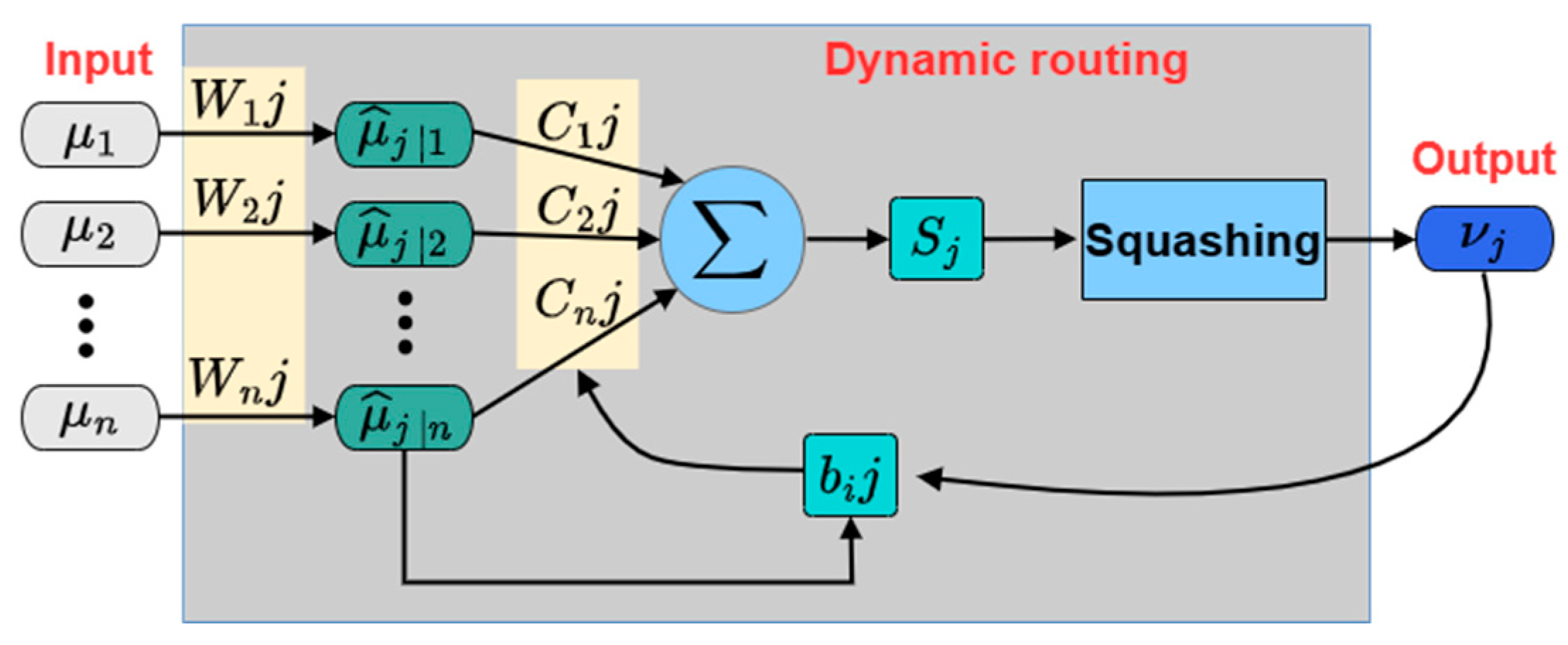
The capsule network differs from traditional artificial neurons in that it outputs a vector as a result, known as a capsule, which can effectively handle different types of visual stimuli and encode information, such as position, shape, and speed, reducing the loss of important information. When propagating from low-dimensional to high-dimensional capsules, the dynamic routing between the capsules allocates weights to the low-dimensional capsules, enhancing the feature recognition capability, as illustrated in Figure 2.
This process can be divided into the following steps:
(1)
The input is a set of lower-level capsules, where n represents the number of capsules and k represents the number of neurons in each capsule (vector length). Using a transformation matrix, W i j p × k , and p representing the number of neurons in the output capsule, the input u i k × i is transformed into the prediction vector:
μ j i = W i j μ i
where μ j | i p × 1 .
(2)
The weighted sum of all the obtained prediction vectors is calculated as:
s j = i C i j μ j i
where c i j is the coupling coefficient and j c i j = 1 .
(3)
The final vector, v j , is obtained through non-linear mapping by the squeezing function:
v j = s j 2 1 + s j 2 s j s j
where j represents the j-th output neuron. Essentially, the squeezing function is a normalization operation that causes the length of each vector fall between 0 and 1 (positively correlated with the original length), only changing the magnitude without affecting the direction; c i j and b i j are updated by the dynamic routing algorithm:
C i j = e b i j k e b i k
b i j = b i j + v j μ j i
In the forward propagation of the network, b i j is initialized as 0, C i j is initially calculated by Equation (14), and then v j is calculated based on the forward propagation. Equation (15) is used to update b i j and C i j , thereby further updating s j and v j .

2.4. Evaluation Metrics

During the process of evaluating a model, it is often necessary to use multiple different metrics for the assessment. Most evaluation metrics can only reflect certain aspects of the model’s performance. The incorrect usage of evaluation metrics can lead to incorrect conclusions and the failure to recognize issues with the model itself, making the correct and rational selection of evaluation metrics extremely important. For common binary classification problems, the classes are typically divided into positive and negative classes, with the positive class being the class of interest. Based on the correctness of the final prediction results, the predicted samples can be categorized into four types: the number of falsely predicted positive samples (False Positive, FP), the number of falsely predicted negative samples (False Negative, FN), the number of correctly predicted positive samples (True Positive, TP), and the number of correctly predicted negative samples (True Negative, TN). In practical fault classification problems, using only positive and negative classes to determine the state of a machine is clearly not detailed enough. It is necessary to differentiate between multiple fault types to thoroughly assess the mechanical fault state, thus requiring the use of evaluation metrics for multi-class problems. The evaluation metrics for multi-class problems have evolved from binary classifications, including metrics, such as accuracy, loss, and the confusion matrix.
In the binary classification, TP, FP, TN, and FN are scalar values, whereas in multi-class problems (taking n classes as an example), these values become n-dimensional vectors, with each dimension of the vector representing a specific value for a particular classification. A sample that is TP in one classification can become FP in another classification.
(1)
Accuracy represents the proportion of correct predictions to the total number, with a higher ratio indicating a better classification performance.
A c c u r a c y = ( T P + T N ) / ( T P + F P + T N + F N )
(2)
For multi-class classifications, the loss function commonly used is the cross-entropy loss function, where a smaller value indicates a better performance.
L o s s = 1 N i c = 1 M y i c log ( p i c )
(3)
The confusion matrix, also known as an error matrix, is a way to evaluate the performance of a classifier. It is an n × n matrix that describes the relationship between the true class attributes of the sample data and the predicted recognition classes, widely used for pattern recognition. Each row of the confusion matrix represents the true class attributes of the sample data, while each column represents the predicted recognition classes. It can be inferred that the higher the values on the diagonal of the confusion matrix, the better the classification recognition results.

3. Multi-Feature-Enhanced Efficient Channel Attention Fusion Capsule Network

3.1. Multi-Scale Feature Enhancement Module

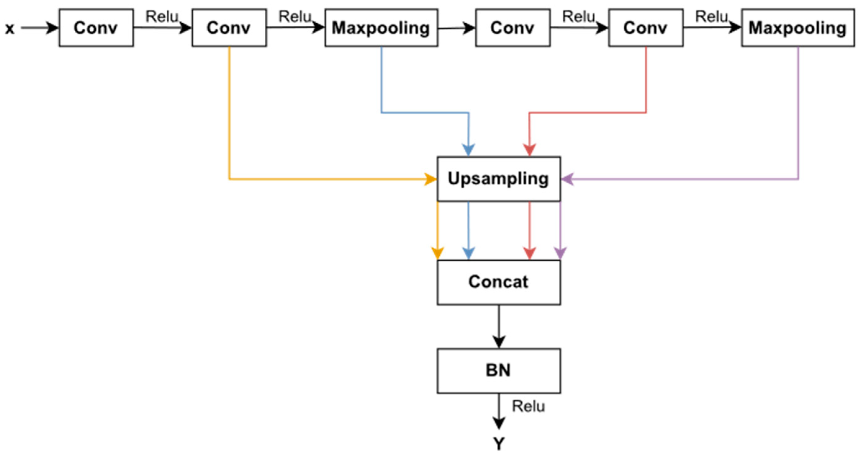
Traditional feedforward neural networks tend to produce increasingly localized feature maps as the network layers increase, leading to the loss of some crucial information from the original data in the intermediate layers of the neural network model. To address this deficiency, this paper proposed a method that could reduce the complexity of the neural network model while preventing the loss of intermediate layer information. This method is called the multi-scale feature enhancement (MLFE) module, as shown in Figure 3, where X and Y represent the input and output of the module, respectively. The arrows of different colors represent the flow of features of different scales within the structure. The input, X, undergoes a series of operations, including convolution, activation, pooling, upsampling, and concatenation, to obtain a vector, Y, with global features of the input, X. As shown in the figure, the initial structure of this module is based on the common standard structure for image classification, with an added auxiliary structure that allows the module to obtain features of different sizes during the feedforward process. Since features at each scale have different resolutions during the feedforward process, they are upsampled using a bilinear interpolation to achieve the same resolution. Ultimately, the feature maps from all scales are concatenated to form a tensor. Therefore, the output, Y, encodes both low-level details from shallow layers and high-level details from deep layers. This method integrates and utilizes features generated from multiple intermediate layers, enabling the neural network model to capture varying degrees of global information. Additionally, this multi-scale fusion network with a concatenated skip-connection structure can mitigate the problem of gradient vanishing in deep networks and facilitate gradient backpropagation, thereby accelerating the training process. This module plays a role in the proposed health state recognition model by initially extracting fault features of different scales and integrating them, ensuring that the model does not overlook fault features generated in the early and middle stages of the network while increasing its depth. This improves the global dependency of the method.

3.2. Efficient Channel Attention Module

The channel attention mechanism has been shown to have a significant potential for improving the performance of deep neural networks. However, most existing methods focus on developing more complex attention modules to achieve a better performance, inevitably increasing the complexity of the model.
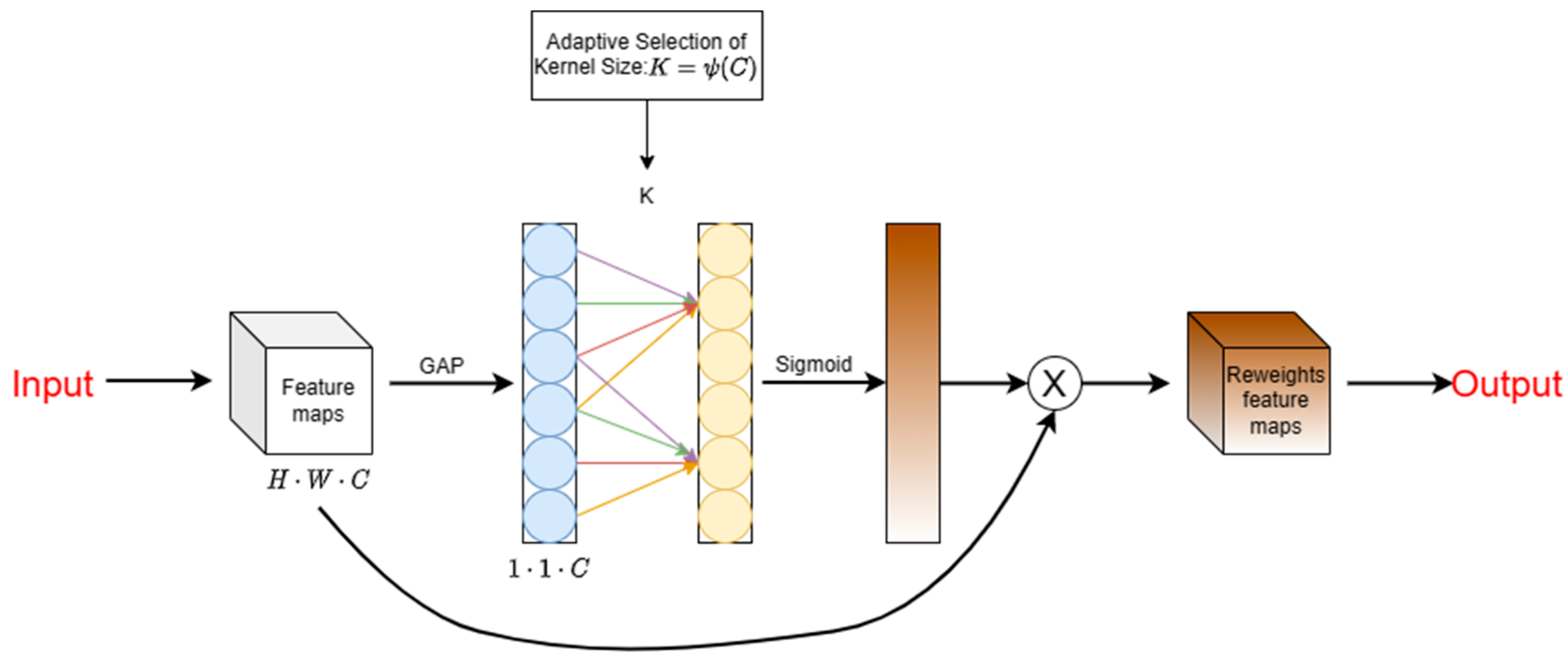
To overcome the trade-off between performance and complexity, this paper adopted an efficient channel attention (ECA) module, which involved only a small number of parameters while achieving significant performance gains. The structure of this module is shown in Figure 4. Without a dimensionality reduction, the ECA module captures local cross-channel interactions by considering each channel and the convolution kernel size, k, after performing the global average pooling step. This approach, compared to dimensionality reduction operations, achieves better results with lower complexity. Here, the convolution kernel size represents the coverage range of local cross-channel interactions.
To avoid manually adjusting the convolution kernel size, k, an adaptive method was employed to determine its size, as shown in Equation (17), allowing the coverage of interactions (i.e., kernel size) to be proportional to the channel size. Consequently, k was adaptively determined through mapping from the vector channel dimension, C. In the proposed health status recognition model, this module reweighted the feature map outputted by the MLFE in the channel dimension, enhancing the sensitivity to fault features and suppressing irrelevant features, thus improving the accuracy of the health status recognition.
k = | log 2 ( C ) γ + b β | o d d
where odd represents the closest odd number, γ and β are set to 2 and 1, respectively, and C represents the number of channels.

3.3. The Proposed Network Structure

The intelligent diagnostic network architecture constructed in this study is shown in Table 1. Due to the lack of consideration for different scale feature maps in the original capsule network, it was necessary to recognize the complex structural features of the machinery equipment for the health state identification. This led to the presence of signals with different fault frequencies and irregular noises in the collected signals. The irregular noise was preliminarily separated using the signal processing method proposed in this article. However, special attention still needed to be paid to the different scale fault features of the signals. Therefore, the main idea behind constructing this model in this study was to extract feature maps of different sizes through the proposed MLFE module and concatenate these feature maps in the channel direction to form a feature map containing different-sized features. Then, this feature map was passed through the ECA module to assign different weights to different-sized features, thereby enhancing the importance of relevant features and suppressing irrelevant features, improving the fault diagnostic performance.
The MLFE module mainly consisted of four convolutional layers, two max-pooling layers, four upsampling layers, and a fusion layer. The convolutional layers had kernel sizes of 64, 128, 256, and 256, all with a kernel size of 3 and a stride of 2. In the max-pooling layers, the pool size and stride were both set to 2. Between the convolutional and pooling layers, the ReLU layer was used to introduce nonlinearity between the layers, addressing the gradient vanishing problem and maintaining the model’s convergence in a stable state.
To address the issue of the mismatched sizes of feature maps, different upsampling factors were used for feature maps of different sizes. Following the MLFE module, the ECA module was employed to adaptively reweight the feature maps of different sizes. Finally, the reweighted feature maps were fed into the capsule network for classification.
During the training process, the model’s loss function was a mixture of the capsule network’s reconstruction loss and margin loss. The training was conducted using a batch size of 5. The Adam optimizer was employed for updating the model parameters in the backward pass, with the learning rate of Adam as:
l r = { 0.001 , 0 N < e 0.5 N 0.0001 , 0.5 N < e 0.8 N 0.00001 , 0.8 N < e N
where N is the preset total iterations number, which is set to 30; e represents the current iteration number. When e is small, a larger lr can speed up the model convergence, while a smaller lr can stabilize the model in the later stages of training.

4. The Proposed Technological Framework

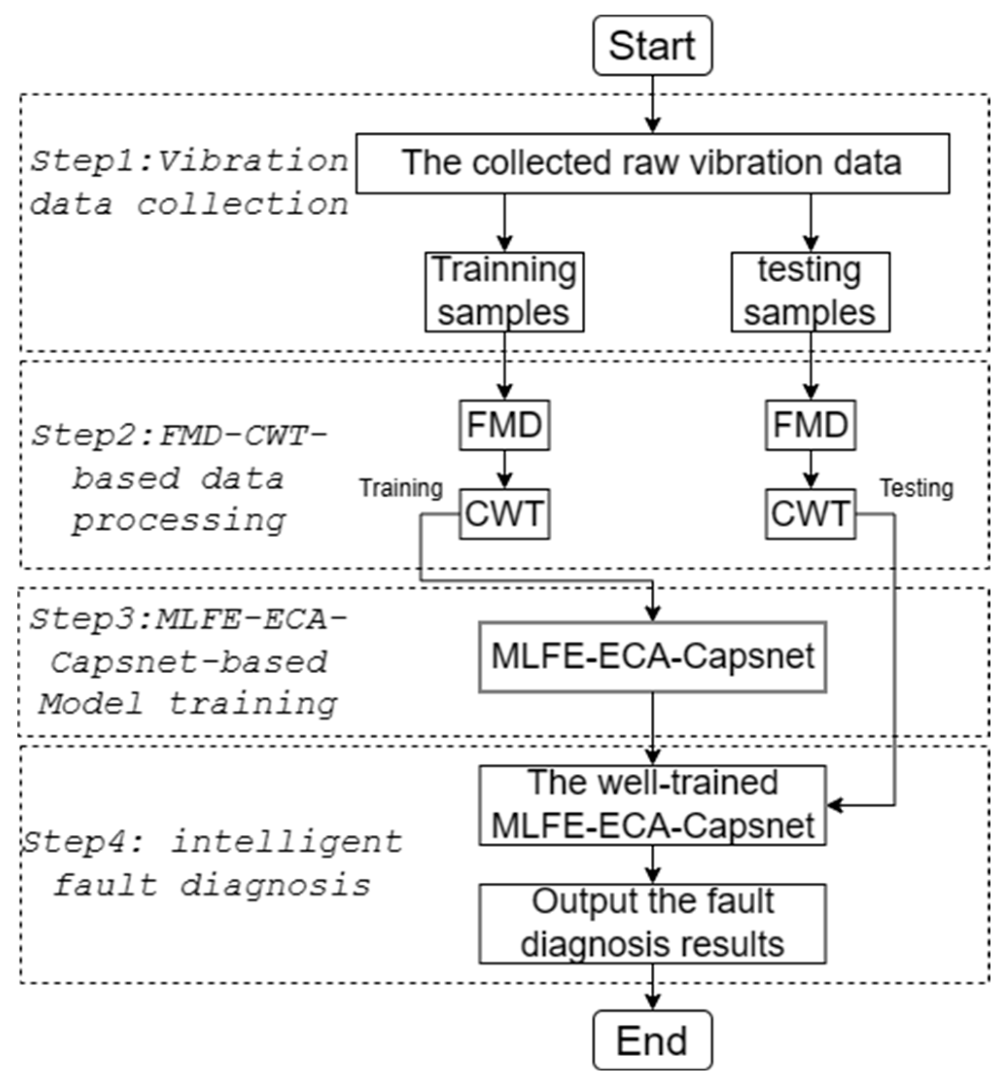
To obtain more discriminative feature information and improve the identification accuracy, an efficient intelligent identification method for the health status of the joint module of an unmanned platform based on the FMD and MLFE-ECA-Capsnet was proposed. The overall diagnostic process was divided into four stages: vibration data acquisition, data processing based on FMD-CWT, model training based on MLFE-ECA-Capsnet, and intelligent fault diagnosis. Figure 5 shows the entire flowchart of the proposed fault diagnosis framework. The specific steps of our method can be summarized as follows:
(1)
Vibration data collection. Firstly, the vibration data of the joint module of the unmanned platform were collected through an accelerometer installed on the upper end of the module’s casing.
(2)
Data processing based on FMD-CWT. The collected vibration data were processed through the FMD to extract effective signal components. The extracted components were then transformed into two-dimensional RGB images containing signal time–frequency features using the CWT. These data were then randomly divided into training and testing samples in a certain proportion.
(3)
Model training based on MLFE-ECA-Capsnet. The training samples were input into the MLFE-ECA-Capsnet for model training, utilizing the adaptive optimizer Adam and L2 regularization to optimize the training process and alleviate overfitting during model training.
(4)
Intelligent fault diagnosis. The testing samples were input into the trained MLFE-ECA-Capsnet to achieve the automatic fault recognition of mechanical faults and output the final diagnostic results.

5. Experimental Verification

The effectiveness of the method for the fault diagnosis of the joint module of unmanned platforms was verified through laboratory experiments. In addition, a comparative analysis was conducted with existing popular methods to validate the advantages of the proposed method. This article concludes with a discussion and outlook.

5.1. Experimental Platform and Data Preparation

5.1.1. Experiment and Dataset Construction

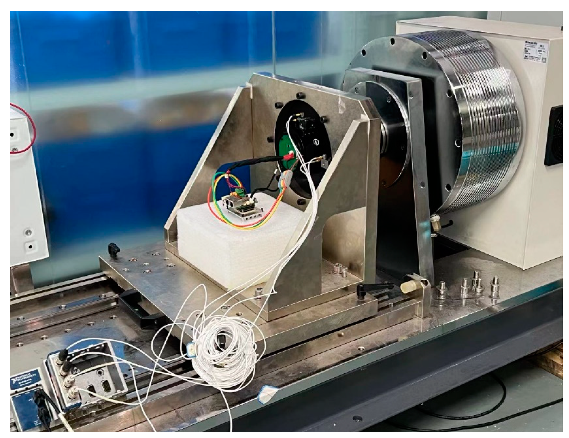
In order to verify the effectiveness of the multi-sensor intelligent diagnosis framework proposed in this section, a simulated experimental platform for the joint module of unmanned platforms was constructed, and relevant signals were collected. As shown in Figure 6, the simulated experimental platform is driven by a motor and the rotating speed can be controlled by a frequency converter. The intermediate transmission part consists of a high-speed stage planetary gearbox and a low-speed stage planetary gearbox. An accelerometer (DYTRAN) used for measuring vibration signals was arranged in a direction perpendicular to the axis on the flange disk of the joint module. During the experiment, the motor speed was set to 2600 r/min and the sampling frequency was 25.6 kHz.
During the experiment, a total of 6 types of experimental data under different health conditions were collected, including normal state (NOR), high-speed stage gear tooth missing (HSGTM), high-speed stage planetary carrier-bearing inner race fault (HSPBIRF), high-speed stage planetary carrier-bearing outer race fault (HSPBORF), high-speed stage planetary carrier-bearing cage fault (HSPBCF), and low-speed stage gear tooth missing (LSGTM). In the experiment, there were 100 samples for each condition. The ratio of the training, validation, and test sets was 0.7:0.1:0.2, as shown in Table 2.

5.1.2. Time–Frequency Representation

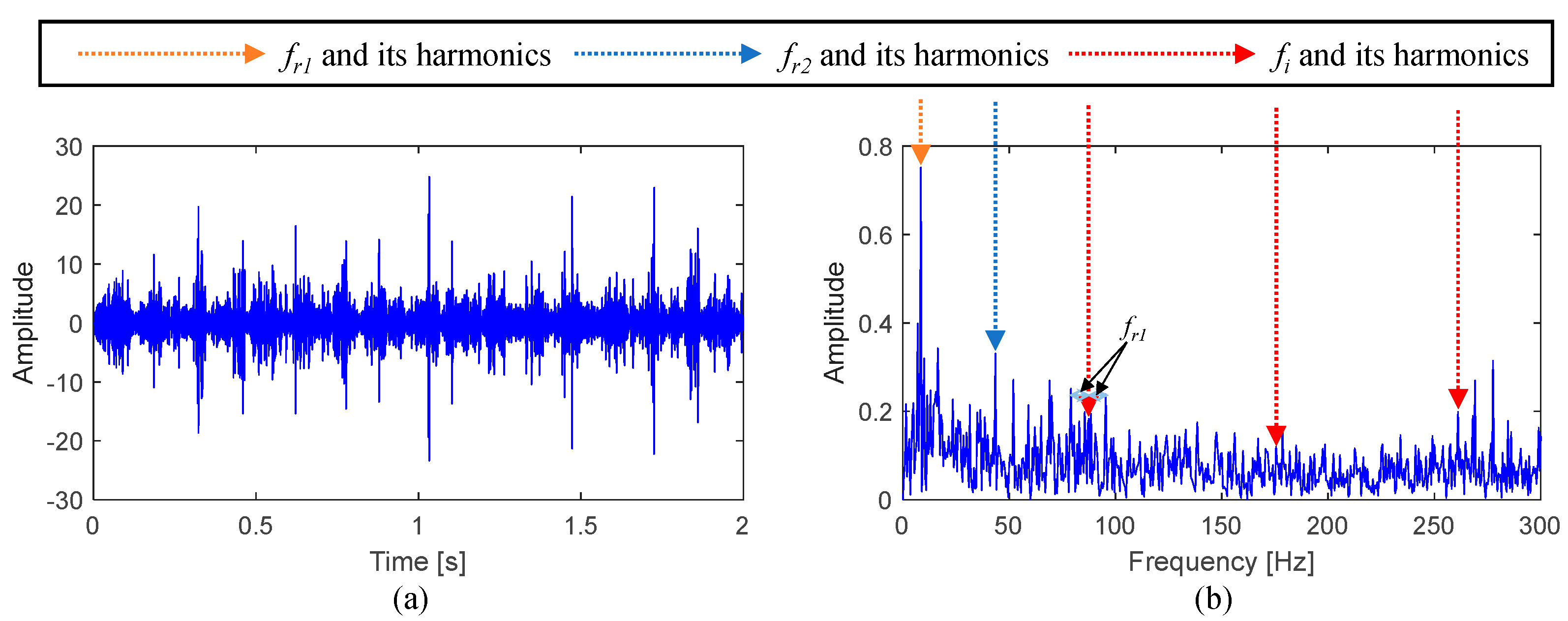
Table 3 shows the rotational frequency of the experimental platform at the experimental speed and the fault frequencies of the planetary carrier-bearing inner and outer races. Figure 7 shows the original signal of the inner race fault. It is difficult to identify the impact features in the time domain from Figure 7a, and also challenging to find any fault information in Figure 7b. Therefore, it was hard to determine whether the bearing was damaged using only the original signal analysis. By using FMD processing on the vibration signal of the inner race fault as shown in Figure 7a, where the FMD modulus and filter length are set to 1 and 40, the decomposition result of the FMD is shown in Figure 8. It is clear from Figure 8a that relevant impact components can be observed. Figure 8b displays the envelope spectrum of the decomposed modal components. The fault frequency, fi, and its harmonics can be clearly observed in Figure 8b, indicating the presence of an inner race fault in the bearing of the joint module of the unmanned platform. This detection result is consistent with the actual situation of the experimental platform. Therefore, the FMD method can effectively remove interference components and extract richer fault information.
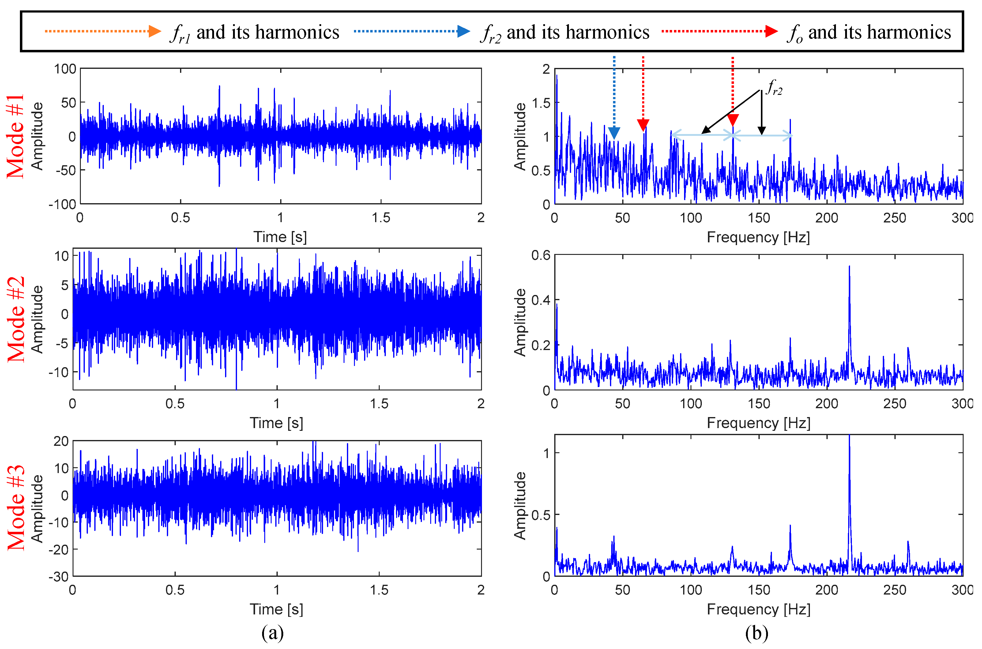
Figure 9 shows the raw signal of the outer race fault. Due to noise interference, it is difficult to observe the relevant frequency of the outer race fault in Figure 9. Therefore, efficient signal processing techniques are needed. The outer race fault vibration signal is processed using the FMD method, as shown in Figure 10a, where the FMD modulus and filter length are set to 3 and 20, respectively. Figure 10 shows the decomposition result of the FMD. In the first modal component, we can clearly see the characteristic frequency of the outer race fault, fo, and its harmonic components.
In order to demonstrate the superiority of the feature modal decomposition (FMD) method compared to other signal decomposition algorithms, this study employed the comprehensive index (CI) (see Equation (19)) for a quantitative assessment of the decomposition performance of each algorithm. CI is defined as the product of the average slope at each order and the ratio of average feature energy, providing a comprehensive evaluation metric for the efficiency of each method.
C I = K u r m × F E R m
K u r m = 1 N n = 1 N ( u m ( n ) u ¯ m ( n ) ) 4 σ 4 , F E R m = A ( f ) + A ( 2 f ) + A ( 3 f ) A t o t a l
where K u r m and F E R m represent the kurtosis and feature energy ratio of the m-th mode component, respectively; N denotes the signal length; u ¯ m ( k ) and σ are the mean and standard deviation of the m-th mode component, respectively; f denotes the fault frequency; A(f), A(2f), and A(3f) are the amplitudes corresponding to the envelope spectrum’s first three harmonic frequencies; and Atotal is the total amplitude of the envelope spectrum. CI can concurrently assess the impulsiveness and cyclostationarity of the mode components, with larger CI values indicating a better decomposition performance. Table 4 presents the decomposition results of three methods (i.e., EEMD, VMD, and FMD) for the outer ring signal. Apparently, compared with EEMD and VMD, the CI value of the FMD is basically the largest in each order mode component, except for #2 mode components.
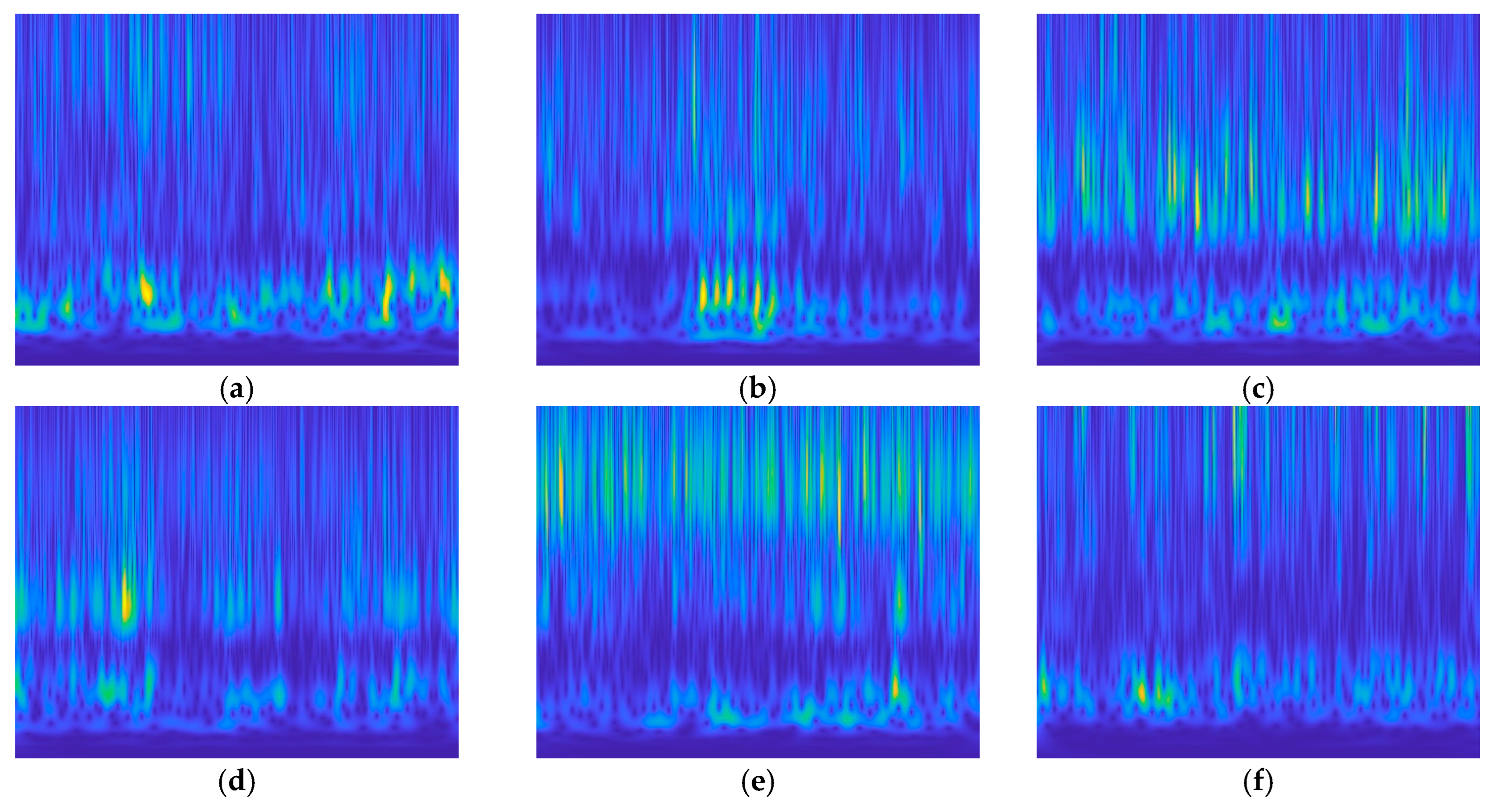
Figure 11 and Figure 12 show the time–frequency diagrams of various health states obtained before and after using the FMD for signal processing with the continuous wavelet transform. It is evident from the figures that the time–frequency diagram of the signal processed with the FMD method removes the interfering components, making the fault characteristics more prominent. This directly enhances the diagnostic performance of the fault diagnosis model.

5.2. Effectiveness Verification of the FMD Method

To illustrate the effectiveness of the data processing methods used, the data before and after being processed by the FMD were used in the MLEF-ECA-Capsnet for fault diagnosis in the same proportion. Ultimately, the changes in the loss value and accuracy during the training process were compared. The changes in the loss value and classification accuracy during the model training process are shown in Figure 13. From the perspective of the loss value, the trend of the loss value change in the dataset before and after FMD processing was similar, but the processed data showed a faster convergence speed. In terms of accuracy, the data processed with the FMD method clearly exhibit more prominent fault characteristics compared to the data before processing, and they can make the model more stable and accurate during the training process.
The confusion matrices of the classification results on the test set for these four models are shown in Figure 14. It can be seen that the model trained on the dataset before FMD processing achieves an accuracy of only 97.5% on the test set. In contrast, the model trained on the dataset after FMD processing achieves 100% accuracy on the test set. The experimental results indicate that preprocessing vibration data with the FMD can effectively improve the diagnostic performance of the fault diagnosis model.

5.3. Ablation Analysis

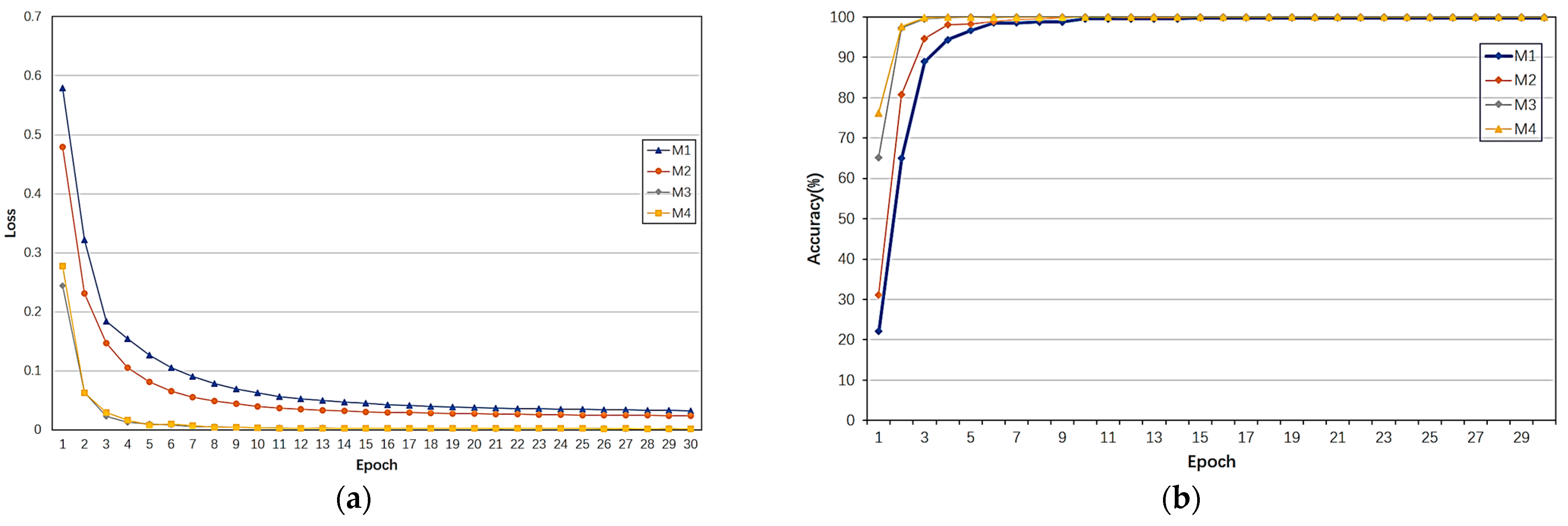
To illustrate the effectiveness of the proposed feature enhancement network, four classification models were designed for comparison: (1) original CapsNet (M1); (2) CapsNet with an ECA module (M2); (3) CapsNet with an MLFE module (M3); and (4) the proposed MLFE-ECA-CapsNet (M4). From Table 5, it can be observed that, compared to the original CapsNet model, the increases in parameters and time consumption caused by the ECA module are less than that of the MLFE module. The changes in the loss value and classification accuracy during the model training process are shown in Figure 15. In terms of the loss value, M1 has the largest variation, followed by M2. The variation trends of M3 and M4 are similar, but the stable loss value on the validation set of M4 is slightly lower than that of M3. In terms of accuracy, when the number of training iterations is small, M1 has the lowest training accuracy and M4 has the highest training accuracy. Compared to M1, the performances of M2 and M3 are improved to varying degrees, with M3 showing the most significant improvement. The performance of M3 is the most similar to M4, but M4 converges faster than M3, and with an increase in training cycles, the accuracy of M3 fluctuates to some extent, while the accuracy of M4 is relatively stable.
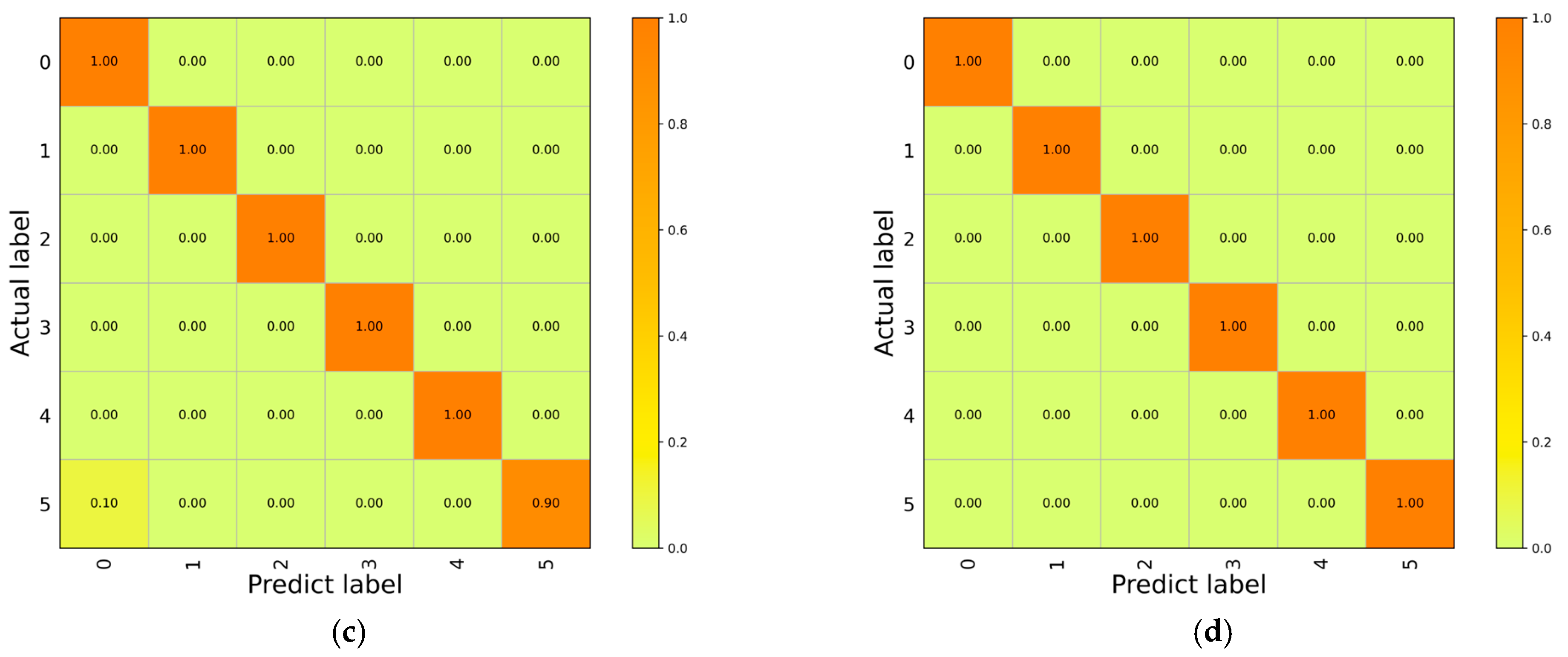
The confusion matrix of the classification results on the test set for these four models is shown in Figure 16. It can be observed that in M1, M2, and M3, 3, 2, and 1 test samples, respectively, are misclassified as other types, while M4 classifies all samples correctly. The experimental results indicate that this feature enhancement network can effectively improve the fault-sensitive feature-mining capability and diagnostic performance of the CapsNet classifier. Both modules show corresponding improvements in classification performance and stability. Although the MLFE module increases the time consumption, it is still acceptable given its role in improving the stability and accuracy of the model. The experimental results indicate that the MLFE module shows the greatest improvement for both the classification accuracy and stability of the original Capsnet model. Although the ECA module also improves the original model to some extent in situations with fewer feature channels, the accuracy and stability of the improved model (i.e., M2) are closer to the original model. Therefore, based on the loss and accuracy changes in different models during the training process and the confusion matrix of the final classification results obtained in this experiment, the following conclusions can be drawn: (1) the MLFE module plays a major role in improving the original model; (2) the ECA module can only have a certain effect on large-scale models with multiple scales; and (3) the MLFE and ECA modules complement each other, leading to a significant improvement in the classification performance of Capsnet.

5.4. Network Comparisons

To validate the superior performance of the MLFE-ECA-Capsnet network model proposed in this paper, its results for the intelligent diagnosis of unmanned platform joint modules are compared and studied with the analysis results of other advanced deep neural network models. These network models are Resnet50 [33], VGG19 [34], and Densenet121 [35]. The Resnet50 network contains 49 convolutional layers and one fully connected layer, with its key component being the residual structure, which can solve the gradient problem. The increase in the number of network layers also improves the expression of features and consequently enhances the performances of detection or classification. In addition, the use of 1 × 1 convolutions in the residual structure can reduce the parameter quantity and, to some extent, the computational load. VGG19 network comprises 16 convolutional layers and 3 fully connected layers. For a given receptive field, VGG19 uses stacked small convolutional kernels instead of large ones because multiple non-linear layers can increase the network depth to ensure the learning of more complex patterns, with fewer parameters. Densenet121 consists of four dense blocks and one transition layer, achieving efficient feature propagation and reuse through the combination of dense connections and transition layers, reducing the number of parameters and computational load, and achieving a good performance in many image classification tasks. When comparing the abovementioned four network models, the input for all was the time–frequency map, with the training cycles set to 100 for Resnet50 and VGG19, and 50 for Densenet121, while other hyperparameters remained consistent with the proposed network model.
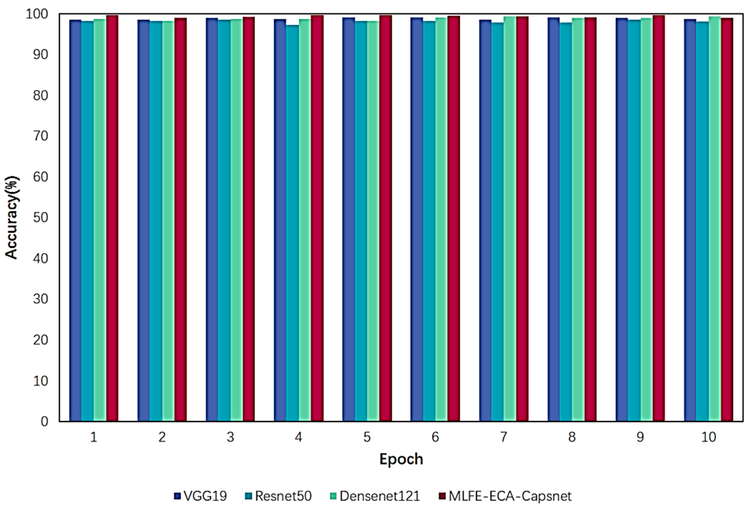
To demonstrate the advantages and stability of the proposed method in the intelligent diagnosis of voltage signals, ten experiments were conducted using other advanced models and the proposed method. Figure 17 and Table 6 present the ten diagnostic results of different models, indicating that the feature-enhanced diagnostic model proposed in this paper has the best diagnostic effect. The highest accuracy for the ten results is 100%, the lowest accuracy is 99.33%, and the average accuracy on the test set can reach 99.61%, with the smallest variance, indicating that the proposed method has the best stability. Among other classification models, Densenet121 has the highest diagnostic accuracy, with an average accuracy of 98.88% on the test set. The worst diagnostic performance is by Resnet50, with the highest accuracy in the ten results being 98.54%, the lowest accuracy being only 97.29%, and the average accuracy being 98.16%, which is 1.45% lower than the proposed method, and the standard deviation is the highest, indicating the worst stability. The results above indicate that, compared with other advanced deep neural network methods, the feature-enhanced diagnostic model proposed in this paper has a superior diagnostic performance and good stability.
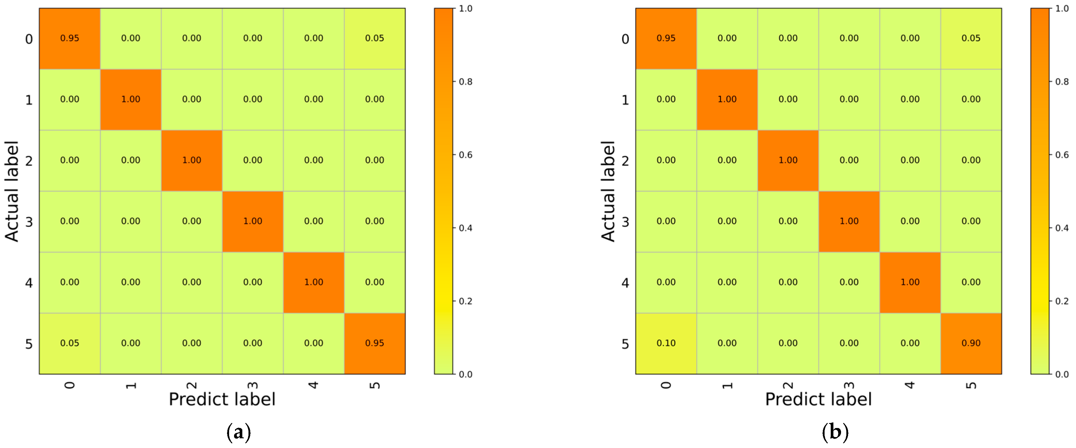
Figure 18 shows the confusion matrix of different methods on the test set. From the figure, it can be observed that the proposed method has an excellent diagnostic performance compared to other deep neural network models. The VGG19 model incorrectly classified a total of nine test set samples into other healthy states, including four samples with a label of 0, one sample with a label of 2, three samples with a label of 6, and one sample with a label of 11. The Resnet50 model incorrectly classified four samples with a label of 0 into other healthy states. The Densenet121 model incorrectly classified four samples with a label of 0 and two samples with a label of 11 into other healthy states. In contrast, the proposed method performed excellently on the test set, with only one sample being misclassified. These results indicate that, compared to other deep neural network models, the feature-enhanced diagnostic model proposed in this paper demonstrates a superior diagnostic performance and robustness.

6. Conclusions

This study proposed an intelligent diagnosis model of a reinforced capsule network based on a multi-scale feature enhancement module and efficient channel attention module for the efficient intelligent identification of the health status of unmanned platform joint modules. Firstly, the collected time-domain vibration signals were filtered using the FMD and then transformed into time–frequency maps with two-dimensional features through the continuous wavelet transform based on the Morlet wavelet as the input to the neural network. In the fault diagnosis stage, the MLFE module, which fused feature maps of different scales in the feedforward process, and the ECA module, which obtained an adaptive interaction range with adaptive convolution kernels, enhanced the key channel features while suppressing irrelevant features. Then, the obtained feature maps were input into the capsule network to convert scalars into vectors, further obtaining detailed information of the features, and finally the vector length output by the main capsule layer was transformed into the diagnosis result. This method not only improved the diagnostic performance of the diagnostic model, but also prevented problems such as the excessively long training time and overfitting caused by overly complex network structures. The effectiveness of the proposed method was verified using vibration signals collected from a simulated test bench of the joint module of an unmanned platform. The experimental results show that the proposed feature-enhanced intelligent diagnosis framework has a high recognition accuracy. The specific conclusions are as follows:
(1)
The time–frequency representation achieved through the continuous wavelet transform based on Morlet after filtering by the FMD method can obtain richer time-domain and frequency-domain information compared to the original time-domain signal, which is beneficial for the diagnostic performance of the diagnostic model.
(2)
Compared with the original capsule network, the MLFE and ECA modules included in the proposed method have different degrees of improvement for the original capsule network, with the MLFE module having the greatest improvement, but with increased parameters and training times. Overall, the proposed method is a good improvement compared to the original capsule network.
(3)
Compared with other advanced diagnostic networks, the proposed feature-enhanced diagnostic model exhibits a good performance in terms of its diagnostic accuracy and diagnostic stability, which also proves the effectiveness of the two proposed modules.
In practical engineering scenarios, acquiring a large amount of labeled fault data is extremely difficult, which remains a major challenge in the development of state recognition. Furthermore, the complex structure of actual engineering machinery leads to the complexity of collected signal components and the presence of a large amount of noise. Therefore, an effective signal processing method for extracting key fault information is particularly important and should be a focus of the future research in this field. Additionally, training neural network models requires significant computational resources. Exploring how to utilize pre-training strategies to reduce the time cost of data processing and ensure diagnostic accuracy are also issues that need to be addressed in future studies.

Author Contributions

Data curation, S.Z., S.S. and R.D.; investigation, S.Z., H.Y. and S.S.; supervision, G.Y. All authors have read and agreed to the published version of the manuscript.

Funding

This research was funded by the Key Research and Development Program of Sichuan Province under grant number 2021YFG0076.

Data Availability Statement

Data are contained within the article.

Conflicts of Interest

The authors declare no conflict of interest.

References

  1. Hu, X.; Assaad, R.H. The use of unmanned ground vehicles (mobile robots) and unmanned aerial vehicles (drones) in the civil infrastructure asset management sector: Applications, robotic platforms, sensors, and algorithms. Expert Syst. Appl. 2023, 232, 120897. [Google Scholar] [CrossRef]
  2. Laghari, A.A.; Jumani, A.K.; Laghari, R.A.; Nawaz, H. Unmanned aerial vehicles: A review. Cogn. Robot. 2023, 3, 8–22. [Google Scholar] [CrossRef]
  3. Xia, B.; Wang, K.; Xu, A.; Zeng, P.; Yang, N.; Li, B. Intelligent Fault Diagnosis for Bearings of Industrial Robot Joints Under Varying Working Conditions Based on Deep Adversarial Domain Adaptation. IEEE Trans. Instrum. Meas. 2022, 71, 1–13. [Google Scholar] [CrossRef]
  4. Pan, J.; Qu, L.; Peng, K. Deep residual neural-network-based robot joint fault diagnosis method. Sci. Rep. 2022, 12, 17158. [Google Scholar] [CrossRef] [PubMed]
  5. Li, Y.; Cheng, G.; Liu, C. Research on bearing fault diagnosis based on spectrum characteristics under strong noise interference. Measurement 2021, 169, 108509. [Google Scholar] [CrossRef]
  6. Yan, R.; Shang, Z.; Xu, H.; Wen, J.; Zhao, Z.; Chen, X.; Gao, R. Wavelet transform for rotary machine fault diagnosis:10 years revisited. Mech. Syst. Signal Process. 2023, 200, 110545. [Google Scholar] [CrossRef]
  7. Sylvain, M.; Duong-Hung, P.; Marcelo, A. On the use of short-time fourier transform and synchrosqueezing-based demodulation for the retrieval of the modes of multicomponent signals. Signal Process. 2021, 178, 107760. [Google Scholar]
  8. Cui, H.; Guan, Y.; Deng, W. Fault Diagnosis Using Cascaded Adaptive Second-Order Tristable Stochastic Resonance and Empirical Mode Decomposition. Appl. Sci. 2021, 11, 11480. [Google Scholar] [CrossRef]
  9. Yin, C.; Wang, Y.; Ma, G.; Wang, Y.; Sun, Y.; He, Y. Weak fault feature extraction of rolling bearings based on improved ensemble noise-reconstructed EMD and adaptive threshold denoising. Mech. Syst. Signal Process. 2022, 171, 108834. [Google Scholar] [CrossRef]
  10. Li, Z.; Chen, J.; Zi, Y.; Pan, J. Independence-oriented VMD to identify fault feature for wheel set bearing fault diagnosis of high speed locomotive. Mech. Syst. Signal Process. 2017, 85, 512–529. [Google Scholar] [CrossRef]
  11. Yu, J.; Lv, J. Weak Fault Feature Extraction of Rolling Bearings Using Local Mean Decomposition-Based Multilayer Hybrid Denoising. IEEE Trans. Instrum. Meas. 2017, 66, 3148–3159. [Google Scholar] [CrossRef]
  12. Pan, H.; Yang, Y.; Li, X.; Zheng, J.; Cheng, J. Symplectic geometry mode decomposition and its application to rotating machinery compound fault diagnosis. Mech. Syst. Signal Process. 2019, 114, 189–211. [Google Scholar] [CrossRef]
  13. Chen, Y.; Zhang, T.; Zhao, W.; Luo, Z.; Lin, H. Rotating Machinery Fault Diagnosis Based on Improved Multiscale Amplitude-Aware Permutation Entropy and Multiclass Relevance Vector Machine. Sensors 2019, 19, 4542. [Google Scholar] [CrossRef]
  14. Miao, Y.; Zhang, B.; Li, C.; Lin, J.; Zhang, D. Feature Mode Decomposition: New Decomposition Theory for Rotating Machinery Fault Diagnosis. IEEE Trans. Ind. Electron. 2023, 70, 1949–1960. [Google Scholar] [CrossRef]
  15. Li, L.; Meng, W.; Liu, X.; Fei, J. Research on Rolling Bearing Fault Diagnosis Based on Variational Modal Decomposition Parameter Optimization and an Improved Support Vector Machine. Electronics 2023, 12, 1290. [Google Scholar] [CrossRef]
  16. Zhang, S.; Xu, F.; Hu, M.; Zhang, L.; Liu, H.; Li, M. A novel denoising algorithm based on TVF-EMD and its application in fault classification of rotating machinery. Measurement 2021, 179, 109337. [Google Scholar] [CrossRef]
  17. Jin, Z.; He, D.; Ma, R.; Zou, X.; Chen, Y.; Shan, S. Fault diagnosis of train rotating parts based on multi-objective VMD optimization and ensemble learning. Digit. Signal Process. 2022, 121, 103312. [Google Scholar] [CrossRef]
  18. Tong, Q.; Cao, J.; Han, B.; Zhang, X.; Nie, Z.; Wang, J.; Lin, Y.; Zhang, W. A Fault Diagnosis Approach for Rolling Element Bearings Based on RSGWPT-LCD Bilayer Screening and Extreme Learning Machine. IEEE Access 2017, 5, 5515–5530. [Google Scholar] [CrossRef]
  19. Tu, Z.; Gao, L.; Wu, X.; Liu, Y.; Zhao, Z. Rotate Vector Reducer Fault Diagnosis Model Based on EEMD-MPA-KELM. Appl. Sci. 2023, 13, 4476. [Google Scholar] [CrossRef]
  20. Chen, J.; Lin, C.; Yao, B.; Yang, L.; Ge, H. Intelligent fault diagnosis of rolling bearings with low-quality data: A feature significance and diversity learning method. Reliab. Eng. Syst. Saf. 2023, 237, 109343. [Google Scholar] [CrossRef]
  21. Tran, M.; Liu, M.; Tran, Q.; Nguyen, T. Effective Fault Diagnosis Based on Wavelet and Convolutional Attention Neural Network for Induction Motors. IEEE Trans. Instrum. Meas. 2022, 71, 1–13. [Google Scholar] [CrossRef]
  22. Zaman, W.; Ahmad, Z.; Siddique, M.F.; Ullah, N.; Kim, J.-M. Centrifugal Pump Fault Diagnosis Based on a Novel SobelEdge Scalogram and CNN. Sensors 2023, 23, 5255. [Google Scholar] [CrossRef]
  23. Tang, S.; Zhu, Y.; Yuan, S. Intelligent fault identification of hydraulic pump using deep adaptive normalized CNN and synchrosqueezed wavelet transform. Reliab. Eng. Syst. Saf. 2022, 224, 108560. [Google Scholar] [CrossRef]
  24. Huang, D.; Zhang, W.; Guo, F.; Liu, W.; Shi, X. Wavelet Packet Decomposition-Based Multiscale CNN for Fault Diagnosis of Wind Turbine Gearbox. IEEE Trans. Cybern. 2023, 53, 443–453. [Google Scholar] [CrossRef] [PubMed]
  25. Xiong, J.; Liu, M.; Li, C.; Cen, J.; Zhang, Q.; Liu, Q. A Bearing Fault Diagnosis Method Based on Improved Mutual Dimensionless and Deep Learning. IEEE Sens. J. 2023, 23, 18338–18348. [Google Scholar] [CrossRef]
  26. Zhang, H.; Shi, P.; Han, D.; Jia, L. Research on rolling bearing fault diagnosis method based on AMVMD and convolutional neural networks. Measurement 2023, 217, 113028. [Google Scholar] [CrossRef]
  27. Kim, Y.; Na, K.; Youn, B. A health-adaptive time-scale representation (HTSR) embedded convolutional neural network for gearbox fault diagnostics. Mech. Syst. Signal Process. 2022, 167, 108575. [Google Scholar] [CrossRef]
  28. Zhang, Y.; Liu, W.; Wang, X.; Gu, H. A novel wind turbine fault diagnosis method based on compressed sensing and DTL-CNN. Renew. Energy 2022, 194, 249–258. [Google Scholar] [CrossRef]
  29. Gu, J.; Peng, Y.; Lu, H.; Chang, X.; Chen, G. A novel fault diagnosis method of rotating machinery via VMD, CWT and improved CNN. Measurement 2022, 200, 111635. [Google Scholar] [CrossRef]
  30. Xie, F.; Li, G.; Song, C.; Song, M. The Early Diagnosis of Rolling Bearings’ Faults Using Fractional Fourier Transform Information Fusion and a Lightweight Neural Network. Fractal Fract. 2023, 7, 875. [Google Scholar] [CrossRef]
  31. Liang, P.; Deng, C.; Yuan, X.; Zhang, L. A deep capsule neural network with data augmentation generative adversarial networks for single and simultaneous fault diagnosis of wind turbine gearbox. ISA Trans. 2023, 135, 462–475. [Google Scholar] [CrossRef] [PubMed]
  32. Siddique, M.F.; Ahmad, Z.; Kim, J.-M. Pipeline leak diagnosis based on leak-augmented scalograms and deep learning. Eng. Appl. Comput. Fluid Mech. 2023, 17, 1. [Google Scholar] [CrossRef]
  33. He, K.; Zhang, X.; Ren, S.; Sun, J. Deep Residual Learning for Image Recognition. In Proceedings of the 2016 IEEE Conference on Computer Vision and Pattern Recognition (CVPR), Las Vegas, NV, USA, 27–30 June 2016; pp. 770–778. [Google Scholar]
  34. Santos, F.; Santos, E.; Vogado, L.; Ito, M.; Bianchi, A.; Tavares, J.; Veras, R. DFU-VGG, a Novel and Improved VGG-19 Network for Diabetic Foot Ulcer Classification. In Proceedings of the 2022 29th International Conference on Systems, Signals and Image Processing (IWSSIP), Sofia, Bulgaria, 1–3 June 2022; pp. 1–4. [Google Scholar]
  35. Huang, G.; Liu, Z.; Maaten, L.; Weinberger, K. Densely Connected Convolutional Networks. In Proceedings of the 2017 IEEE Conference on Computer Vision and Pattern Recognition (CVPR), Honolulu, HI, USA, 21–26 July 2017; pp. 2261–2269. [Google Scholar]
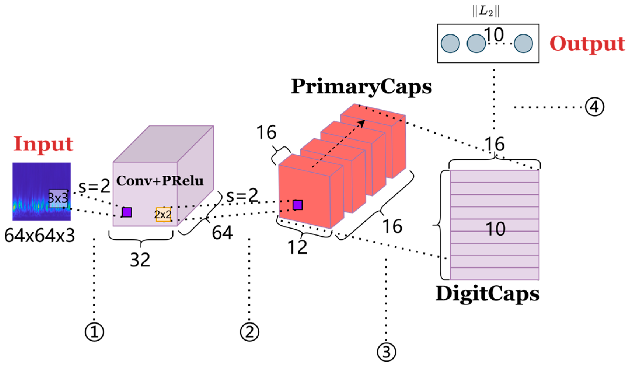
Figure 1. Capsule network structure diagram.
Machines 12 00079 g001
Figure 2. Capsule networks use dynamic routing algorithms to improve the efficiency of routing information through the network.
Machines 12 00079 g002
Figure 3. Structure of the MLFE module.
Machines 12 00079 g003
Figure 4. Structure of the ECA module.
Machines 12 00079 g004
Figure 5. The flowchart of the proposed technological framework.
Machines 12 00079 g005
Figure 6. Simulated experimental platform for the joint module of unmanned platforms.
Machines 12 00079 g006
Figure 7. The vibration signals of the inner race fault in the (a) time domain and (b) its envelope spectrum.
Machines 12 00079 g007
Figure 8. (a) FMD decomposition mode and (b) its envelope spectrum.
Machines 12 00079 g008
Figure 9. (a) Time domain of the outer race fault vibration signal and (b) its envelope spectrum.
Machines 12 00079 g009
Figure 10. (a) FMD decomposition mode and (b) its envelope spectrum.
Machines 12 00079 g010
Figure 11. Time–frequency diagrams created after the original signal is transformed by the CWT. (a) HSPBCF, (b) HSGTM, (c) HSPBIRF, (d) LSGTM, (e) NOR, (f) HSPBORF.
Machines 12 00079 g011
Figure 12. Time–frequency diagrams created after the signal processed by the FMD is transformed by the CWT. (a) HSPBCF, (b) HSGTM, (c) HSPBIRF, (d) LSGTM, (e) NOR, (f) HSPBORF.
Machines 12 00079 g012aMachines 12 00079 g012b
Figure 13. Changes in loss value and accuracy of different data during the training process. (a) Loss value variation; (b) accuracy variation.
Machines 12 00079 g013
Figure 14. The confusion matrices of the classification results on the test set before and after using the FMD for signal processing. (a) Original signal; (b) signal after FMD processing.
Machines 12 00079 g014
Figure 15. Changes in loss value and accuracy of different models during the training process. (a) Loss value variation; (b) accuracy variation.
Machines 12 00079 g015
Figure 16. Confusion matrix of the classification results for the test set. (a) M1, (b) M2, (c) M3, (d) M4.
Machines 12 00079 g016aMachines 12 00079 g016b
Figure 17. Diagnostic results of ten training sessions for different methods.
Machines 12 00079 g017
Figure 18. Confusion matrix of the test set for different methods. (a) VGG19, (b) Resnet50, (c) Densenet121, (d) MLFE-ECA-Capsnet.
Machines 12 00079 g018aMachines 12 00079 g018b
Table 1. Model structure of the proposed intelligent diagnosis method.
LayersTypesOutput SizeLast Layer
InputInput layerInput(64,64,3)\
MLFE moduleConv1Conv(64,3,2)(32,32,64)Input layer
Activation1Relu(32,32,64)Conv1
Conv2Conv(128,3,2)(16,16,128)Activation1
Activation 2Relu(16,16,128)Conv2
Pooling1MaxPool(2,2)(8,8,128)Activation 2
Conv3Conv(256,3,2)(4,4,256)Pooling1
Activation 3Relu(4,4,256)Conv3
Conv4Conv(512,3,2)(2,2,512)Activation 3
Activation 4Relu(2,2,512)Conv4
Pooling2MaxPool(2,2)(1,1,512)Activation 4
Upsamlping1Upsampling(2,2)(32,32,128)Pooling2
Upsamlping2Upsampling(4,4)(32,32,128)Upsamlping1
Upsamlping3Upsampling(16,16)(32,32,512)Upsamlping2
Upsamlping4Upsampling(32,32)(32,32,512)Upsamlping3
Fusion1Contact(32,32,1280)Upsamlping4
BN1BN(32,32,1280)Fusion1
Activation 5Relu(32,32,1280)BN1
ECA modulePooling3GAP(1280)Activation 5
Reshape1Reshape(1,1,1280)Pooling3
Conv5Conv(2,2,1)(1,1,1)Reshape1
Activation6Sigmoid(1,1,1)Conv5
Fusion2Multiply(15,15,256)Activation6
Capsule networkPrimary capsulePrimarycap(14,16)Fusion2
Digit capsuleDigitcap(14)Primary capsule
Table 2. Experimental dataset.
LabelTypes of FaultsTraining/Validation/Test Samples
0HSPBCF70/10/20
1HSGTM70/10/20
2HSPBIRF70/10/20
3LSGTM70/10/20
4NOR70/10/20
5HSPBORF70/10/20
Table 3. Comparison of four classification models.
fr1 (Hz)fr2 (Hz)fi (Hz)fo (Hz)
8.5843.3387.7565
Table 4. CI values of each mode component acquired via various approaches.
Different ApproachesMode #1Mode #2Mode #3
FMD0.01090.00380.0073
VMD0.00480.00170.0057
EEMD0.00530.00410.0067
Table 5. Comparison of four classification models.
ModelParameterTraining Time (s)
M118,916,325122.3294
M218,916,608123.5110
M324,617,856200.7728
M424,622,976211.3169
Table 6. Accuracy (%) of ten training sessions for different methods.
ModelHighest ValueMinimum ValueMean ValueStandard Deviation
VGG1999.1698.5498.850.263
Resnet5098.5497.2998.160.378
Densenet12199.3798.3498.880.366
Proposed method10099.3399.610.251
Disclaimer/Publisher’s Note: The statements, opinions and data contained in all publications are solely those of the individual author(s) and contributor(s) and not of MDPI and/or the editor(s). MDPI and/or the editor(s) disclaim responsibility for any injury to people or property resulting from any ideas, methods, instructions or products referred to in the content.