Abstract
Quadrotors possess traits such as under-actuation, nonlinearity, and strong coupling. Quaternions are primarily used for attitude calculations in drones, with error quaternions seldom being employed directly in the control of specific quadcopter drones. This paper focuses on the low tracking accuracy and weak anti-interference ability of quadcopter drones in trajectory-tracking control. By establishing the quadcopter quaternion model, a controller based on quaternion error is designed through a combination of fractional-order PID control with S-plane control. Trajectory-tracking experiments demonstrate that, in comparison with fractional-order PID, this method exhibits strong wind disturbance resistance and high tracking accuracy.
1. Introduction
The quadrotor is an unmanned aerial vehicle with extensive uses in multiple fields. In comparison to other rotorcrafts, the quadrotor boasts a simpler structure and is more commonly used. The aircraft is composed of four rotors that control its flight by regulating the speed of rotation. Additionally, it is compact in size, easy to maintain, highly maneuverable, and considered safe and reliable. The quadrotor is cost-effective and can be accessorized by mechanical arms as per mission requirements.
Despite its extensive use, the quadrotor is a complex system to model and for which to design control systems. This is due to its six-degrees-of-freedom flight control with only four rotor inputs and six-space-degrees-of-freedom outputs, which result in a strongly coupled, underactuated, and nonlinear system.
Based on the above problems, researchers have proposed many control algorithms for quadrotors, such as PID control [1], fractional-order PID control [2], backstepping control [3], active disturbance rejection control [4,5], sliding mode control [6], fuzzy control [7], etc.
Muro et al. [8] proposed a sliding mode control algorithm based on a super twisting algorithm and used unit quaternion feedback in the dynamic model of the quadrotor. The accurate first-order differentiator was used to obtain the derivative of the virtual control input, and the sliding mode observer was used to estimate the aerodynamic forces and moments acting on the quadrotor, ensuring robustness against external disturbance and model uncertainty. The results showed that the control method based on quaternions needed less time than the method using Euler angles.
Chen Pengyun et al. [9] proposed an expert S-plane controller and introduced it to the motion control system of UAVs. The controller, combined with expert control, has a good nonlinear control effect and can achieve good UAV motion control. Based on this, the motion control system of UAV was designed. Field tests showed that the proposed controller has the characteristics of a high control accuracy, fast response speed, good dynamic performance, and strong adaptability to environmental interference, and is suitable for the motion control of UAVs.
P.D. MANDIĆ et al. [10] studied the stability problem of the fractional-order PD controller controlling the Furuta pendulum. The mathematical model of the rotary-inverted pendulum was derived, and the fractional-order PD controller was introduced to stabilize this. Here, the D-decomposition method can be successfully used to solve the asymptotic stability problem of the inverted pendulum system, which is controlled by the fractional-order controller. The fractional-order controller can be applied to underactuated system control.
Liu Tong [11] quoted the fractional-order operator in the fuzzy controller of the quadrotor and constructed an adaptive fuzzy fractional-order PID controller, which is used in the quadrotor control system. The experimental results show that this method has a better control performance compared with PID and fractional-order PID controllers.
Due to the underactuated nature of the quadrotors, the stability of the model and the complexity of the dynamic model become more prominent when subjected to vibration, noise, and interference. In addition, the overlapping of the axes during the high maneuvering of the UAV can cause singularities [12]. In order to address this, Reference [13] suggests using a reverse-saturation, adaptive, fixed-time, sliding-mode controller for second-order nonlinear systems with saturation constraints. This approach involves designing a new, non-singular, fast, fixed-time sliding surface, which helps to avoid singularity and achieve faster convergence rates. Islam et al. [14] used model predictive control (MPC) for the trajectory-tracking control of a quadrotor based on quaternions. A new cost function was developed for the MPC controller using quaternions. The simulation results showed that using the MPC method for quadrotor trajectory tracking can effectively avoid directional singularity. Another option is to utilize quaternions to establish the UAV model. This article demonstrates the effectiveness of using quaternions to directly control specific quadrotor UAVs. To overcome the influence of wind disturbance on quadrotor trajectory-tracking control, a new control method is proposed in this paper. This method is based on traditional PID control and proposes a quadrotor-tracking control method based on fractional-order PID and S-plane. The structure of this paper is as follows: first, according to the force and torque of the quadrotor, the kinematic and dynamic equations of the UAV are established using quaternions. Then, a fractional-order S-plane control is designed. Finally, simulation experiments are carried out using Matlab Simulink.
2. Quaternions Model for Quadrotor UAV
This article describes the motion state of a quadcopter with six degrees of freedom (DOF) and uses the Newton–Euler formula to establish the quadcopter’s kinematic and dynamic models. To establish the kinematic equations, coordinate systems need to be constructed. Therefore, this article constructs the Earth-fixed coordinate system and the body-fixed coordinate system. The Earth-fixed coordinate system is an inertial coordinate system, and the origin of the coordinate system can be set to the initial position at which the quadcopter takes off. The body-fixed coordinate system is a fixed coordinate system, and the origin of the coordinate system is the center of gravity of the quadcopter. The position of the quadcopter can be described by , and the rotation along the axis (i.e., roll, pitch, and yaw) can be represented by .
The transformation matrix between the Earth-fixed coordinate system and the body-fixed coordinate system is Q. Typically, the rotation matrix from the Earth-fixed coordinate system to the body-fixed coordinate system obtained using the Euler angle method, as follows [15]:
Since drones need to constantly solve trigonometric functions during flight, the conversion matrix in Equation (1) increases the runtime of the onboard processor. Using quaternion conversion matrix to represent the rotation of the aircraft not only reduces the running time of the drone’s processor, but also effectively avoids gimbal lock during flight.
Quaternions are mathematical tools used to represent affine transformations, rotations, and projections, and are widely used in aircraft control [16], robotic arm positioning [17] and transformation control [18], autonomous underwater vehicle control, helicopter attitude control, and other fields. Quaternions are an extension of complex numbers, consisting of one real part and three imaginary parts, represented as: , where .
According to the basic definition of quaternions, we can derive an important property of quaternions in rotational transformations: any vector rotated by an angle along the rotation axis defined by a unit vector can be obtained by multiplying a unit quaternion, resulting in a new vector [19]:
where and represent quaternions, represents the conjugate of , , . .Therefore, the rotation matrix from the Earth-fixed coordinate system to the body-fixed coordinate system can be derived from the above equation [20]:
By combining Equations (1) and (3), we can obtain the conversion relationship between Euler angles and quaternions. The representation of Euler angles in terms of quaternions is given by Equation (4) [20]:
Similarly, quaternions can also be obtained from Euler angles [20]:
To obtain the kinematic equations of quaternions, it is also necessary to combine the derivative of the quaternion with the angular velocity of the quadcopter, as shown in Equation (6) [20]:
Based on the above transformation matrix and using the Newton–Euler formula, the kinematic equation of a quadcopter based on quaternions can be established [21]:
where , , and are velocity vectors in the ground coordinate system, and p, q, and r are angular velocity vectors in the body coordinate system, are the air resistance coefficients, and are the moments of inertia of the quadcopter along the three coordinate axes of the body coordinate system. are the air resistance moment coefficients, which affect the air resistance moment of the quadcopter in the three coordinate axes directions. is the total lift generated by the four rotors of the quadcopter, is the roll moment formed by the difference in lift between the left and right rotors, is the pitch moment formed by the difference in lift between the front and rear rotors, is the yaw moment formed by the difference between the twisting moment of the clockwise rotating rotor and the counterclockwise rotating rotor. The expressions of , , , and are shown below [22]:
where are the rotational speeds of the i-th rotor, b is the lift coefficient of the rotor, l is the distance from the rotor axis to the quadrotor’s center of gravity, and d is the rotor’s torque coefficient.
There are various types of disturbances that unmanned aerial vehicles can experience. The quadrotor model referenced in [23,24] accounts for uncertainties in the model, external disturbances, actuator faults, and input delays, and creates control schemes that are tolerant to faults. Model (7) in this paper does not factor in external wind disturbances, but a random square wave detection system was included in the Simulink model to improve its anti-interference abilities, which will be discussed in Section 4.2.
3. Design of Controller
3.1. S-Plane Control
As the S-plane function is a type of nonlinear function, it can be applied to the control algorithm of a quadcopter. The required control output is a smooth surface. The surface is directly used to represent the coefficients of the control force; that is, the relationship between deviation, derivative of deviation, and control force is represented by the curve. When the deviation and derivative of deviation are large, the control output is also large. When the deviation and derivative of deviation are small, the control output is also small. Finally, the deviation, the rate of deviation change, and the control force are all zero. During changes in deviation and deviation rate, due to the smoothness of the actual movement, the output of control force is also smooth, and its function is to reduce deviation and deviation rate. At the same time, the magnitude of control force itself is also reduced. S-plane control proved to be effective in USV control systems, which grants the USV the ability to resist model parameter changes and marine environment disturbances [25].
Generally, the Sigmoid curve function is:
So, the Sigmoid curve function is:
Thus we can design control model of S-surface control method [26]:
where e and are the deviation and deviation change rate; and are control parameters used to adjust the control convergence speed or overshoot [27]. u is the control output, and is the deviation adjustment term used to represent external environmental interference. In this paper, . The parameter definition of the proportional-derivative (PD) controller is similar to this. The parameter definition of the S-plane controller can refer to the tuning idea of the PD controller, and the two parameters and can be adjusted to achieve optimal control of the target. The output range of the S-plane controller u is . Therefore, the actual output of the S-plane controller is , where K is the output gain. A three-dimensional structure diagram of the S-plane control is shown in Figure 1.
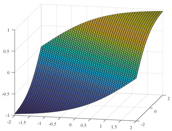
Figure 1.
3D structure diagram of S plane.
3.2. Fractional-Order Calculus
Fractional calculus is an extension of real calculus that can describe fractional-order calculus operations. Unlike integer-order calculus, the derivative and integral of fractional calculus can have any order. The future state of an integer-order dynamic system depends only on the current state (no memory). However, for fractional-order systems, the current state depends on the entire history of the system [28] (long-term memory). The main definitions of fractional calculus in modern control fields are Riemann–Liouville, Grunwald–Letnikov, and Caputo definitions [11].
For a function , its fractional-order Cauchy integral formula is:
where the order can be any positive real number, while the definition of a unified fractional calculus operator is:
In the equation, if and , the notation can be omitted. If the independent variable is t and there are no other variables, t can also be omitted. If , the operator represents the -th derivative of the function with respect to the independent variable t. represents the original signal, and if , it represents the -th integration.
The Grunwald–Letnikov fractional-order differentiation of the th order derivative of the function is defined as follows:
where, represents rounding to the nearest integer.
3.3. Fractional-Order Control
Traditional PID control model:
In the formula, , , and are three adjustable parameters.
The fractional-order controller has two additional parameters and compared to the traditional PID controller [29]. The transfer function of this controller is:
In Equation (16), the parameters that need to be adjusted are , , , as well as the orders and . In actual fractional-order controllers, due to the fact that the integral part is approximated by a filter, steady-state errors cannot be completely eliminated when , so it is necessary to reconstruct the integral part. The transfer function of the new fractional-order [29] controller is:
Perform the inverse Laplace transform on Equation (16) and combine S-plane control and FOPID control to obtain the actual control input formula
where
This article focuses on the quadrotor unmanned aerial vehicle, using a fractional-order S-shaped fusion control system. The specific control system is shown in Figure 2.
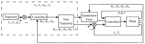
Figure 2.
Structure of quadrotor dual closed-loop control system.
In the control system shown in the figure above, represents the expected value of in the quaternion, while represents the quaternion obtained after model calculation. The error quaternion represents the difference between the measured attitude and the expected attitude, and can be expressed by the following equation:
4. Simulation and Result Analysis
4.1. Semi-Physical Simulation
As shown in the Figure 3, this article uses the hardware-in-the-loop simulation method to conduct trajectory-tracking experiments on a quadrotor unmanned aerial vehicle. The use of Raspberry Pi can provide powerful computing abilities for drones. The Ubuntu system it carries allows for users to freely modify the interface settings between the Raspberry Pi and the drone. By programming the Raspberry Pi, the control algorithm can be directly written into the ROS system. Through the Pixhawk, the quadcopter can be driven to fly along a predetermined trajectory, ultimately achieving the effect of trajectory tracking.
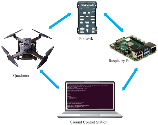
Figure 3.
Schematic diagram of hardware in the loop simulation system.
The main hardware equipment and their uses are introduced as follows:
- Host computer with a virtual machine of Ubuntu 22.04 and ROS system installed.
- Z410 drone, an experimental model designed for the entry-level development of drones.
- Pixhawk2.4.8 flight controller, necessary hardware for the normal flight of the drone, controlling the attitude of the drone.
- Raspberry Pi 4B, running external control programs and other system integrations, sending external control commands or network signals to the flight controller.
- Electronic speed controller (ESC), receiving the output signal of the flight controller, processing it and driving the motor to rotate.
- T-motor 2216 motor, where the motor rotation drives the propeller blades, providing upward power to the drone.
- Battery, the power source of the drone.
- Current meter, a component that supplies a dependable power source to the flight controller while detecting real-time voltage levels. It also takes preset actions for autonomous landing or return when the battery voltage is too low.
- UBEC, providing stable power supply to the Raspberry Pi.
- Receiver: paired with the remote controller, this receives the control signal from the remote controller to control the flight of the drone.
4.2. Matlab Simulation
To verify the effectiveness of the proposed method in this article, trajectory-tracking control simulation experiments were conducted based on a spiral trajectory. The experimental conditions were as follows: SIMULINK (MATLAB 2021a); the initial point of the drone was set to [0,0,0], i.e., the initial state was zero; and the simulation time was set to 40 s. The reference trajectory was given as follows:
4.3. Results Analysis
The parameters of the quadcopter can be initialized as follows:
In Table 1, we present the essential symbols, along with their corresponding parameters, which are referred to later in the document. Researchers injected white noise into the system attitude control input and position control input from 15–20 s in SIMULINK. The overall simulation results are shown in Figure 4:

Table 1.
Parameters and initial conditions.
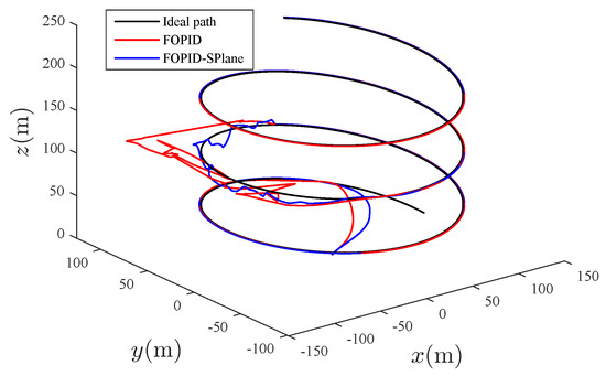
Figure 4.
Spiral trajectory-tracking plot.
The trajectory-tracking results of the quadcopter in the x, y, and z directions are shown in Figure 5, Figure 6, Figure 7, Figure 8, Figure 9, Figure 10, Figure 11, Figure 12 and Figure 13.
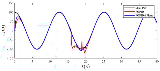
Figure 5.
Tracking effect in the x direction.
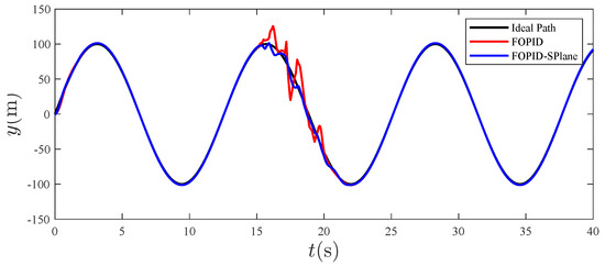
Figure 6.
Tracking effect in the y direction.
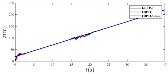
Figure 7.
Tracking effect in the z direction.
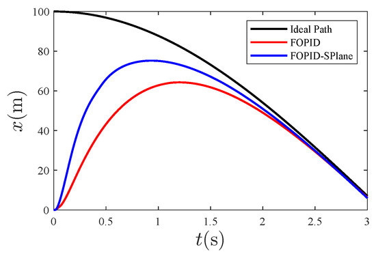
Figure 8.
Initial tracking in the x direction.
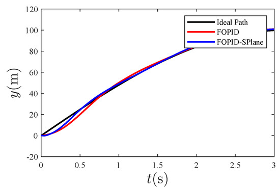
Figure 9.
Initial tracking in the y direction.
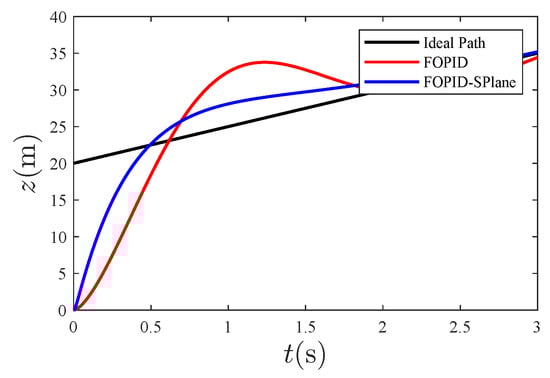
Figure 10.
Initial tracking in the z direction.
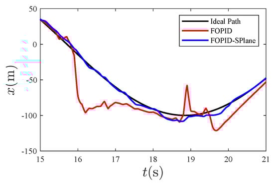
Figure 11.
Anti-disturbance effect in the x direction.
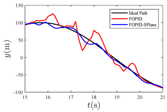
Figure 12.
Anti-disturbance effect in the y direction.
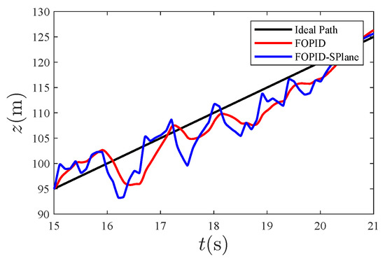
Figure 13.
Anti-disturbance effect in the z direction.
From Figure 7, it can be seen that the overall tracking effect of the designed controller is good. Zooming in on the tracking effect of 0∼3 s in the above figure, the following graph is obtained:
Enlarging the perturbation part in Figure 4, the resulting graph is as follows:
The expected path can be subtracted from the tracked trajectory results to obtain the error graphs for each direction as follows:
This article uses Equation (22) to quantitatively calculate the overall anti-interference quality of the fractional-order S-plane controller:
where represents the accumulated tracking error in the i direction. The calculation results are shown in the following table:
From Table 2, it can be seen that the fractional-order S-surface control is significantly smaller than the fractional-order PID control for tracking cumulative error, which is approximately of the fractional order PID.
Table 2.
Comparison of anti-interference quality between FOPID and FOPID-Splane control.
From Figure 4, it can be seen that, compared to traditional PID control, the fractional-order S-plane control not only quickly tracks the expected path with high precision, but also has the advantage of a high tracking accuracy. Figure 5, Figure 6 and Figure 7 show that the tracking effect of fractional-order S-plane control is significantly better than that of fractional-order PID control at the initial stage. When external wind disturbance is introduced from 15–20 s, the trajectory-tracking diagram of each coordinate axis and the trajectory-tracking error diagram of each coordinate axis in Figure 11, Figure 12, Figure 13, Figure 14, Figure 15 and Figure 16 that the fractional-order S-plane control designed in this paper has an excellent performance in terms of resisting wind disturbance.
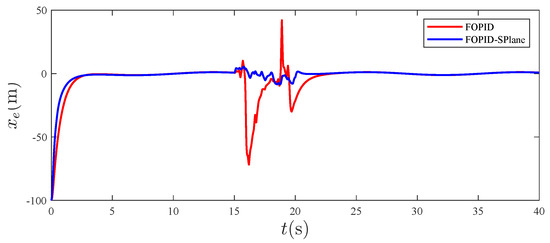
Figure 14.
Tracking error in the x direction.
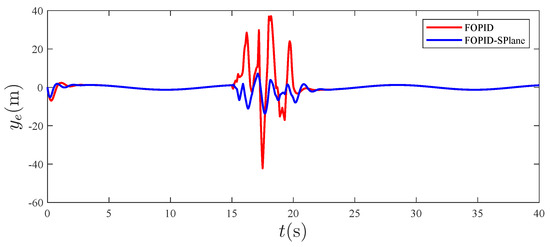
Figure 15.
Tracking error in the y direction.
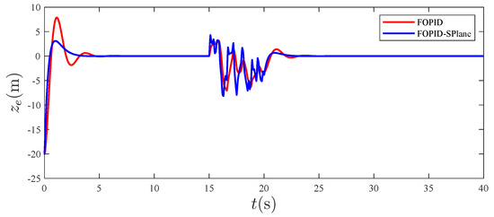
Figure 16.
Tracking error in the z direction.
5. Conclusions
5.1. Overall Summary
This article proposes a quaternion-based fractional-order S-surface fusion control strategy for the trajectory-tracking of quadrotor unmanned aerial vehicles. Simulation experiments were conducted using Matlab SIMULINK, and the following conclusions were drawn:
- The quaternion-based control model can effectively avoid singularity problems and facilitate the calculation of attitude angles.
- The designed fractional-order S-surface controller inherits the advantages of conventional PID controllers and can finetune the control system order to make the control process smoother.
- The simulation results show that, compared with fractional-order PID control, the fractional-order S-surface controller can give the control system a higher control accuracy and stronger robustness.
5.2. Further Research
Future research should consider the challenges of analysing the designed control system using math tools. Researchers resort to numerical methods to solve these equations because of their complexity, which can be time-consuming and computationally expensive. Fractional-order calculus is not as well-known as traditional integer calculus and requires a different approach to solve problems. The lack of familiarity with non-integer calculus makes it difficult for researchers to apply it to real-world problems, which often involve complex equations that are difficult to solve analytically. Therefore, mathematical analysis should be considered to verify the stability of the designed control system in future studies. For example, we will study the linearization of a nonlinear system to simplify the equations. An analysis of Lyapunov stability will be discussed in future work.
Author Contributions
Conceptualization, P.C.; methodology, J.L.; software, Z.C.; validation, L.G. and C.Z.; formal analysis, G.Z. and J.L.; investigation, Z.C. and G.Z.; resources, J.L.; data curation, C.Z.; writing—original draft preparation, Z.C.; writing—review and editing, J.L.; visualization, L.G.; supervision, P.C.; project administration, P.C.; funding acquisition, P.C. All authors have read and agreed to the published version of the manuscript.
Funding
This research was funded by the Key Research and Development Program of Shanxi Province (202202020101001), the National Natural Science Foundation of China (51909245, 62003314, 51279221), the Fundamental Research Program of Shanxi Province (202103021224187, 20210302124010, 20210302123050), and the Postgraduate Science and Technology Project of NUC (20221876).
Data Availability Statement
Not applicable.
Conflicts of Interest
The authors declare no conflict of interest. The funders had no role in the design of the study; in the collection, analyses, or interpretation of data; in the writing of the manuscript; or in the decision to publish the results.
Abbreviations
The following abbreviations are used in this manuscript:
| FOPID | Fractional order PID |
| SPlane | Sigmoid Plane |
References
- Li, J.; Li, Y. Dynamic analysis and PID control for a quadrotor. In Proceedings of the 2011 IEEE International Conference on Mechatronics and Automation, Beijing, China, 7–10 August 2011; pp. 573–578, ISSN 2152-744X. [Google Scholar] [CrossRef]
- Timis, D.D.; Muresan, C.I.; Dulf, E.H. Design and Experimental Results of an Adaptive Fractional-Order Controller for a Quadrotor. Fractal Fract. 2022, 6, 204. [Google Scholar] [CrossRef]
- Shi, X.; Cheng, Y.; Yin, C.; Dadras, S.; Huang, X. Design of fractional-order backstepping sliding mode control for quadrotor UAV. Asian J. Control 2019, 21, 156–171. [Google Scholar] [CrossRef]
- Han, J. Active Disturbance Rejection Control Technique—The Technique for Estimating and Compensating the Uncertainties; National Defense Industry Press: Beijing, China, 2008. [Google Scholar]
- Wang, C.; Chen, Z.; Sun, Q.; Zhang, Q. Design of PID and ADRC based quadrotor helicopter control system. In Proceedings of the 2016 Chinese Control and Decision Conference (CCDC), Yinchuan, China, 28–30 May 2016; pp. 5860–5865, ISSN 1948-9447. [Google Scholar] [CrossRef]
- Xu, R.; Ozguner, U. Sliding Mode Control of a Quadrotor Helicopter. In Proceedings of the 45th IEEE Conference on Decision and Control, San Diego, CA, USA, 13–15 December 2006; pp. 4957–4962, ISSN 0191-2216. [Google Scholar] [CrossRef]
- Shi, L.; Shen, J.; Wang, Q.; Jiang, J. Fuzzy Active Disturbance Rejection Attitude Control of Quadrotor Aircraft. Electr. Autom. 2021, 50, 157–162. [Google Scholar] [CrossRef]
- Muro, C.; Castillo-Toledo, B.; Loukianov, A.; Luque-Vega, L.; González-Jiménez, L. Quaternion-based trajectory tracking robust control for a quadrotor. In Proceedings of the 10th System of Systems and Engineering Conference, San Antonio, TX, USA, 17–20 May 2015; pp. 386–391. [Google Scholar] [CrossRef]
- Cheng, P.; Zhang, P.; Zhao, X.; Chang, J.; Yuan, M.; Shen, T. Expert S-Plane Control Method for Unmanned Aerial Vehicle. Aerosp. Control 2018, 36, 65–71. [Google Scholar] [CrossRef]
- Mandić, P.; Lazarević, M.; Šekara, T. D-decomposition technique for stabilization of Furuta pendulum: Fractional approach. Bull. Pol. Acad. Sci. Tech. Sci. 2016, 64, 189–196. [Google Scholar] [CrossRef]
- Liu, T. Fractional Order PID Control For a Quadrotor UAV. Master’s Thesis, Wuhan University of Science and Technology, Wuhan, China, 2021. [Google Scholar]
- Harrison, J.V.; Gallagher, J.L.; Grace, E.J. An algorithm providing all-attitude capability for three-gimballed inertial systems. IEEE Trans. Aerosp. Electron. Syst. 1971, AES-7, 532–543. [Google Scholar] [CrossRef]
- Liu, K.; Wang, R. Antisaturation Adaptive Fixed-Time Sliding Mode Controller Design to Achieve Faster Convergence Rate and Its Application. IEEE Trans. Circuits Syst. II Express Briefs 2022, 69, 3555–3559. [Google Scholar] [CrossRef]
- Islam, M.; Okasha, M. A Comparative Study of PD, LQR and MPC on Quadrotor Using Quaternion Approach. In Proceedings of the 7th International Conference on Mechatronics Engineering, Putrajaya, Malaysia, 30–31 October 2019; pp. 1–6. [Google Scholar] [CrossRef]
- Luukkonen, T. Modelling and control of quadcopter. Indep. Res. Proj. Appl. Math. Espoo 2011, 22. [Google Scholar]
- Zhou, Z.; Zhang, Q.; Liu, Q.; Zeng, Q.; Tian, X. Adaptive quaternion particle filter using generalized likelihood ratio test for aircraft attitude estimation in the presence of anomalous measurement. Meas. Sci. Technol. 2021, 32, 045004. [Google Scholar] [CrossRef]
- Figueredo, L.F.C.; Adorno, B.V.; Ishihara, J.Y.; Borges, G.A. Robust kinematic control of manipulator robots using dual quaternion representation. In Proceedings of the 2013 IEEE International Conference on Robotics and Automation, Karlsruhe, Germany, 6–10 May 2013; pp. 1949–1955. [Google Scholar]
- Antonelli, G.; Chiaverini, S.; Sarkar, N.; West, M. Adaptive control of an autonomous underwater vehicle: Experimental results on ODIN. IEEE Trans. Control Syst. Technol. 2001, 9, 756–765. [Google Scholar] [CrossRef]
- Voight, J. Quaternion Algebras; Springer International Publishing: Berlin/Heidelberg, Germany, 2021. [Google Scholar]
- Quan, Q. Introduction to Multicopter Design and Control; Springer: Singapore, 2018. [Google Scholar]
- Cariño, J.; Abaunza, H.; Castillo, P. Quadrotor quaternion control. In Proceedings of the 2015 International Conference on Unmanned Aircraft Systems (ICUAS), Denver, CO, USA, 9–12 June 2015; pp. 825–831. [Google Scholar] [CrossRef]
- Hu, S. Design of Control Method for Nonlinear Underactuated Quadrotor Aircraft; National Defense Industry Press: Beijing, China, 2021. [Google Scholar]
- Liu, K.; Wang, R.; Wang, X.; Wang, X. Anti-saturation adaptive finite-time neural network based fault-tolerant tracking control for a quadrotor UAV with external disturbances. Aerosp. Sci. Technol. 2021, 115, 106790. [Google Scholar] [CrossRef]
- Liu, K.; Wang, R.; Zheng, S.; Dong, S.; Sun, G. Fixed-time disturbance observer-based robust fault-tolerant tracking control for uncertain quadrotor UAV subject to input delay. Nonlinear Dyn. 2022, 107, 2363–2390. [Google Scholar] [CrossRef]
- Wu, G.; Luo, W.; Guo, J.; Zhang, J. A Sigmoid-plane adaptive control algorithm for unmanned surface vessel considering marine environment interference. Trans. Inst. Meas. Control 2022, 44, 2076–2090. [Google Scholar] [CrossRef]
- Li, Y.; Pang, Y.; Wan, L. Adaptive S Plane Control for Autonomous Underwater Vehicle. J. Shanghai Jiaotong Univ. 2012, 46, 195–200+206. [Google Scholar] [CrossRef]
- Chen, P.; Zhang, G.; Guan, T.; Yuan, M.; Shen, J. The Motion Controller Based on Neural Network S-Plane Model for Fixed-Wing UAVs. IEEE Access 2021, 9, 93927–93936. [Google Scholar] [CrossRef]
- Monje, C.A.; Chen, Y.; Vinagre, B.M.; Xue, D.; Feliu-Batlle, V. Fractional-Order Systems and Controls: Fundamentals and Applications; Springer Science & Business Media: Berlin/Heidelberg, Germany, 2010. [Google Scholar]
- Podlubny, I. Fractional-order systems and PIλDμ-controllers. IEEE Trans. Autom. Control 1999, 44, 208–214. [Google Scholar] [CrossRef]


Disclaimer/Publisher’s Note: The statements, opinions and data contained in all publications are solely those of the individual author(s) and contributor(s) and not of MDPI and/or the editor(s). MDPI and/or the editor(s) disclaim responsibility for any injury to people or property resulting from any ideas, methods, instructions or products referred to in the content. |
© 2023 by the authors. Licensee MDPI, Basel, Switzerland. This article is an open access article distributed under the terms and conditions of the Creative Commons Attribution (CC BY) license (https://creativecommons.org/licenses/by/4.0/).