Enhanced Tyre Pressure Monitoring System for Nitrogen Filled Tyres Using Deep Learning

Abstract

Tyre pressure monitoring systems (TPMS) are electronic devices that monitor tyre pressure in vehicles. Existing systems rely on wheel speed sensors or pressure sensors. They rely on batteries and radio transmitters, which add to the expense and complexity. There are two types of basic tyres: non-pneumatic and pneumatic tyres. Non-pneumatic tyres lack air and combine the tyre and wheel into a single unit. When it comes to noise reduction, durability, and shock absorption, pneumatic tyres are more valuable than non-pneumatic tyres. In this study, nitrogen-filled pneumatic tyres were considered due to the uniform pressure management property. Additionally, nitrogen has less of an effect on thermal expansion than regular air-filled tyres. This work aimed to offer a deep learning approach for TPMS. An accelerometer captured vertical vibrations from a moving vehicle’s wheel hub, which were then converted in the form of vibration plots and categorized using pretrained networks. The most popular pretrained networks such as AlexNet, GoogLeNet, ResNet-50 and VGG-16 were employed in this study. From these pretrained networks, the best-performing pretrained network was determined and suggested for TPMS by varying the hyperparameters such as learning rate (LR), batch size (BS), train-test split ratio (TR), and solver (SR). Findings: A higher classification accuracy of 97.20% was obtained while using ResNet-50.

1. Introduction

The circular-shaped components that surround the rims of automobiles to strengthen the axial load are called tyres. There are two types of basic tyres—non-pneumatic and pneumatic. The majority of passenger car and bicycle tyres are air-inflated structures. As they roll, these tyres provide the passenger with a flexible cushion effect by absorbing vertical vibrations. Non-pneumatic tyres lack air and combine the tyre and wheel into a single unit. These tyres are found in specialized vehicles such as riding lawnmowers and tractors. When it comes to noise reduction, durability, and shock absorption, pneumatic tyres are more valuable than non-pneumatic tyres [1]. Pneumatic tyres are classified as bias-ply, radial-ply, or belted-ply, depending on how they are made. Nowadays, nitrogen-filled tyres in cars are common as they have the ability to keep constant tyre pressure [2]. Nitrogen has a lesser impact on thermal expansion when compared to ordinary air-filled tyres; it also acts as a cooling agent to the tyres when they are used for long distance travel and it also reduces fuel consumption due to the decrease in vibration velocity [3]. One of the primary advantages of using nitrogen to fill tyres is its ability to sustain tyre pressure consistently over time. Nitrogen molecules are larger and less permeable than oxygen molecules, which are commonly found in air-filled tyres, resulting in slower pressure loss. 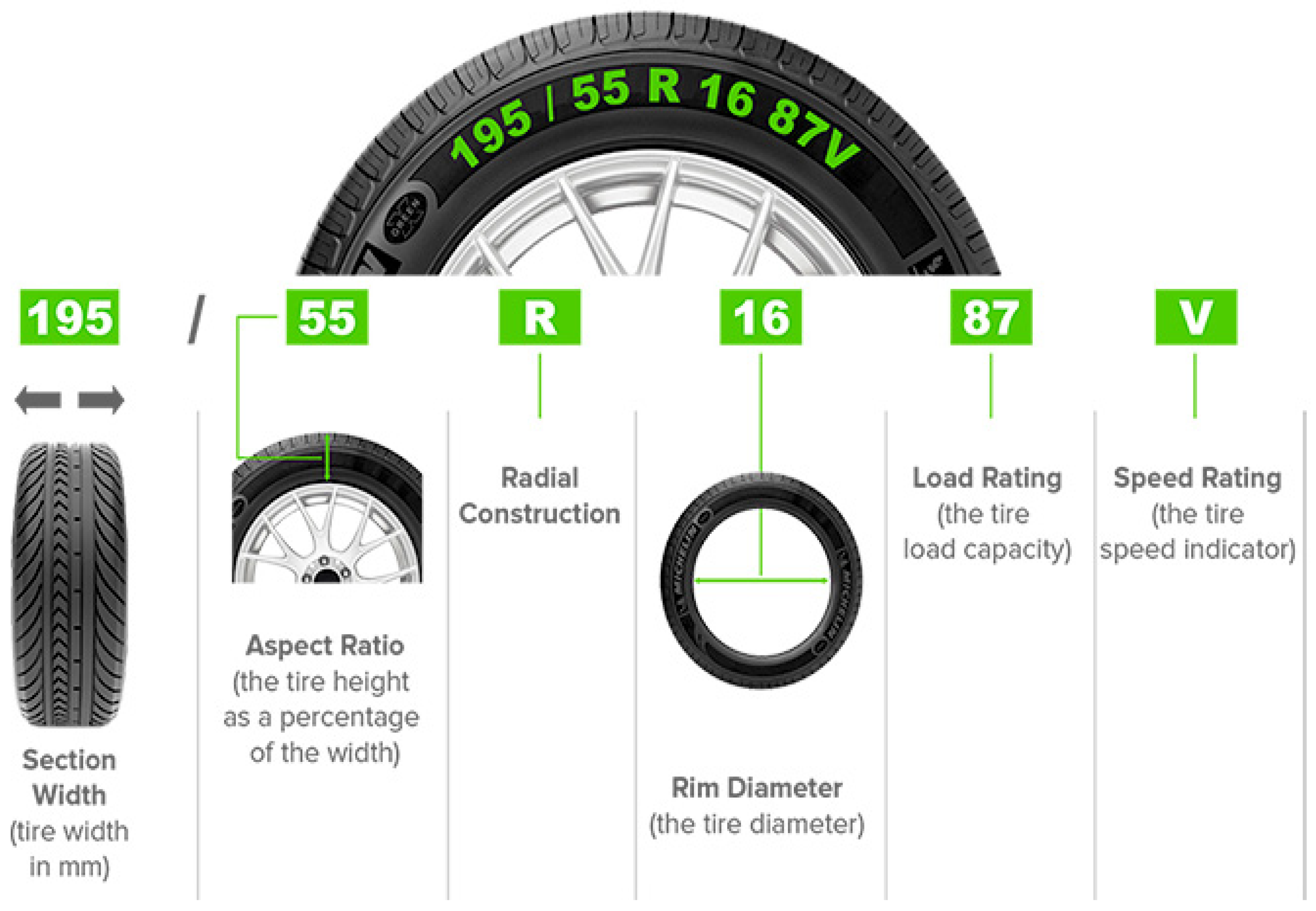This feature can help to keep tyre pressure at the appropriate level, resulting in increased rolling resistance and improved fuel efficiency [4,5]. In this study, we considered pneumatic tyres filled with nitrogen air. The tyre utilized in this research was labelled 145/70 R12 69 T. The tyre width is 145 mm, the construction type is radial, and 70% of the width is taken up by the side wall. The radial structure is represented by the letter ‘R’. The tyre requires a rim size of 12 inches. The load index value is ‘69’; the maximum allowed load is reflected by it. In this situation, ‘69’ is 325 kg. The speed rating code ‘T’ indicates the tyre’s maximum safe speed. In this example, ‘T’ = 190 km/h. Figure 1 displays a sample of a radial tyre; it contributes to comfort and fuel efficiency, and therefore it is frequently utilized in automobiles.

TPMS are vehicle electronic devices that monitor tyre pressure. The TPMS can track each individual tyre’s pressure and display tyre pressure data to the driver. Direct TPMS (DTPMS) systems measure air pressure within the tyre using barometric pressure sensors, whereas indirect methods depend on external characteristics such as wheel radius. According to the manufacturer’s recommendations, excellent handling and fuel economy are achieved by inflating the tyre. DTPMS rely on temperature sensors and barometric pressure, which are integrated. Indirect TPMS (ITPMS) indirectly measures pressure and tyre condition using wheel speed sensors and data are sent to the controlling unit.

The benefits of ITPMS include low costs, dependability and ease of maintenance. IT-PMS research prospects in current emerging technologies such as deep learning, artificial intelligence, machine learning, and so on, have gained widespread recognition in recent years [6].

(a)

Deep Learning-based ITPMS: Deep learning algorithms have been shown to be effective at detecting anomalies and predicting failures in various systems, including ITPMS. Researchers have developed deep learning-based ITPMS that can accurately predict tyre pressure deviations and alert the driver when the pressure drops below the recommended level. Overall, the study demonstrates the potential of using machine learning and simulation tools to develop indirect tyre-pressure monitoring systems, which can provide a cost-effective and efficient solution for monitoring tyre pressure in vehicles [7].

(b)

Machine Learning-based ITPMS: Machine learning algorithms have been applied to ITPMS to analyse tyre pressure data and identify patterns that can indicate potential tyre failures. Machine learning-based ITPMS can predict tyre failures with high accuracy and provide early warning to drivers, helping them to avoid accidents. Overall, the study provides valuable insights into the development of an indirect TPMS using machine learning techniques. It demonstrates the potential of ML in accurately predicting tyre pressure and lays out a methodology for developing such systems. The study has important implications for ride comfort, safety, and optimum vehicle handling performance, and has the potential to contribute to the development of more efficient and cost-effective TPMS solutions [8].

(c)

Intelligent tyre management: AI-powered tyre management systems can use data from ITPMS sensors to optimize tyre performance and longevity. For example, they can recommend tyre rotations and pressure adjustments based on driving conditions and usage patterns. Overall, the study provides an overview of the current state of TPMS and presents a self-designed TPMS system that can effectively monitor tyre pressure and ensure safety while driving [9].

(d)

Real-time monitoring: Advanced analytics and AI can be used to process data from ITPMS sensors in real-time, providing drivers with up-to-date information on their tyre pressure and temperature. This can help prevent accidents and improve fuel efficiency. Overall, the study demonstrates the potential of using an ANN-based method for tyre pressure monitoring, which can simplify the data pre-processing and improve the response speed and working range of the system. This can ultimately enhance driving safety and reduce the risk of accidents caused by deflated tyres [10].

1.1. Related Works

This section outlines the existing research studies and experiments related to TPMS, including those that have addressed the limitations of early TPMS systems. Some of these studies have employed sophisticated signal processing and spectrum analysis methods to detect underinflated tyres, while others have focused on monitoring wheel balance and tyre pressure through frequency spectrum analysis and vibration measurements of the tyre. The biggest disadvantage of this technology is that it does not detect when all four tyres are underinflated at the same time. Later investigations, however, corrected this flaw using sophisticated signal processing and spectrum analysis methods. According to Schuring et al. [11] the increase in fuel efficiency caused by tyre stiffness occurs when the rolling resistance coefficient decreases. Robinson et al. [12] set up an experiment in which a tyre was struck with a hammer to create vibrations while an accelerometer was mounted to the tyre. In a separate study, Craighead et al. [13] recommended employing frequency spectrum analysis and vibration measurements of the tyre under typical operating conditions to determine wheel balance and tyre pressure. The accuracy of the imbalance measure that was created was less than 12%. Tyre lifespan is proportional to tyre pressure. A 1% change in tyre pressure can increase total fuel consumption by 2% and reduce tyre life by 25%. Chandolikar et al. [14] suggested several energy harvesting strategies utilizing TPMS and came to the conclusion that piezoelectric sensors are important in TPMS. Some of the technologies that are only used in commercial vehicles use the Vehicle Stability Sensor and GPS to measure tyre pressure and radius [15]. Fuzzy logic was applied to a strain-based technique by Garcia-Pozuelo et al. to track rolling speed, vertical load, and inflation pressure [16].

The investigations based on the ITPMS method must acquire traction. Svensson et al. [17] presented an ITPMS using supervised machine learning. In general, numerous noteworthy experiments in the fields of DTPMS and ITPMS were carried out. However, just a few experiments have been conducted to detect both tyre balance and tyre pressure using ITPMS. Furthermore, adequate attention should be placed on trials based on machine learning. Anoop et al. have proposed various machine learning algorithms for a tyre pressure monitoring system, which require a deeper understanding of feature engineering [18,19,20].

1.2. Research Gap

The major disadvantage of TPMS technology is that it does not detect when all four tyres are underinflated at the same time. While later investigations have corrected this flaw using advanced signal processing and spectrum analysis methods, only a few experiments have been conducted to detect both tyre balance and tyre pressure using indirect TPMS and machine learning approaches. Therefore, there is a research gap in developing a comprehensive TPMS system that can accurately detect both tyre balance and tyre pressure using indirect TPMS and machine learning approaches.

1.3. Technical Contribution

This work proposes a unique strategy for developing a TPMS. This system can detect both tyre balance and tyre pressure using indirect methods and deep learning approaches. To achieve this, the proposed system uses vibration signals acquired from an accelerometer as input. The deep learning model is trained on a dataset consisting of vibration signals and corresponding tyre pressure and balance values. The developed system is expected to provide an accurate and reliable solution for monitoring tyre pressure and balance in vehicles. CNN are the core building blocks of deep learning that are used to extract detailed information from visual input. CNN is frequently utilized as one of the most successful methods for object identification, speech recognition and defect detection.

Table 1. Several studies on DL-based techniques for mechanical systems.

Reference	Deep Learning Technique	Mechanical System
[25]	CNN with wavelet transformation	Motor Bearing
[26]	CNN	Roller Bearing
[27]	Hierarchical CNN
[28]	CNN	Centrifugal pump
[29]	Stacked auto encoder
[30]	Recurrent neural network	Gear box
[31]	Deep belief network and sparse auto encoder
[32]	Generative adversarial network
[33]	SVM	Cutting tool
[34]	Principle Component Analysis and DT
[35]	ANNBFIS, Free Forward Back Propagation and Free Forward Back Propagation Neural Network
[36]	Deep learning

lists numerous significant articles that demonstrate the usage of CNN in automated systems. In this work, TPMS was carried out utilizing well-known and entrenched pretrained deep learning models such as ResNet-50 [21], GoogLeNet [22], VGG-16 [23] and AlexNet [24]. The network models described above are referred to as “pretrained”, since they were trained using a variety of existing datasets including a diverse collection of classes and objects. As a result of their training, these pretrained networks have past knowledge that can be transferred and utilized to address specific issues (transfer of knowledge to a different domain). Transfer learning refers to the process of transferring knowledge. Algorithmic advancements in recent years have increased the level of categorization accuracy to a greater extent. In this study, the efficacy of several pretrained networks was examined to determine tyre condition using images produced from vibration signals. Experiments on pretrained networks were carried out by modifying several hyperparameters such as the train–test split ratio (TR), solver (SR), batch size (BS) and learning rate (LR). The results were analysed and summarized in order to establish the optimal network for TPMS.

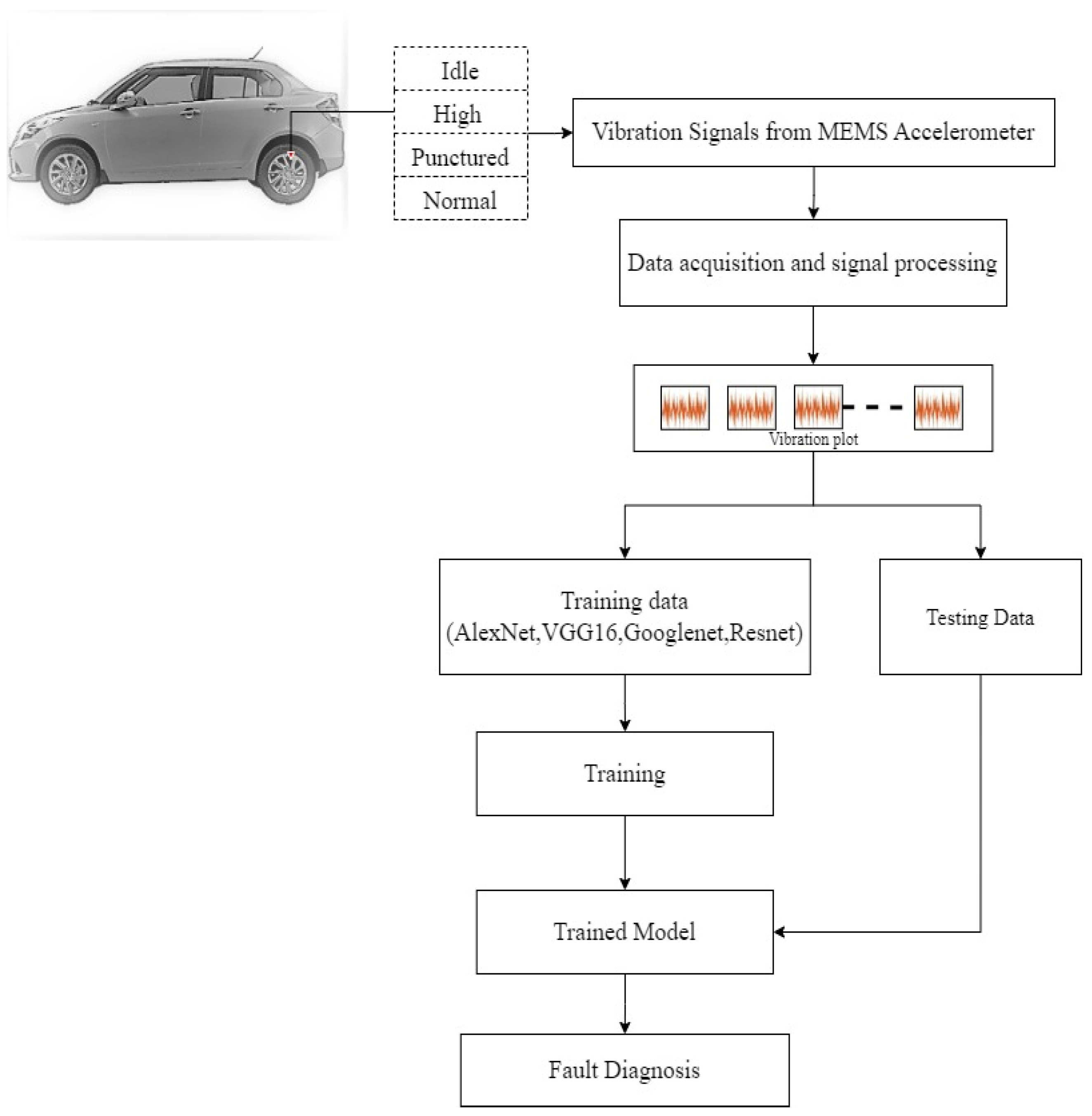
The technical contribution of this effort is highlighted by the analysis of four tyre conditions, namely high pressure, puncture, idle, and normal. To achieve this, signals received from a sensor were collected and plotted as images. These images were then used as inputs for pretrained networks such as ResNet-50, GoogLeNet, VGG-16, and AlexNet, which were utilized in TPMS testing for a vehicle. By adjusting key parameters such as LR, SR, BS, and TR, the accuracy of the pretrained networks was examined, and the optimal network for TPMS was identified based on the results obtained. The overall workflow of the methodology is presented in Figure 2.

2. Experimental Procedures

This section describes in detail the experimental setup and the technique used to perform tyre condition monitoring with pretrained neural networks.

2.1. Experimental Setup

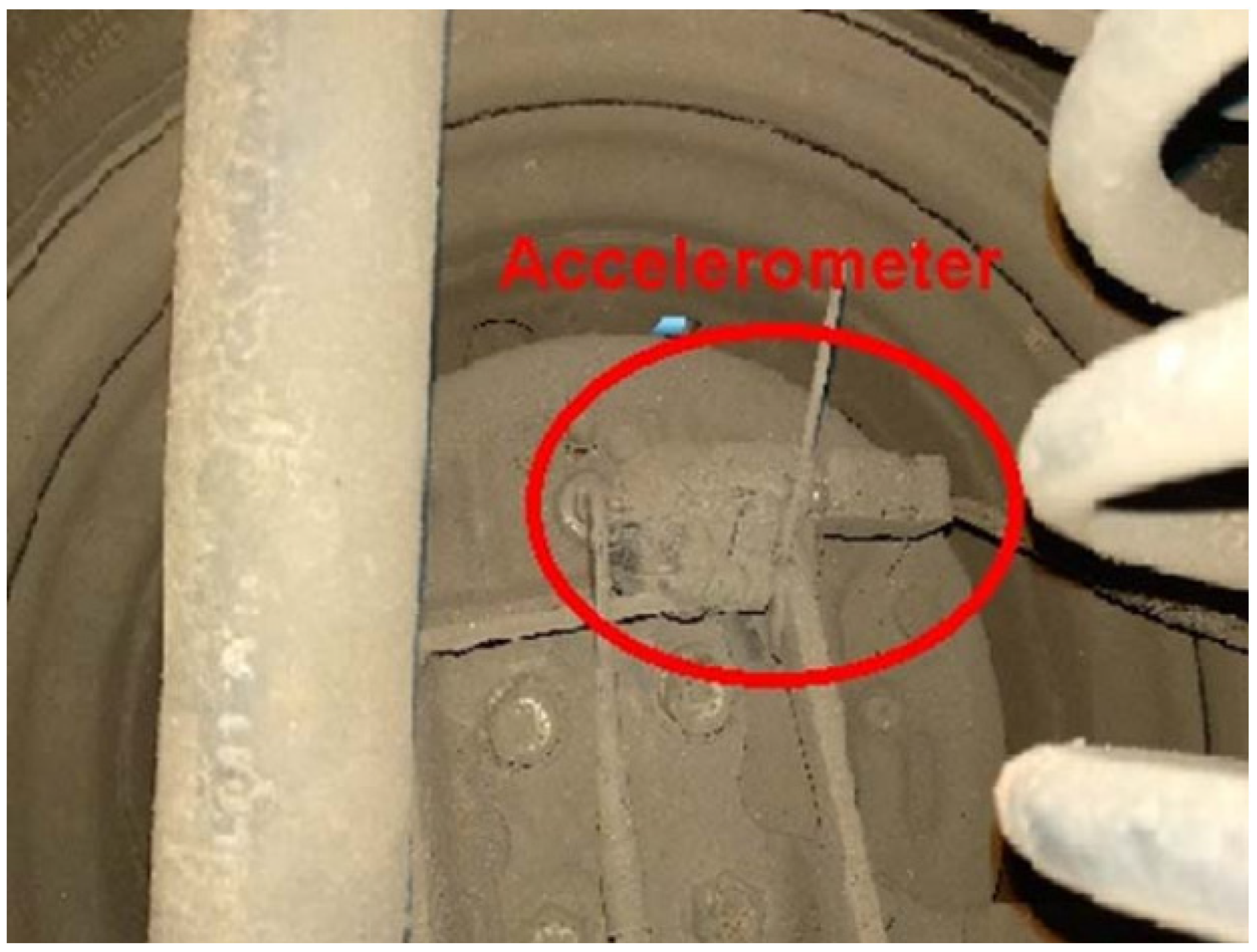
To conduct the experiment, a vehicle with front-wheel drive was chosen and vertical vibration signals were obtained from the rear left wheel axis, which had a nitrogen-filled pneumatic tyre. A waterproof tri-axial MEMS accelerometer (MMA7361L) with a resonant frequency of 6 kHz, a frequency range of 1 to 400 Hz, and a sensitivity of 206 mV/g was applied to the rear left wheel hub. The accelerometer was oriented to measure vertical vibrations along the Y axis, which was the main focus of the study. The experiment was not carried out on a static test rig inside a laboratory. In order to make the study as realistic as possible, the vehicle (car) was driven on a national highway in India (the road condition is reasonably good) and the signals were acquired. The sensor was mounted on the top surface of the axle (that is not rotating) using an adhesive mounting technique. The sensor cables were then taken to the front seat and connected to the DAQ cord which in turn was connected to a laptop for data acquisition. Figure 3 depicts the specific MEMS accelerometer that was utilized to gather vibration data for this investigation.

2.2. Data Acquisition

To enable digital signal processing and signal conditioning, an appropriate data acquisition device (DAQ) was utilized to collect and convert analogue signals from the accelerometer. For this study, the NI USB-6001 was selected, as it provides 12 input channels, a 14-bit resolution, and a maximum sampling rate of 20 kS/s. The NI LabVIEW software 2013 interface was utilized to establish a connection between the DAQ output and the computer system. The accelerometer’s analogue vibrations were captured and converted into digital signals by the DAQ system, with a shield wire employed to minimize the effects of external electronic interference. Finally, the DAQ output was connected to the monitoring computer system through the NI LabVIEW software interface.

2.3. Experimental Procedure

This study focused on the analysis of a tyre that was in a balanced condition, meaning no additional weight was added beyond the existing balancing weight (40 g). Data were collected for various pressure conditions, including High, Normal, Punctured, and Idle.

• For the Normal condition, a tyre pressure of 31 psi was selected based on the manufacturer’s specifications, and experiments were conducted at speeds ranging from 10 km/h to 100 km/h within the legal speed limits on National Highway India;
• For the High pressure condition, a tyre pressure of 40 psi was selected, and signals were collected with the help of a tri-axial MEMS accelerometer at speeds ranging from 10 km/h to 100 km/h on National Highway India;
• The Punctured condition was simulated with a tyre pressure of 19 psi for safety reasons, as selecting 0 psi could potentially cause an accident. The proposed network was designed to alert the driver when the tyre pressure reaches 19 psi to indicate a puncture;
• For the Idle condition, vibration signals were taken at a speed of 10 km/h because the signals collected for the Normal condition could potentially be misclassified, as these signals were taken at speeds ranging from 10 km/h to 100 km/h.

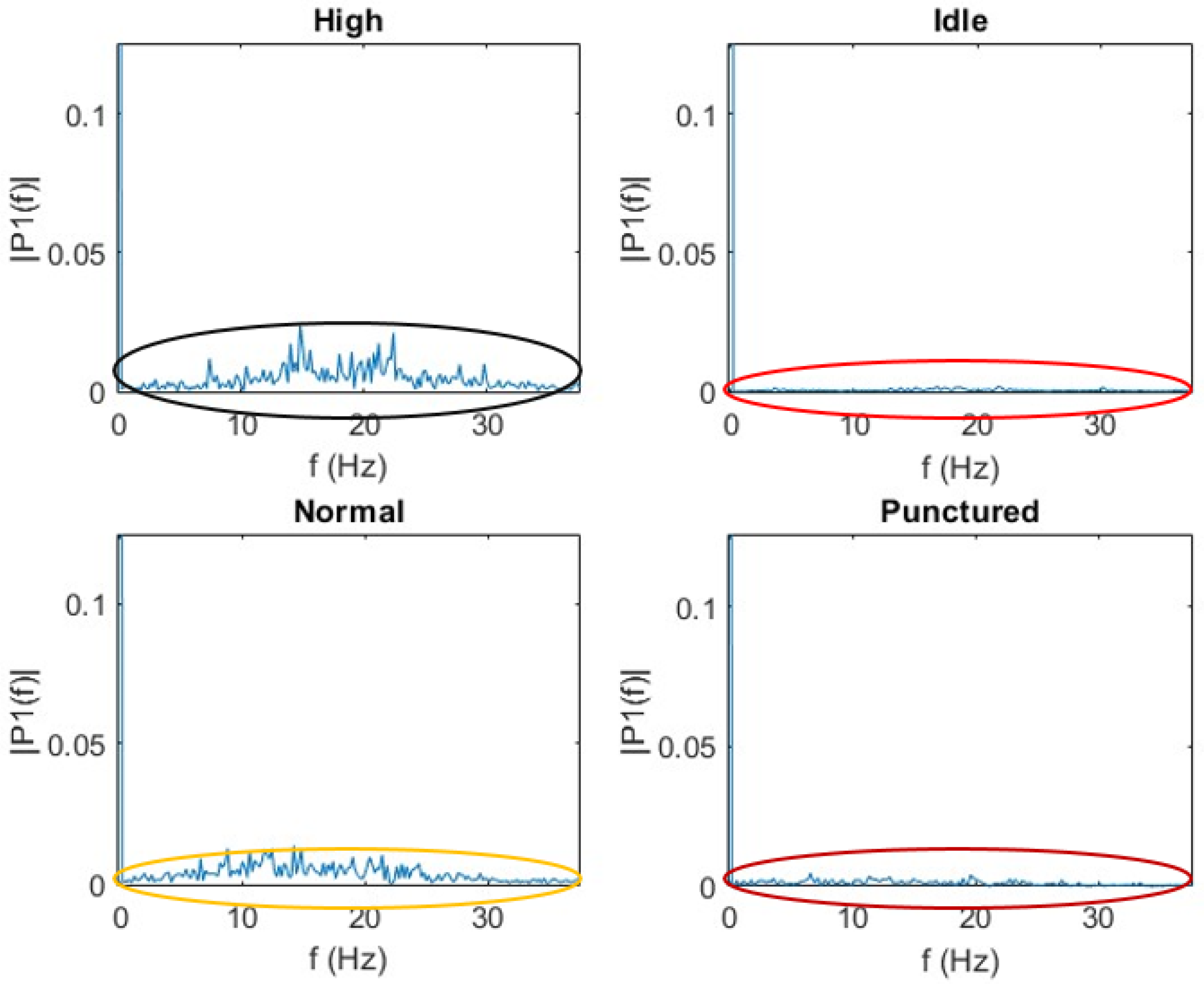
A total of 240 signals were analysed, with 60 data points extracted for each signal and converted into corresponding vibration plots. In total, 1200 samples were collected under various balance circumstances, with a sampling frequency of 1 kHz and 5000 data points per sample. Figure 4 represents the vibration signals of different conditions used, where the x-axis represents the sample number and the y-axis represents the amplitude. The Fast Fourier Transform (FFT) is a handy technique for analysing the frequency content of a signal. Figure 5 shows the variances between the four classes of signals after obtaining the FFT of the data.

3. Convolution Neural Networks (CNNs)

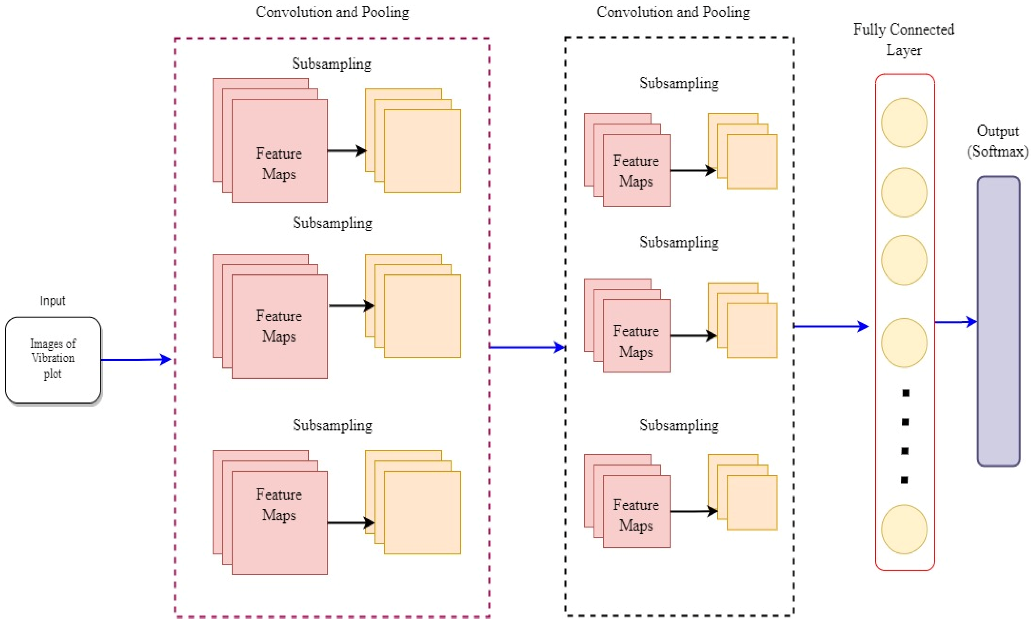
CNN uses a set of weights and biases to create a relationship between image attributes and visual representation through an automatic feature learning method. It uses a hierarchical design with three layers: convolution, pooling, and fully connected. The convolution layer takes input from the input layer, while the pooling layer performs down sampling. The fully connected layer produces classification results for specific issues (Figure 6). Fully connected layers use activation functions such as softmax and sigmoid. Pooling layers reduce the dimensionality of data and minimize computational complexity. Convolution layers use learnable kernels or filters and can optimize hyperparameters such as depth, stride, and zero-padding.

4. Pressure Monitoring of Tyre Using Pre-Trained Network

This study investigated the tyre condition—which is described in this section—using many pretrained networks. At first, vibration charts were created by recording vibration signals for different tyre settings (images). According to the input requirements of the chosen pretrained model, the obtained images were further scaled and pre-processed to a size of $227\times 227$ or $224\times 224$. A variety of well-known pretrained network models, including GoogLeNet, ResNet-50, VGG-16 and AlexNet, were also employed to undertake image classification and assess the status of the tyre. In this study, transfer learning was utilized to recover the original values of ImageNet networks. To meet the user-specified number of classes, a custom dataset was employed, and new layers were utilized to replace the final output layer. The whole TPMS process employed pretrained networks. The following is a short rundown of how the pretrained mode was used in this research. Figure 7 represents the overall workflow.

Creation and Pre-Processing of Datasets

The vibration data collected in this investigation were used to generate a set of photographs containing the tyre condition. In this investigation, four circumstances were considered: Normal, High, Puncture and Idle tyre conditions. The vibration signals acquired were used to generate 240 images, 60 for each class. The collected photos were downsized to $224\times 224$ or $227\times 227$ in order for the input size of the picture to be adequate for the pretrained network employed. The models used in this study are discussed below:

ResNet-50: The ResNet network, developed by He et al. for the annual ILSVRC 2015, proved to be the most successful and productive. High convergence rates and precise categorization were the main benefits of employing the ResNet architecture. The common objects in context (COCO) dataset served as the training ground for the ResNet architecture and it was created using the remaining units. Numerous ResNet topologies are possible due to the number of layers and residual units available. Identities being shortened, in which the identity of the output value is the same as the identity of the input value, is what allowed for the creation of the ResNet design. ResNet features fully linked layers with convolution pooling, much as other networks. ResNet and VGG networks have comparable architectures. However, because the latter is eight times deeper, it includes eight times as many learnable parameters. The ResNet-50 [21] architecture consists of one fully linked layer and 49 convolutional layers.

GoogLeNet: The architecture of GoogLeNet [22] consists of 22 layers and has various applications in robotics, adversarial training and facial recognition. The network is made up of nine inception modules that are coupled to four convolutions, four max pooling layers, three softmax layers, five fully connected layers and three average pooling layers. A ratio of 0.5 is utilized by the dropout layer to support the activation function used in entirely connected layers; this is referred to as ReLU. The GoogLeNet architecture inception modules enable the network to deal with progressively difficult computer vision problems. The main benefit of using inception modules is the ability to identify complicated characteristics through changes in convolution layer filter size. A technique such as this can help reduce computational complexity and time. The GoogLeNet architecture, although having 22 layers and a powerful look, has fewer trainable parameters than AlexNet.

AlexNet: The network is made up of 11 layers. The large number of layers in the network increases feature extraction. The picture input layer is a pre-processing layer in our deep learning system that reduces the input frame spatial resolution from $640\times 480$ to $227\times 227$ in order to reduce the computing cost of the system. Furthermore, the number of components has a negative influence on speed. The first layer of the AlexNet [24] is the convolution layer with dimensions of $227\times 227\times 3$ for height, width and depth, respectively. Following the convolution layer are the maximum pooling and normalising layers. The last layer is the softmax, which is in charge of categorization. The model is composed of five convolutional layers and three fully linked layers.

VGG-16: The 2014 ImageNet competition saw architectural innovations with considerable speed and extensive stacking. To accomplish efficient convolution, the VGG network was built with the goal of stacking deeper network layers with more compact filters. The title honours the Oxford University researchers who formed the Virtual Geometry Group (VGG). The VGG network comprises 16 or 19 layers and is far deeper than AlexNet. The VGG network extracts more unique features by distributing tiny filters ($3\times 3$) uniformly across all convolution layers. The network layers were all pooled on a regular basis, which simplified the network structure. The number of learnable parameters is decreased when smaller filter sizes are used, which lowers the convolution process dimensional and computational complexity. In the VGG design, deeper, smaller filters are employed rather than larger, memory-intensive filters. The functioning of 22 convolutional layers was recreated by the receptive field of the VGG architecture. In the VGG-16 [23] architecture, there are sixteen convolutional layers that are completely coupled.

5. Evaluation Metrics

Evaluation metrics play a crucial role in measuring the effectiveness of machine learning models by quantifying their performance in accomplishing the intended task. Several commonly used evaluation metrics, such as Area Under the Curve (AUC), sensitivity, specificity, and F1 score, are also commonly used in machine learning and statistical analysis to evaluate the performance of models.

• Area Under the Curve (AUC) is a metric commonly used in classification problems to measure the performance of a model predictions. It represents the area under the Receiver Operating Characteristic (ROC) curve, which is a plot of the true positive rate (sensitivity) against the false positive rate (1-specificity) for different threshold values. AUC ranges from 0 to 1, with higher values indicating better performance.

$$\mathbf{A}\mathbf{U}\mathbf{C}=\frac{\left(\mathbf{T}\mathbf{r}\mathbf{u}\mathbf{e} \mathbf{P}\mathbf{o}\mathbf{s}\mathbf{i}\mathbf{t}\mathbf{i}\mathbf{v}\mathbf{e}\times \mathbf{T}\mathbf{r}\mathbf{u}\mathbf{e} \mathbf{N}\mathbf{e}\mathbf{g}\mathbf{a}\mathbf{t}\mathbf{i}\mathbf{v}\mathbf{e}\right)-\left(\mathbf{F}\mathbf{a}\mathbf{l}\mathbf{s}\mathbf{e} \mathbf{P}\mathbf{o}\mathbf{s}\mathbf{i}\mathbf{t}\mathbf{i}\mathbf{v}\mathbf{e}\times \mathbf{F}\mathbf{a}\mathbf{l}\mathbf{s}\mathbf{e} \mathbf{N}\mathbf{e}\mathbf{g}\mathbf{a}\mathbf{t}\mathbf{i}\mathbf{v}\mathbf{e}\right)}{\left(\mathbf{T}\mathbf{r}\mathbf{u}\mathbf{e} \mathbf{P}\mathbf{o}\mathbf{s}\mathbf{i}\mathbf{t}\mathbf{i}\mathbf{v}\mathbf{e}+\mathbf{F}\mathbf{a}\mathbf{l}\mathbf{s}\mathbf{e} \mathbf{N}\mathbf{e}\mathbf{g}\mathbf{a}\mathbf{t}\mathbf{i}\mathbf{v}\mathbf{e}\right)\times \left(\mathbf{F}\mathbf{a}\mathbf{l}\mathbf{s}\mathbf{e} \mathbf{P}\mathbf{o}\mathbf{s}\mathbf{i}\mathbf{t}\mathbf{i}\mathbf{v}\mathbf{e}+\mathbf{T}\mathbf{r}\mathbf{u}\mathbf{e} \mathbf{N}\mathbf{e}\mathbf{g}\mathbf{a}\mathbf{t}\mathbf{i}\mathbf{v}\mathbf{e}\right)}.$$

• Specificity is also commonly used in classification problems and measures the proportion of true negatives (correctly classified negatives) out of all actual negatives. Specificity can be useful in situations where the costs of false positives and false negatives are different.

$$\mathbf{S}\mathbf{p}\mathbf{e}\mathbf{c}\mathbf{i}\mathbf{f}\mathbf{i}\mathbf{c}\mathbf{i}\mathbf{t}\mathbf{y}=\frac{\left(\mathbf{T}\mathbf{r}\mathbf{u}\mathbf{e} \mathbf{P}\mathbf{o}\mathbf{s}\mathbf{i}\mathbf{t}\mathbf{i}\mathbf{v}\mathbf{e}\right)}{\left(\mathbf{T}\mathbf{r}\mathbf{u}\mathbf{e} \mathbf{P}\mathbf{o}\mathbf{s}\mathbf{i}\mathbf{t}\mathbf{i}\mathbf{v}\mathbf{e}+\mathbf{F}\mathbf{a}\mathbf{l}\mathbf{s}\mathbf{e} \mathbf{N}\mathbf{e}\mathbf{g}\mathbf{a}\mathbf{t}\mathbf{i}\mathbf{v}\mathbf{e}\right)}.$$

• Precision measures the proportion of correctly classified positive instances out of the total number of instances predicted as positive. It is defined as follows:

$$\mathbf{P}\mathbf{r}\mathbf{e}\mathbf{c}\mathbf{i}\mathbf{s}\mathbf{i}\mathbf{o}\mathbf{n}=\frac{\left(\mathbf{T}\mathbf{r}\mathbf{u}\mathbf{e} \mathbf{P}\mathbf{o}\mathbf{s}\mathbf{i}\mathbf{t}\mathbf{i}\mathbf{v}\mathbf{e}\right)}{\left(\mathbf{T}\mathbf{r}\mathbf{u}\mathbf{e} \mathbf{P}\mathbf{o}\mathbf{s}\mathbf{i}\mathbf{t}\mathbf{i}\mathbf{v}\mathbf{e}+\mathbf{F}\mathbf{a}\mathbf{l}\mathbf{s}\mathbf{e} \mathbf{P}\mathbf{o}\mathbf{s}\mathbf{i}\mathbf{t}\mathbf{i}\mathbf{v}\mathbf{e}\right)}.$$

• Recall measures the proportion of correctly classified positive instances out of the total number of actual positive instances. It is defined as follows:

$$\mathbf{R}\mathbf{e}\mathbf{c}\mathbf{a}\mathbf{l}\mathbf{l}=\frac{\left(\mathbf{T}\mathbf{r}\mathbf{u}\mathbf{e} \mathbf{P}\mathbf{o}\mathbf{s}\mathbf{i}\mathbf{t}\mathbf{i}\mathbf{v}\mathbf{e}\right)}{\left(\mathbf{T}\mathbf{r}\mathbf{u}\mathbf{e} \mathbf{P}\mathbf{o}\mathbf{s}\mathbf{i}\mathbf{t}\mathbf{i}\mathbf{v}\mathbf{e}+\mathbf{F}\mathbf{a}\mathbf{l}\mathbf{s}\mathbf{e} \mathbf{N}\mathbf{e}\mathbf{g}\mathbf{a}\mathbf{t}\mathbf{i}\mathbf{v}\mathbf{e}\right)}.$$

• The F1 score is a metric that combines precision and recall, which are also commonly used in classification problems. The F1 score is the harmonic mean of precision and recall, and ranges from 0 to 1, with higher values indicating better performance.

$$\mathbf{F}\mathbf{1} \mathbf{S}\mathbf{c}\mathbf{o}\mathbf{r}\mathbf{e}=\mathbf{2}\times \frac{\left(\mathbf{P}\mathbf{r}\mathbf{e}\mathbf{c}\mathbf{i}\mathbf{s}\mathbf{i}\mathbf{o}\mathbf{n}\times \mathbf{R}\mathbf{e}\mathbf{c}\mathbf{a}\mathbf{l}\mathbf{l}\right)}{\left(\mathbf{P}\mathbf{r}\mathbf{e}\mathbf{c}\mathbf{i}\mathbf{s}\mathbf{i}\mathbf{o}\mathbf{n}+\mathbf{R}\mathbf{e}\mathbf{c}\mathbf{a}\mathbf{l}\mathbf{l}\right)}.$$

• Accuracy is one of the most commonly used evaluation metrics. It measures the proportion of correctly classified instances out of the total number of instances. It is defined as follows:

$$\mathbf{A}\mathbf{c}\mathbf{c}\mathbf{u}\mathbf{r}\mathbf{a}\mathbf{c}\mathbf{y}=\frac{\left(\mathbf{N}\mathbf{u}\mathbf{m}\mathbf{b}\mathbf{e}\mathbf{r} \mathbf{o}\mathbf{f} \mathbf{c}\mathbf{o}\mathbf{r}\mathbf{r}\mathbf{e}\mathbf{c}\mathbf{t}\mathbf{l}\mathbf{y} \mathbf{c}\mathbf{l}\mathbf{a}\mathbf{s}\mathbf{s}\mathbf{i}\mathbf{f}\mathbf{i}\mathbf{e}\mathbf{d} \mathbf{i}\mathbf{n}\mathbf{s}\mathbf{t}\mathbf{a}\mathbf{n}\mathbf{c}\mathbf{e}\mathbf{s}\right)}{\left(\mathbf{T}\mathbf{o}\mathbf{t}\mathbf{a}\mathbf{l} \mathbf{n}\mathbf{u}\mathbf{m}\mathbf{b}\mathbf{e}\mathbf{r} \mathbf{o}\mathbf{f} \mathbf{i}\mathbf{n}\mathbf{s}\mathbf{t}\mathbf{a}\mathbf{n}\mathbf{c}\mathbf{e}\mathbf{s}\right)}.$$

6. Results and Discussion

The effectiveness of the pretrained models (GoogLeNet, VGG-16, ResNet-50 and AlexNet) as problem monitors is evaluated in this section. On the basis of modifications to the SR, LR, BS, and TR, four experiments were conducted. The transfer learning package and deep learning toolbox were both used in MATLAB R2020a desktop to complete all of the tests. The particular experimental studies are elaborated below.

6.1. Impact of Train-Split Ratio (TR)

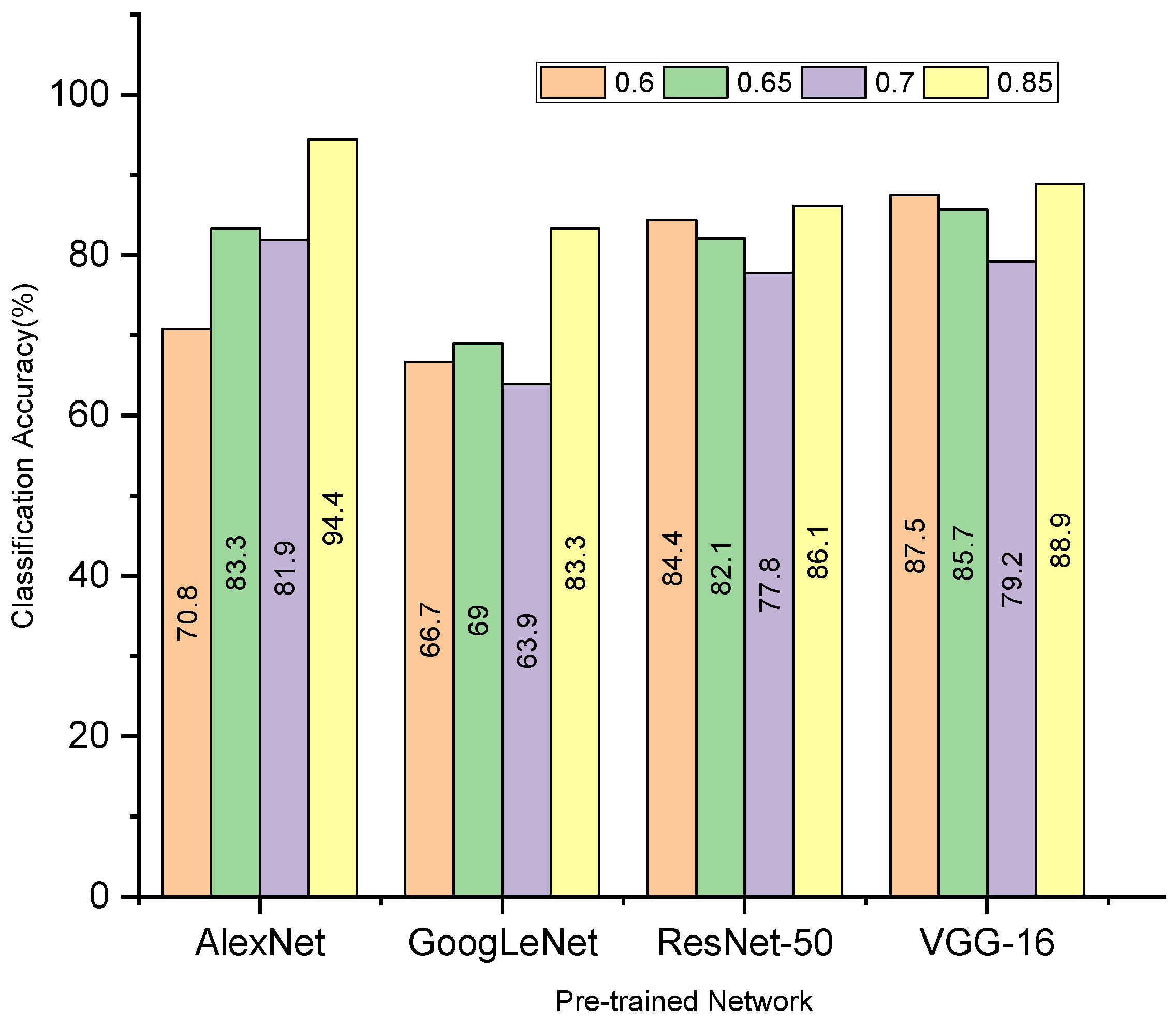
The resulting dataset was divided into two groups using the TR that was testing and training the data. The pretrained network was trained using training data, and the trained model was obtained for a specific dataset using testing data. Six TR were evaluated for the pretrained networks that this study looked at, and default settings for a number of hyperparameters were supplied to guarantee uniformity. For the purpose of determining the ideal TR, the hyperparameters 10 BS, 0.0001 LR, and SGDM SR were left unaltered. Figure 8 displays the results of many pretrained networks with various train–test split ratios.

Figure 8 demonstrates how the TR affects the performance of the pretrained network. Figure 8 shows that, for a TR of 0.85, AlexNet and GoogLeNet have the highest classification accuracies at 94.4% and 83.3%, respectively, while ResNet-50 and VGG-16 have the highest classification accuracies at 89.4% and 91.7 for a TR of 0.8, respectively.

6.2. Impact of Solvers

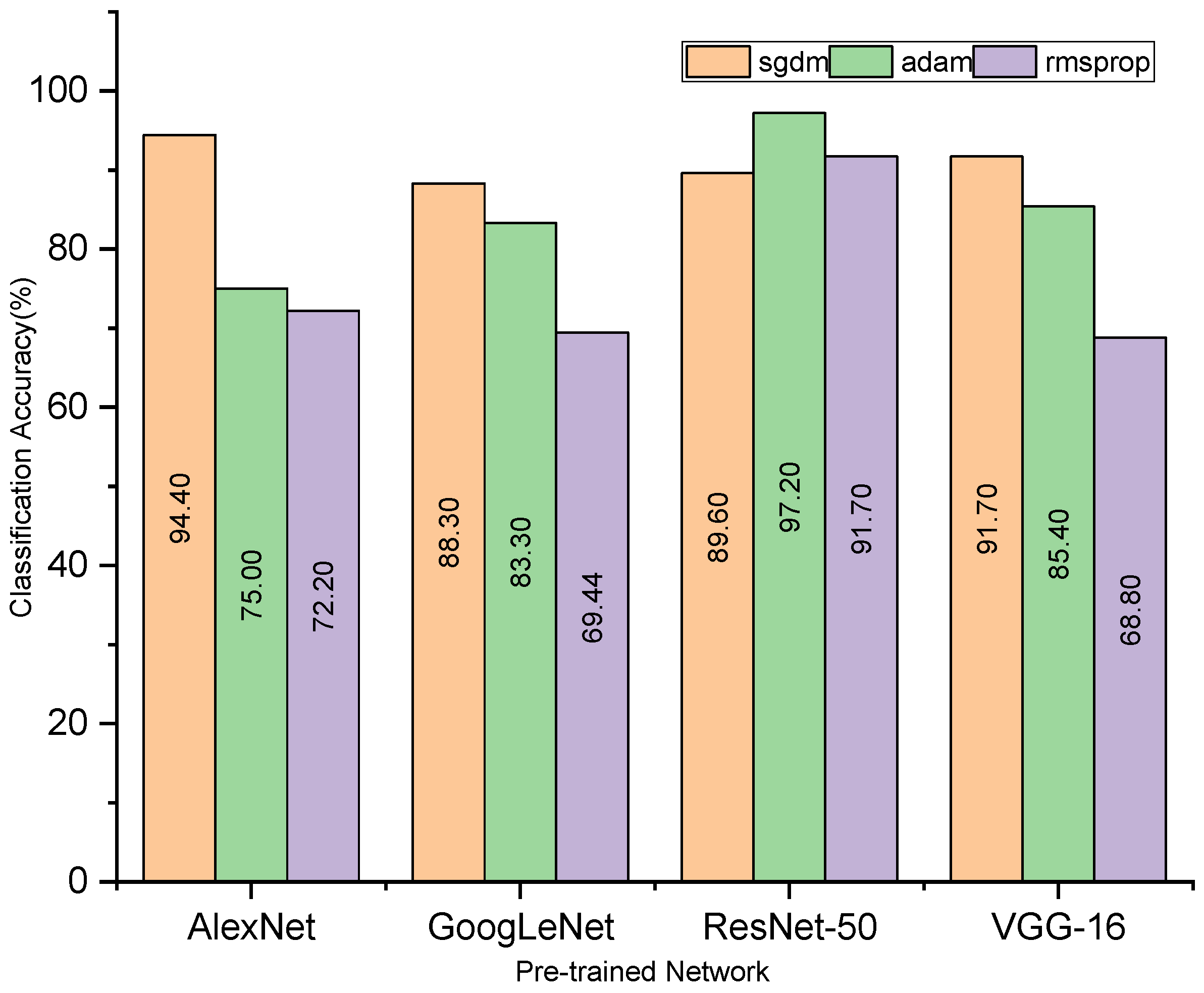
Algorithms used to minimize the loss value and improve the performance of the model during a training process are known as solvers or optimizers. Three different solvers (Adam, Sgdm and RMSprop) were used to examine the performance of the model. The best or ideal TR for each model was chosen to be 0.85 for AlexNet and GoogLeNet and 0.8 for VGG-16 and ResNet-50. Figure 9 shows the effectiveness of the pretrained model under various load conditions and solvers. By altering the optimizers, we can see how well the pretrained networks perform. From Figure 9 we are able to see that ResNet-50 has a classification accuracy of 97.2 and performed better when the Adam optimizer was used. GoogLeNet, AlexNet and VGG-16 acquired classification accuracies of 83.3%, 94.4% and 91.7%, respectively, and performed better when the sgdm solver was used.

6.3. Impact of Learning Rate (LR)

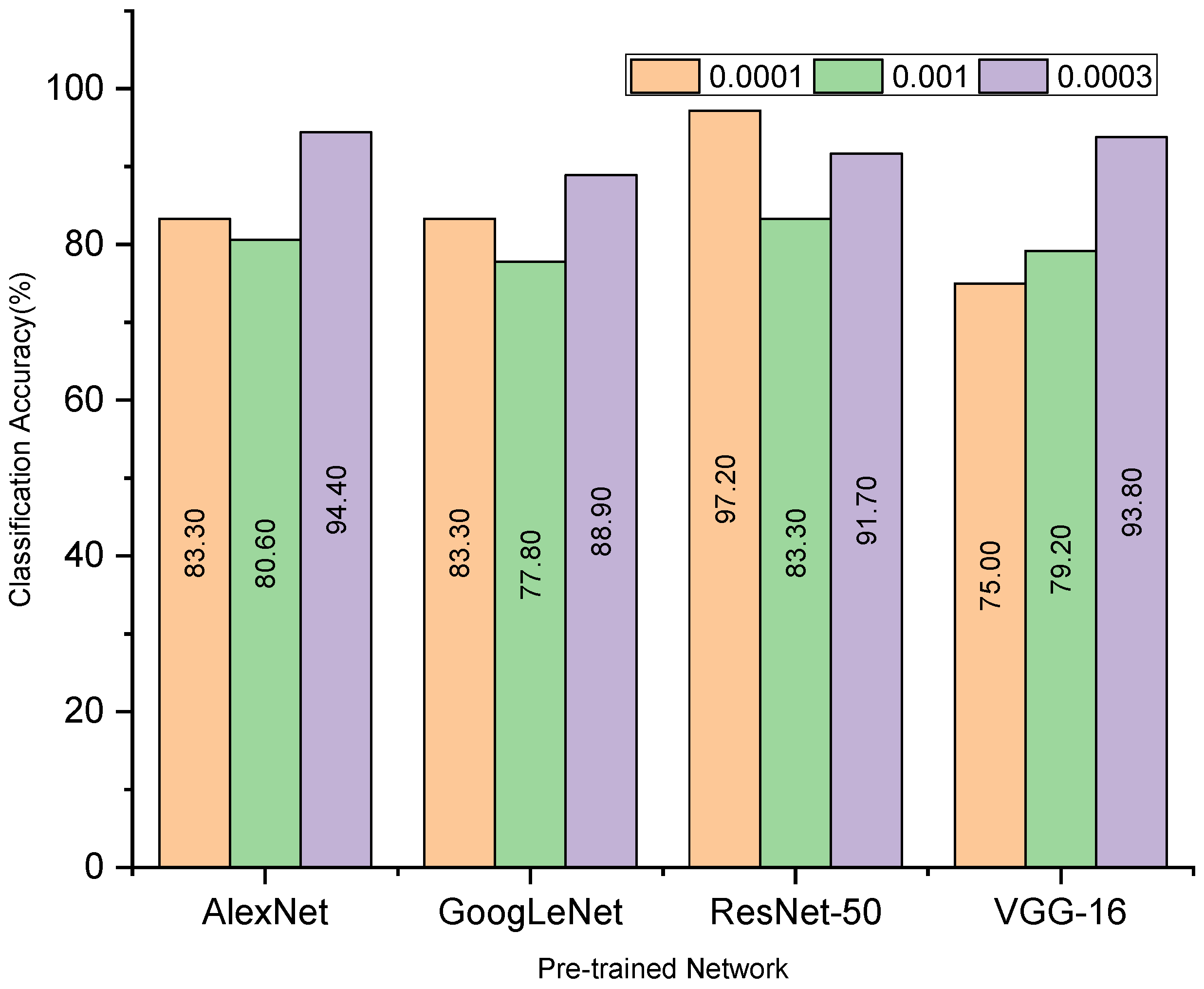
The learning rate is a hyperparameter that controls how much you update your network weights. The optimum learning rate may be difficult to identify since a low learning rate increases computation time while a high learning rate leads to wasteful training. This study employed three training rates (0.001, 0.0003, and 0.0001) to assess the performance of the model. For GoogLeNet and AlexNet, the hyperparameters were kept as (0.85 TR, sgdm solver), for ResNet-50 the hyperparameters were kept as (0.8 TR, Adam solver) and for VGG-16 the hyper parameters were kept as (0.8 TR and sgdm). The performances of the pretrained models at various degrees of learning rate are shown in Figure 10.

Figure 10 indicates that the performance of each pretrained network changes as the learning rate changes. AlexNet, GoogLeNet and VGG-16 each obtained a highest accuracy of 94.4%, 88.9% and 93.8%, respectively, at a learning rate of 0.0003. ResNet-50, on the other hand, achieved 97.2% classification accuracy and an LR of 0.0001. A model that categorizes items more accurately implies that it has learned the attributes efficiently and that the error value is lower.

6.4. Impact Batch Size (BS)

Batch size is a machine learning phrase that refers to the number of training samples used in one iteration. Batch normalization addresses a fundamental issue known as internal covariate shift. It assists in the appearance of data travelling across intermediate layers of the neural network, allowing you to apply a speedier learning pace. It has a regularizing effect, which means it may commonly eliminate dropout. Based on the experimental data reported in the preceding sections, the performance of the pretrained models used in this study was assessed using the top-performing hyperparameters for various BS (8, 10, 16, 24 and 32). The hyperparameters for GoogLeNet and AlexNet were retained at (0.85 TR, sgdm solver, 0.0003 LR), ResNet-50 at (0.8 TR, Adam solver, 0.0001), and VGG-16 at (0.8 TR, sgdm solver and 0.0003 LR). The performance of the pretrained models at various degrees of learning rate were shown in Figure 11.

Figure 11 demonstrates that altering the batch size has only minor impacts. For various batch sizes, every pretrained model showed an improvement in classification accuracy. For instance, ResNet-50 and AlexNet achieved 97.2% and 94.4% accuracy for batch sizes 10 and 16, respectively, whereas the Google Neural Network reached 83.3% accuracy for batch size 16. For a batch size of 32, VGG-16 obtained a total accuracy of 93.8% across all networks. The training process was sped up since a larger batch size implies less time spent training. The capacity of the network to generalize, however, declines as batch sizes increase.

6.5. Comparative Analysis of Trained Models

How to evaluate the effectiveness of pretrained neural networks is covered in this section.

Table 2. Best hyperparameters for the pretrained models.

Pretrained Model	Hyperparameters
	TR	BS	SR	LR
GoogLeNet	0.85	16	SGDM	0.0003
VGG-16	0.80	32	SGDM	0.0003
ResNet-50	0.80	10	ADAM	0.0001
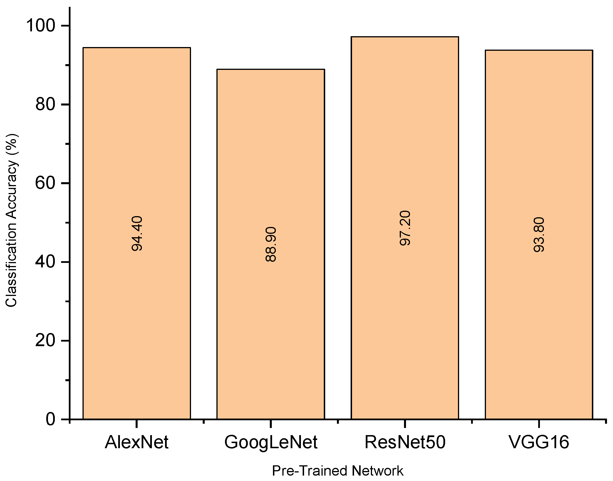
AlexNet	0.85	10	SGDM	0.0003

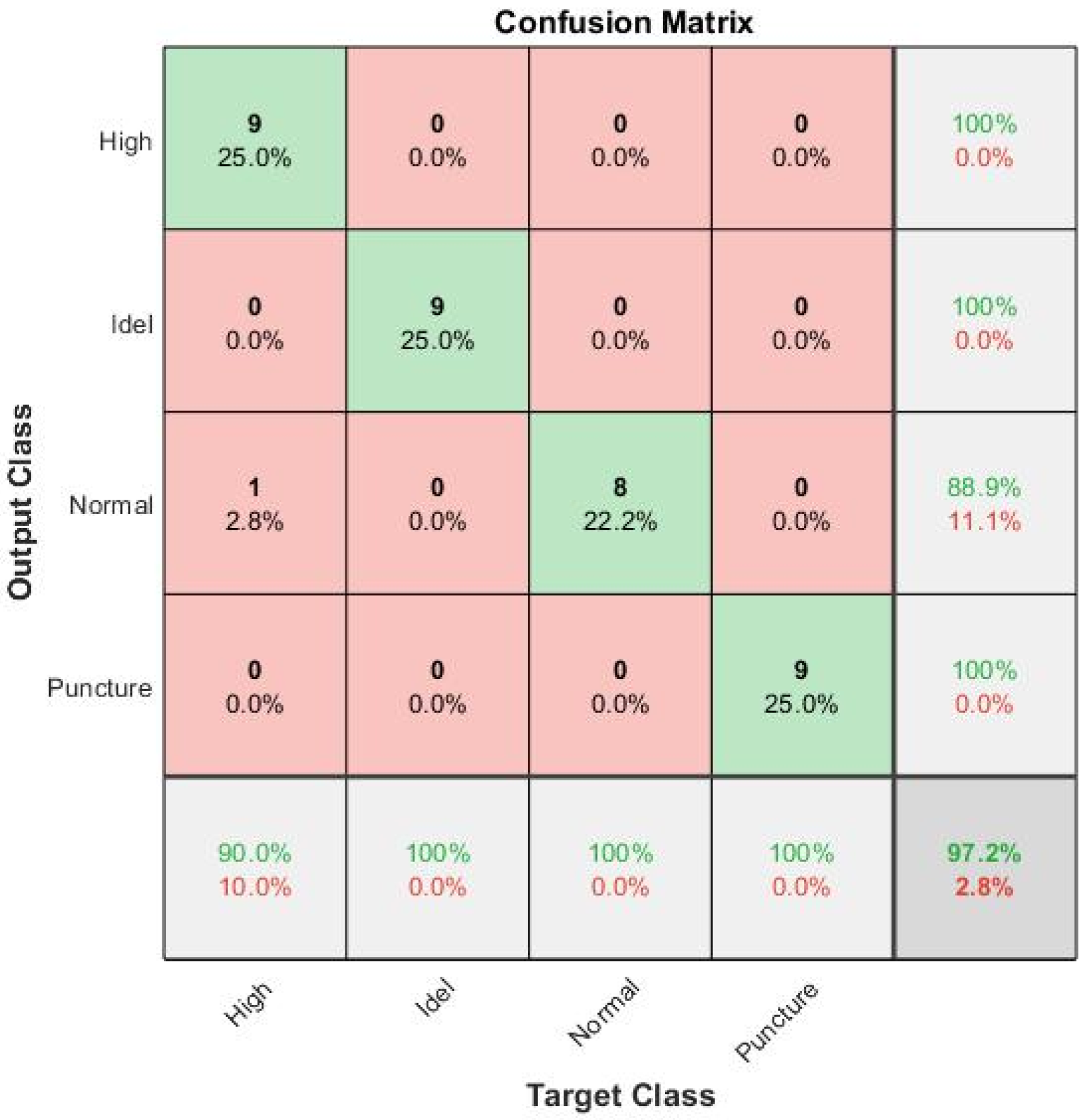
lists the ideal hyperparameters for enhancing the performance of the pretrained models based on the experimental findings from the preceding sections. The overall effectiveness of the pretrained networks with optimum hyperparameters is shown in Figure 12. Figure 12 illustrates the greatest performance of ResNet-50 for the specified ideal hyperparameters. Because of its overall better categorization, classification accuracy, and quicker processing times, ResNet-50 is advised for TPMS. The confusion matrix of the ResNet-50 design for TPMS is shown in Figure 13. The general performance level of a specific model or algorithm is shown via a confusion matrix. In relation to the examples categorized in the main diagonal, the confusion matrix was evaluated. The elements on the major diagonal reflect examples that were successfully categorized, whereas the other non-diagonal elements show occurrences that were incorrectly classified. According to the confusion matrices, the ResNet-50 architecture delivered correct classification accuracy for all situations with no misclassifications except normal (one instance is misclassified as high). Misclassification can occur for a variety of reasons, including noise interruption, poor signal quality, and signal similarity between recorded signals. The absence of misclassification instances implies that the network has learned all of the features well and that the loss during training is low. As a result of the observations obtained, ResNet-50 is recommended as the best-performing network for TPMS. 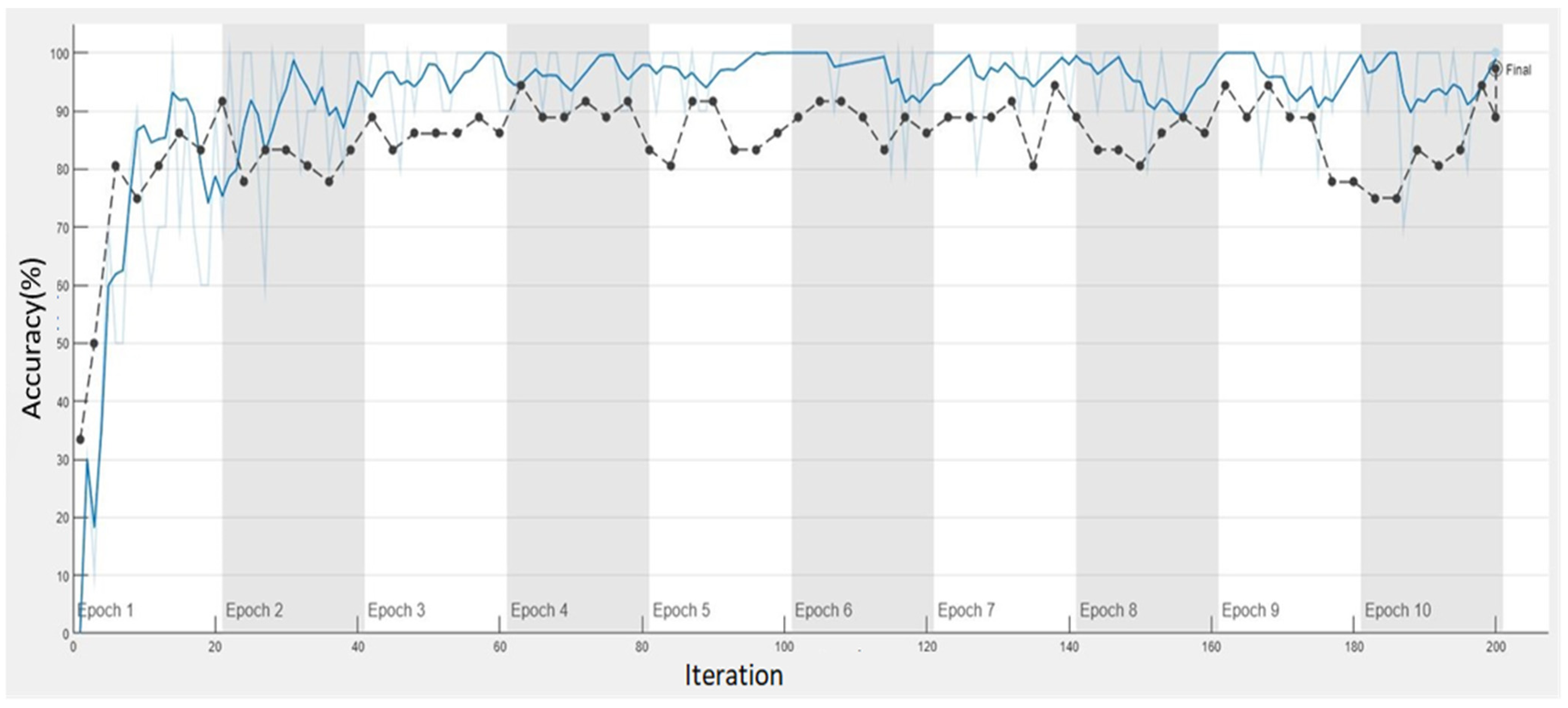Figure 14 represents the training process of ResNet-50 for TPMS. The pretrained networks with their best hyperparameters were evaluated with the help of a confusion matrix using AUC, precision, F1_score, specificity and accuracy, shown in

Table 3. Evaluation metrics for the pretrained networks.

Pretrained Network	Evaluation Metrics
	AUC	Precision	F1_Score	Specificity	Accuracy (%)
AlexNet	0.93	0.94	0.93	0.98	93.7
ResNet-50	0.84	0.97	0.97	0.99	97.2
GoogLeNet	0.71	0.82	0.82	0.94	82.9
VGG-16	0.93	0.93	0.93	0.98	93.4

.

6.6. Analyses of Other Innovative Works in Contrast

A comparison analysis was undertaken in this part to illustrate how the proposed approach outperforms other cutting-edge research accessible in the literature.

Table 4. Performance comparison using cutting-edge approaches.

	Classification Accuracy (%)	Reference
Random forest	95.00	[37]
Regression algorithm	91.25	[38]
random committee classifier	90.40	[39]
K-Star	89.16	[19]
Proposed methodology	97.20

compares the results of several methods to the recommended technique. Table 4 demonstrates that the proposed approach exceeds all previous works in the table by achieving a classification accuracy of 97.20%. The random forest method had the highest classification accuracy of 95.00%, followed by the regression algorithm, random committee classifier and K-star, which had values of 91.25%, 90.41% and 89.16% respectively.

7. Conclusions

This study talks about the integration of TPMS with a deep learning technique for better performance and accuracy. The condition of the tyre was determined using vibration plots with the help of a pretrained network. Four deep learning models—GoogLeNet, VGG-16, ResNet-50 and AlexNet—were employed in this study. High, Idle, Punctured and Normal test cases were considered in this study. The vibration signals were converted and processed by the pretrained network, which can deliver precise classification results. In order to provide a complete machine learning strategy, CNN layers comprise the pretrained networks that work together to accomplish classification, selection, and feature extraction. According to experimental findings, the adopted networks may learn complicated characteristics and provide credible classification results for analysing the TPMS. By tweaking a number of them, including the SR, TR, BS and LR, the optimum hyperparameters for each network were discovered. From the above results, we were able to conclude that ResNet-50 was the best performing network with 97.20% classification accuracy over the other suggested pretrained networks. One advantage of using deep learning techniques for TPMS is that they can effectively learn and extract features from the complex vibration signals, which may not be possible using traditional signal processing techniques. Additionally, the use of pretrained networks can reduce the amount of data and time required for training the models, making it a more efficient approach. However, one potential limitation of this approach is that it may require a large amount of labelled data to effectively train the models. Additionally, the accuracy of the models may be affected by factors such as variations in tyre and road conditions, which can affect the vibration signals. In terms of novelty, the study contributes to the growing body of research on using deep learning for TPMS. The use of multiple pretrained networks and hyperparameter tuning to achieve higher accuracy is a novel approach, and the study findings on the best-performing model (ResNet-50) can inform future research in this area.

Future works: There are several potential areas for future research that could build upon the findings of this study and further advance the use of deep learning in TPMS and related fields. One possibility is the development of more robust models that can handle variations in tyre and road conditions. Additionally, exploring the use of additional sensor data, such as temperature or pressure, could further improve the accuracy of the models. Another direction for future work could be investigating the feasibility of implementing this approach in real-time systems, such as in-vehicle TPMS. This could involve addressing challenges such as the need for real-time data processing and the limited computational resources available in these systems. Furthermore, utilizing LSTM instead of CNN could also be explored. The potential applications of this approach beyond TPMS could include predictive maintenance for other types of machinery that generate vibration signals.

References

- Mazur, V. Experimental Research in Automobile Non-Pneumatic Tire Force Heterogeneity. MATEC Web Conf. 2018, 224, 02019. [Google Scholar] [CrossRef]
- Popov, A.A.; Geng, Z. Modelling of Vibration Damping in Pneumatic Tyres. Veh. Syst. Dyn. 2005, 43, 145–155. [Google Scholar] [CrossRef]
- Abdulla, F.A.; Jebur, N.A.; Jasim, H.A. Effect of Using the Nitrogen in Automotive Tires on Vibration and Fuel Consumption. IOP Conf. Ser. Mater. Sci. Eng. 2020, 870, 012167. [Google Scholar] [CrossRef]
- Venkataraman, P. Effect of Nitrogen Filling on Tire Rolling Resistance and Vehicle Fuel Economy. Ph.D. Thesis, Clemson University, Clemson, SC, USA, 2007; p. 112. [Google Scholar]
- Waddell, W.H.; Napier, R.C.; Tracey, D.S. Nitrogen Inflation of Tires. Rubber Chem. Technol. 2009, 82, 229–243. [Google Scholar] [CrossRef]
- Praveen, H.; Sugumaran, V. Tyre Pressure Monitoring System—Machine Learning Approach. Recent Pat. Signal Process. 2015, 4, 84–93. [Google Scholar] [CrossRef]
- Kost, A.; Altabey, W.A.; Noori, M.; Awad, T. Applying Neural Networks for Tire Pressure Monitoring Systems. SDHM Struct. Durab. Health Monit. 2019, 13, 247–266. [Google Scholar] [CrossRef]
- Sachan, R.; Iqbal, S. Application of Machine Learning Technique for Development of Indirect Tire Pressure Monitoring System. SAE Int. J. Adv. Curr. Prac. Mobil. 2022, 4, 753–761. [Google Scholar] [CrossRef]
- Jiang, Z.; Liu, H.; Dai, Q. A New Intelligent Tire Pressure Monitoring System. In Proceedings of the 2011 International Conference of Information Technology, Computer Engineering and Management Sciences, Nanjing, China, 24–25 September 2011; Volume 2. [Google Scholar]
- Wang, X.; Chen, Z.; Cao, W.; Xu, G.; Liu, L.; Liu, S.; Li, H.; Shi, X.; Song, Q.; Xiao, Z.; et al. Artificial Neural Network-Based Method for Identifying Under-Inflated Tire in Indirect TPMS. IEEE Access 2020, 8, 213799–213805. [Google Scholar] [CrossRef]
- Wagh, M.V.; Pawal, A.; Sharama, S.; Patil, H. A Survey on Tire Pressure Monitoring System. IJAREEIE 2018, 7, 4031–4035. [Google Scholar]
- Jerry, H. Robinson, III. Remote tire pressure monitoring system employing coded tire identification and radio frequency transmission and enabling recalibration upon tire rotation or replacement. US Patent US5838229A, 17 November 1998. Available online: https://patents.google.com/patent/US5838229/ (accessed on 1 January 2023).
- Craighead, I.A. Sensing Tyre Pressure, Damper Condition and Wheel Balance from Vibration Measurements. Proc. Inst. Mech. Eng. Part D J. Automob. Eng. 1997, 211, 265–297. [Google Scholar] [CrossRef]
- Chandolikar, N.S.; Nandavadekar, V.D. Investigation of Feature Selection and Ensemble Methods For Performance Improvement of Intrusion Attack Classification. Int. J. Appl. Chem. Pharm. Sci. 2013, 2, 131–136. [Google Scholar]
- Aravinthasamy, V.; Vijay Kumar Yadav, R.; Tharani Tharan, B.; Viknesh, R.; Mahendran, K. Tyre Pressure Monitoring System Using Wireless Communication. Int. J. Pure Appl. Math. 2018, 118, 895–900. [Google Scholar]
- Marton, Z.; Fodor, D.; Enisz, K.; Nagy, K. Frequency Analysis Based Tire Pressure Monitoring. In Proceedings of the 2014 IEEE International Electric Vehicle Conference (IEVC), Florence, Italy, 17–19 December 2014. [Google Scholar]
- Wu, B.; Fang, Y.; Deng, L. Summary of Energy Collection Application in Vehicle Tire Pressure Monitoring System. In Proceedings of the CACRE2019: Proceedings of the 2019 4th International Conference on Automation, Control and Robotics Engineering, Shenzhen, China, 19–21 July 2019. [Google Scholar]
- Anoop, P.S.; Sugumaran, V. Effect of Wheel Balancing on Tyre Condition Monitoring System Using Vibration Signals through Statistical Features and Machine Learning Techniques. J. Intell. Fuzzy Syst. 2022, 43, 561–573. [Google Scholar] [CrossRef]
- Anoop, P.S.; Sugumaran, V.; Mithun Praveen, H. Implementing K-Star Algorithm to Monitor Tyre Pressure Using Extracted Statistical Features from Vertical Wheel Hub Vibrations. Indian J. Sci. Technol. 2016, 9, 1–7. [Google Scholar] [CrossRef]
- Anoop, P.S.; Sugumaran, V. Classifying Machine Learning Features Extracted from Vibration Signal with Logistic Model Tree to Monitor Automobile Tyre Pressure. SDHM Struct. Durab. Health Monit. 2017, 11, 191–208. [Google Scholar] [CrossRef]
- He, K.; Zhang, X.; Ren, S.; Sun, J. Deep Residual Learning for Image Recognition. In Proceedings of the 2016 IEEE Conference on Computer Vision and Pattern Recognition (CVPR), Las Vegas, NV, USA, 27–30 June 2016; pp. 770–778. [Google Scholar] [CrossRef]
- Szegedy, C.; Liu, W.; Jia, Y.; Sermanet, P.; Reed, S.; Anguelov, D.; Erhan, D.; Vanhoucke, V.; Rabinovich, A. Going Deeper with Convolutions. In Proceedings of the Proceedings of the IEEE Computer Society Conference on Computer Vision and Pattern Recognition, Boston, MA, USA, 7–12 June 2015. [Google Scholar]
- Simonyan, K.; Zisserman, A. Very Deep Convolutional Networks for Large-Scale Image Recognition. In Proceedings of the 3rd International Conference on Learning Representations, ICLR 2015, San Diego, CA, USA, 7–9 May 2015; pp. 1–14. [Google Scholar]
- Asha, P.; Natrayan, L.; Geetha, B.T.; Beulah, J.R.; Sumathy, R.; Varalakshmi, G.; Neelakandan, S. IoT Enabled Environmental Toxicology for Air Pollution Monitoring Using AI Techniques. Environ. Res. 2022, 205, 112574. [Google Scholar] [CrossRef]
- Ding, X.; He, Q. Energy-Fluctuated Multiscale Feature Learning with Deep ConvNet for Intelligent Spindle Bearing Fault Diagnosis. IEEE Trans. Instrum. Meas. 2017, 66, 1926–1935. [Google Scholar] [CrossRef]
- Lee, D.; Siu, V.; Cruz, R.; Yetman, C. Convolutional Neural Net and Bearing Fault Analysis; CSREA Press: Providence, RI, USA, 2016; pp. 194–200. [Google Scholar]
- Hoang, D.T.; Kang, H.J. Rolling Element Bearing Fault Diagnosis Using Convolutional Neural Network and Vibration Image. Cogn. Syst. Res. 2019, 53, 42–50. [Google Scholar] [CrossRef]
- Wen, L.; Li, X.; Gao, L.; Zhang, Y. A New Convolutional Neural Network-Based Data-Driven Fault Diagnosis Method. IEEE Trans. Ind. Electron. 2018, 65, 5990–5998. [Google Scholar] [CrossRef]
- Verma, N.K.; Gupta, V.K.; Sharma, M.; Sevakula, R.K. Intelligent Condition Based Monitoring of Rotating Machines Using Sparse Auto-Encoders. In Proceedings of the 2013 IEEE Conference on Prognostics and Health Management (PHM), Gaithersburg, MD, USA, 24–27 June 2013. [Google Scholar]
- Wang, Z.; Wang, J.; Wang, Y. An Intelligent Diagnosis Scheme Based on Generative Adversarial Learning Deep Neural Networks and Its Application to Planetary Gearbox Fault Pattern Recognition. Neurocomputing 2018, 310, 213–222. [Google Scholar] [CrossRef]
- Liu, G.; Bao, H.; Han, B. A Stacked Autoencoder-Based Deep Neural Network for Achieving Gearbox Fault Diagnosis. Math. Probl. Eng. 2018, 2018, 5105709. [Google Scholar] [CrossRef]
- Liu, H.; Zhou, J.; Zheng, Y.; Jiang, W.; Zhang, Y. Fault Diagnosis of Rolling Bearings with Recurrent Neural Network-Based Autoencoders. ISA Trans. 2018, 77, 167–178. [Google Scholar] [CrossRef] [PubMed]
- Lee, W.J.; Mendis, G.P.; Sutherland, J.W. Development of an Intelligent Tool Condition Monitoring System to Identify Manufacturing Tradeoffs and Optimal Machining Conditions. Procedia Manuf. 2019, 33, 256–263. [Google Scholar] [CrossRef]
- Elangovan, M.; Devasenapati, S.B.; Sakthivel, N.R.; Ramachandran, K.I. Evaluation of Expert System for Condition Monitoring of a Single Point Cutting Tool Using Principle Component Analysis and Decision Tree Algorithm. Expert Syst. Appl. 2011, 38, 4450–4459. [Google Scholar] [CrossRef]
- Balazinski, M.; Czogala, E.; Jemielniak, K.; Leski, J. Tool Condition Monitoring Using Artificial Intelligence Methods. Eng. Appl. Artif. Intell. 2002, 15, 73–80. [Google Scholar] [CrossRef]
- Rangwala, S.; Dornfeld, D. Sensor Integration Using Neural Networks for Intelligent Tool Condition Monitoring. J. Manuf. Sci. Eng. Trans. ASME 1990, 112, 219–228. [Google Scholar] [CrossRef]
- Anoop, P.S.; Sugumaran, V. The Influence of Tyre Balancing in Nitrogen Filled Tyres Using Statistical Features and Random Forest Algorithm. Int. J. Mech. Prod. Eng. Res. Dev. 2020, 10, 6679–6690. [Google Scholar] [CrossRef]
- Han, B.; Ji, S.; Wang, J.; Bao, H.; Jiang, X. An Intelligent Diagnosis Framework for Roller Bearing Fault under Speed Fluctuation Condition. Neurocomputing 2021, 420, 171–180. [Google Scholar] [CrossRef]
- Anoop, P.S.; Nair, P.; Sugumaran, V. Influence of Unbalance on Classification Accuracy of Tyre Pressure Monitoring System Using Vibration Signals. SDHM Struct. Durab. Health Monit. 2021, 15, 261–279. [Google Scholar] [CrossRef]