A Novel Rotor Position Observer for Sensorless Control of Permanent Magnet Synchronous Motor Based on Adaptive Generalized Second-Order Integrator

Abstract

In order to realize sensorless control of permanent magnet synchronous motor (PMSM) with high performance in low speed region, a novel rotor position observer scheme based on finite control set model predictive control (FCS-MPC) is presented in this paper. Firstly, the FCS-MPC is used to predict the current and drive the PMSM by selecting the optimal control quantity that minimizes the cost function. Next, an adaptive second-order generalized integrator (ASOGI) with adaptive center frequency adjustment was designed to replace the band-pass filter (BPF) in the rotor position observer. The ASOGI can calculate the high frequency value that can be used for position estimation by the controller switching frequency. The current ripple inherent in the FCS-MPC is considered as the response current obtained by the high frequency injection (HFI) method. The current ripple after ASOGI filtering is input to the phase-locked loop (PLL) for phase locking to obtain the estimated rotor position. In addition, adaptive linear (Adaline) neural networks are used to identify sensitive motor parameters online to avoid mismatch of model parameters, which causes degradation of control performance. Simulation experiments and hardware experiments show that this scheme is excellent in both static and dynamic conditions.

1. Introduction

Permanent magnet synchronous motor (PMSM) has the advantages of high power density, quick dynamic response, and great efficiency [1,2]. With the advancement in microprocessors, predictive control is widely applied to the high-performance control of PMSM [3]. Finite control set model predictive control (FCS-MPC) uses the discrete quality of the inverter switching states to control the motor by selecting the switching state that minimizes the value of the cost function from a finite number of alternative switching states [4,5], eliminating the need for pulse width modulation (PWM) modulation and generating the drive signal directly. Although the model predictive control has many advantages, in practical applications, the computational delay of the digital implementation brings degradation to the system performance. In [6], the one-step delay compensation method in [7] was used to calculate the current compensation term using Heun’s method for the action delay problem, which improved the prediction accuracy of current values. The reference voltage is obtained by Deadbeat principle and the number of calculations for the non-zero vector is reduced from 18 to 4 when selecting the optimal voltage vector and its duty cycle, which greatly reduces the computational burden. In [8], the prediction model is updated with the current in the α-β subspace at moment k + 1 as the compensation current to obtain the prediction model at moment k + 2. Therefore, it is necessary to take measures to compensate the MPC controller. Similar to field-oriented control, rotor position is also very important in model predictive control [9]. However, traditional mechanical position sensors have problems such as high installation cost and low reliability [10]. Therefore, sensorless control has gradually become a new control method for PMSM [11]. Due to the small back electromotive force (EMF) of PMSM in the low speed region, the rotor position is usually estimated using the high-frequency injection (HFI) method [12,13]. Ref. [14] adopts a hybrid control strategy to achieve smooth switching from low speed to high speed. The high-frequency signal injection method is used to effectively extract the back EMF signal at a low speed, and then the finite-position-set-phase-locked loop (FPS-PLL) with high accuracy and robustness is used at high speed. However, the HFI will inevitably generate torque ripple and increased loss, and the dynamic performance will be insufficient when the load torque and speed suddenly change [15,16]. The choice of discrete switching states by the FCS-MPC creates an inherent high-frequency current ripple [17], and this inherent characteristic can replace the additional signal in the sensorless control which can be regarded as the response current generated on the q-axis when the d-axis is excited, so that the motor produces a saturated saliency [18,19,20]. In [21], the traditional vector control is replaced by the more advanced model predictive control. The combination of MPC and FPS-PLL makes the controller structure simple and has better dynamic stability performance. The FPS-PLL can directly search for the rotor position angle without adjusting the parameters of the PI controller. Using filters to process the inherent current ripple is an essential step in the rotor position estimation. In [22], a PLL with a modified control function is combined with FCS-MPC, which avoids the wrong estimation during speed reversal conditions as well as singularities. Unlike the fixed frequency injection signal of HFI, the switching frequency of FCS-MPC is not constant. There are a large number of changing high-frequency harmonics and noise, which makes it difficult to extract the signal at a specific frequency accurately in the current ripple with changing frequency by directly using the band-pass filter (BPF). The phase offset of the BPF will cause deviations in the estimation result of the rotor position [23]. The second-order generalized integrator (SOGI) has a simple structure without time delay which, combined with PLL, can eliminate direct current (DC) offset and harmonics well to realize accurate estimation of rotor position [24]. The SOGI can improve the dynamic performance of sensorless control at low speeds [25,26].

In addition, MPC performs predictive control based on an accurate mathematical model, and changes in the external environment and motor operating conditions may cause changes in motor parameters, resulting in model mismatch [27,28,29]. It is necessary to identify and modify the sensitive parameters such as the inductance and flux linkage of the motor online to correct the preset parameters of the model [30].

An adaptive second-order generalized integrator (ASOGI)-PLL structure is proposed to realize sensorless control of PMSM in this paper. The main contributions are shown as below:

• The rotor position is estimated using the inherent current ripple of the FCS-MPC instead of the externally injected high-frequency signal.
• The center frequency of the ASOGI can be adaptively varied to adaptively filter the inherent current ripple with large frequency fluctuations, and it is used instead of the BPF.
• The parameters of the controller are corrected online using Adaptive linear (Adaline) neural network.

The experimental results show that the proposed method can accurately estimate the rotor position at low and even ultra-low speeds of PMSM. The PMSM has good load carrying and anti-disturbance capability.

This paper is organized as follows: Section 2 analyzes the mathematical model and the inherent current ripple of the PMSM at finite control set model predictive control. Section 3 presents the ASOGI-PLL structure for rotor position estimation and uses Adaline to correct the controller parameters. The simulation and experimental results are presented in Section 4. Finally, Section 5 gives the conclusion of this paper.

2. MPC Mathematical Model of Permanent Magnet Synchronous Motor

In this section, the mathematical model of the PMSM under finite control set model predictive control is first established. In order to extract the rotor position using the intrinsic current ripple, the inherent current ripple is further analyzed.

2.1. FCS-MPC Mathematical Model

The coordinate system of permanent magnet synchronous motor is shown in Figure 1. ABC is the three-phase coordinate system, α-β is the stationary coordinate system, d-q is the rotational coordinate system, $\theta$ is the angle between the rotor, and the A(α) axis, the $\widehat{d}$ axis is defined as the estimated d-axis and the $\widehat{q}$ axis is the estimated q-axis, $\widehat{\theta }$ is the angle between the $\widehat{d}$ axis and the A(α) axis, the estimated angular error is $\mathsf{\Delta }\theta =\theta -\widehat{\theta }$, N and S are the polarities.

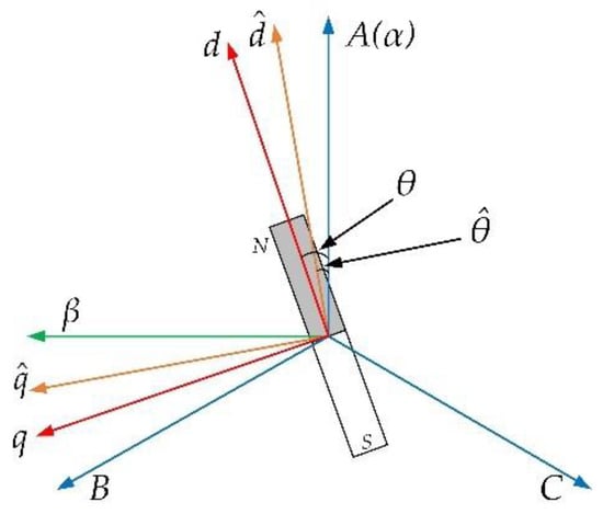
Figure 1. Coordinate system of PMSM.

The voltage equation of PMSM in the d-q rotating coordinate system can be expressed as

$$\{\begin{array}{l}{u}_d=L_d\frac{d{i}_d}{dt}-\omega L_q{i}_q+R{i}_d\\ u_q=\omega L_d{i}_d+L_q\frac{d{i}_q}{dt}+\omega {\phi }_{\mathrm{f}}+R{i}_q\end{array}$$

(1)

where u_d and u_q are the d and q axes voltages, i_d and i_q are the d and q axes currents in the synchro-nous rotation coordinate system, respectively, ${\phi }_{\mathrm{f}}$ is the rotor permanent magnet flux linkage, $\omega$ is the rotor angular velocity, L_d and L_q are the motor straight-axis inductance and cross-axis inductance, respectively, and R is the stator resistance.

The schematic diagram of the model predictive control of the PMSM is shown in Figure 2. The i_d^* and i_q^* are reference currents on the d and q axes, respectively.

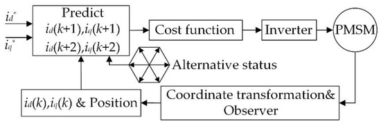
Figure 2. PMSM predictive control schematic.

In the finite set model predictive control, the controlled object is a discretized model, and the d and q axes currents are chosen as state variables, and the predicted currents are obtained by discretizing (1) using Euler method at the k moment.

$$\{\begin{array}{l}{i}_d(k+1)=i_d^M(k)+\frac{T_s}{L_d}[u_d(k)-R{i}_d^M(k)+\omega (k)L_q{i}_q^M(k)]\\ i_q(k+1)=i_q^M(k)+\frac{T_s}{L_q}[u_q(k)-R{i}_q^M(k)+\omega (k)L_d{i}_d^M(k)-\omega (k){\phi }_{\mathrm{f}}]\end{array}$$

(2)

where the superscript M denotes the measured value, T_s is the sampling period. The output of the inverter circuit S_abc represents the eight switching states of the inverter under discrete control, consisting of six non-zero voltage vectors and two zero voltage vectors, expressed as

$$V\in \{V_0,V_1,V_2,V_3,V_4,V_5,V_6,V_7\}$$

(3)

where V denotes the alternative switching state, V₁ to V₆ are non-zero voltage vectors, and V₀ and V₇ denote zero voltage vectors.

Due to the computational delay in the digital implementation, a two-step approach is generally used to compensate for the one-step controller delay. After using Equation (2) to obtain the predicted current at moment k + 1, we then used Equation (3) to predict the current at moment k + 2 for each of the eight S_abc states.

$$\{\begin{array}{l}{i}_d(k+2)=i_d^M(k+1)+\frac{T_s}{L_d}[u_d(k+1)-R{i}_d^M(k+1)+\omega (k+1)L_q{i}_q^M(k+1)]\\ i_q(k+2)=i_q^M(k+1)+\frac{T_s}{L_q}[u_q(k+1)-R{i}_q^M(k+1)+\omega (k+1)L_d{i}_d^M(k+1)-\omega (k+1){\phi }_{\mathrm{f}}]\end{array}$$

(4)

The controller traverses the discrete switching states. Since the sampling interval is extremely short, the current loop is given a reference current $i_d^{\ast }$, $i_q^{\ast }$ constant for adjacent moments. Construct the cost function based on the value at moment k and the predicted value at moment k + 2

$$J=[i_d^{\ast }-i_d^{}(k+2{\left)\right]}^2+\lambda {[i_q^{\ast }-i_q^{}(k+2)]}^2$$

(5)

where $\lambda$ is the weighting factor, which is generally taken as 1.

The voltage vector that minimizes the cost function is selected as the optimal voltage vector, and the corresponding u_d(k + 1), u_q(k + 1) and the optimal switch combination are obtained for rolling the next control cycle roll. Since the set of alternative switching states is fixed and discrete, it is finite control set as discrete control.

2.2. Inherent Current Ripple of FCS-MPC

The discrete switching control traverses each switching state at each control cycle in Figure 3, corresponding to seven different spatial voltage vectors. The processor needs to calculate the cost function which corresponds to the predicted current generated by each voltage vector, which inevitably creates the high-frequency current ripple inherent in FCS-MPC control.

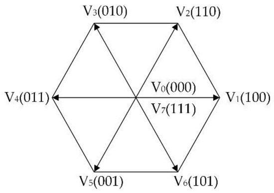
Figure 3. Spatial voltage vector.

In the motor synchronous rotation coordinate system, the current relationship between d-q axis and $\widehat{d}-\widehat{q}$ axis is

$$\{\begin{array}{l}{\widehat{i}}_d=i_d\cos \mathsf{\Delta }\theta -i_q\sin \mathsf{\Delta }\theta \\ {\widehat{i}}_q=i_d\sin \mathsf{\Delta }\theta +i_q\cos \mathsf{\Delta }\theta \end{array}$$

(6)

Similarly, the voltage relationship between d-q axis and $\widehat{d}-\widehat{q}$ axis is

$$\{\begin{array}{l}{\widehat{u}}_d=u_d\cos \mathsf{\Delta }\theta -u_q\sin \mathsf{\Delta }\theta \\ {\widehat{u}}_q=u_d\sin \mathsf{\Delta }\theta +u_q\cos \mathsf{\Delta }\theta \end{array}$$

(7)

The term $u_d(k)-R{i}_d(k)+\omega (k)L_q{i}_q(k)$ in (2) is written as U_D and the term $u_q(k)-R{i}_q(k)+\omega (k)L_d{i}_d(k)-\omega (k){\phi }_{\mathrm{f}}$ is written as U_Q, therefore the predicted current on the d-q axis at moment k + 1 is

$$\{\begin{array}{l}{i}_d(k+1)=i_d(k)+U_D{T}_s/L_d\\ i_q(k+1)=i_q(k)+U_Q{T}_s/L_q\end{array}$$

(8)

The PMSM produces saturated convex polarity under high frequency excitation, so that the inherent current ripple can be used as a high frequency characteristic instead of external high frequency voltage injection to produce high frequency response currents, and thus the position observer can be designed to extract the rotor position contained in the current ripple. In order to make the current ripple high frequency signal more significant and stable, the frequency distribution range of the current ripple is usually reduced using the adjacent vector voltage selection method. As shown in Table 1, the optimal switching state for the next moment that minimizes the cost function is selected from two adjacent valid zero vectors using the switching combination of the previous moment.

Table 1. Switch Status Table.

Previous States	Alternate States
000 (V0)	100	010	001
100 (V1)	000	110	101
110 (V2)	010	100	111
010 (V3)	110	000	011
011 (V4)	111	001	010
001 (V5)	000	011	101
101 (V6)	001	111	100
111 (V0)	011	101	110

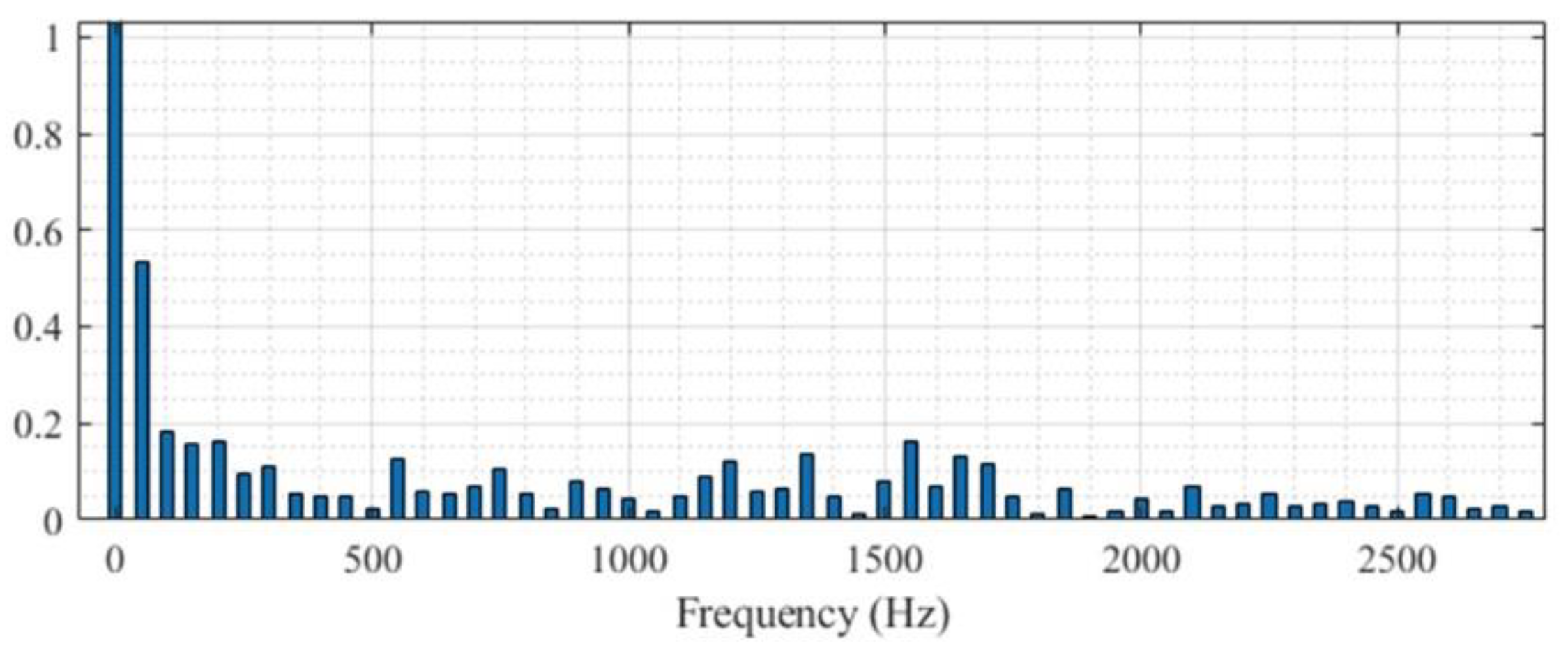
We started the PMSM from static to 150 r/min (10% of the rated speed) with 50% of the rated load. The d-q axis currents at moment k were obtained by Park’s transformation after collecting three-phase currents, and the FFT analysis of motor phase currents is shown in Figure 4. The current contains high-frequency current components that are much higher than the fundamental frequency. It can be seen that this method makes the frequency of the high-frequency part of the current ripple mostly concentrated in 500 Hz~2000 Hz. However, due to the discrete switching characteristics, the frequencies of the currents are not fixed, and the harmonic dispersion is more chaotic, which causes some difficulties in the selection and extraction of the filter cutoff frequency and affects the estimation of rotor position.

Figure 4. A-phase current FFT analysis.

3. ASOGI-PLL Rotor Position Observer

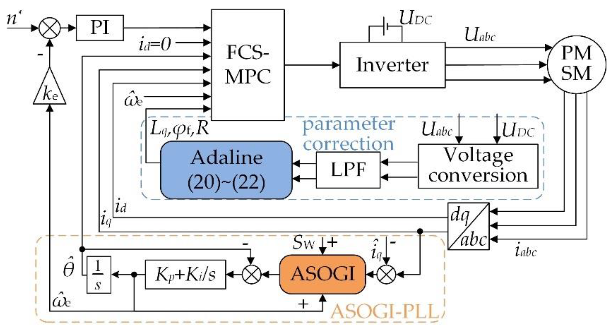
In this section, a novel rotor observation structure is proposed. To solve the problem that the BPF cannot adapt to the frequent changes of the inherent current ripple frequency, the ASOGI with adaptive center frequency selection is designed. The ASOGI-PLL can accurately estimate the rotor position. Furthermore, Adaline linear neural network is used to correct the MPC parameters to avoid the system performance degradation.

3.1. Conventional PLL Rotor Position Observer

In the $\widehat{d}-\widehat{q}$ axis, the predicted current expression from (2) is

$$\{\begin{array}{l}{\widehat{i}}_d(k+1)={\widehat{i}}_d^M(k)+\frac{T_{\mathrm{s}}}{L_d}[{\widehat{u}}_d(k)-R{\widehat{i}}_d^M(k)+\widehat{\omega }(k)L_q{\widehat{i}}_q^M(k)]\\ {\widehat{i}}_q(k+1)={\widehat{i}}_q^M(k)+\frac{T_{\mathrm{s}}}{L_q}[{\widehat{u}}_q(k)-R{\widehat{i}}_q^M(k)+\widehat{\omega }(k)L_d{\widehat{i}}_d^M(k)-\widehat{\omega }(k){\phi }_{\mathrm{f}}]\end{array}$$

(9)

From (6), the measured value of the current in the $\widehat{d}-\widehat{q}$ axis can be expressed as

$$\{\begin{array}{l}{\widehat{i}}_d^M(k+1)=i_d(k+1)\cos \mathsf{\Delta }\theta -i_q(k+1)\sin \mathsf{\Delta }\theta \\ {\widehat{i}}_q^M(k+1)=i_d(k+1)\sin \mathsf{\Delta }\theta +i_q(k+1)\cos \mathsf{\Delta }\theta \end{array}$$

(10)

In the present control cycle, the current error between the estimated value and the measured value is obtained from (9) and (10) as

$$\mathsf{\Delta }{i}_d(k+1)={\widehat{i}}_d^M(k+1)-{\widehat{i}}_d(k+1)$$

(11)

$$\mathsf{\Delta }{i}_q(k+1)={\widehat{i}}_q^M(k+1)-{\widehat{i}}_q(k+1)$$

(12)

Due to the extremely short sampling time, the k and k + 1 moments can be considered as steady states, and the current error on the q-axis is obtained by substituting (6) to (10) into (12) and simplifying

$$\mathsf{\Delta }{i}_q(k+1)=T_s(\frac{U_D}{L_d}-\frac{U_D}{L_q})\sin \mathsf{\Delta }\theta$$

(13)

The position error information is included in (13), and the motor parameters can be regarded as constants within a control cycle, U_D and U_Q can be used as control constants without the interference of nonlinearity, and the interference of the cosine term is excluded by establishing the q-axis current error correlation term.

Considering the rotor position information contained in the q-axis error current and the effect of the d-axis current, the rotor position angle error term is established and derived according to (8) and (13).

$$\epsilon (k)=[{\widehat{i}}_q^M(k)-{\widehat{i}}_q(k)]{\widehat{U}}_D=T_s[\frac{1}{L_d}-\frac{1}{L_q}]U_D^2\sin \mathsf{\Delta }\theta \cos \mathsf{\Delta }\theta -T_s[\frac{1}{L_d}-\frac{1}{L_q}]U_D{U}_Q{\sin }^2\mathsf{\Delta }\theta$$

(14)

Due to the orthogonality of d-axis and q-axis, U_D and U_Q are not correlated with each other. In the steady state, U_D and U_Q are not constant at zero value in the discrete switch control steady state, but their average values ${\overline{U}}_D=0$, ${\overline{U}}_Q=0$. Therefore, the second term in (14) is approximately equal to zero, giving a function on $\mathsf{\Delta }\theta$

$$\epsilon (\mathsf{\Delta }\theta )=\frac{T_s}{2}[\frac{1}{L_d}-\frac{1}{L_q}]U_D^2\sin (2\mathsf{\Delta }\theta )=K_e\sin (2\mathsf{\Delta }\theta )$$

(15)

where $K_e$ is a constant.

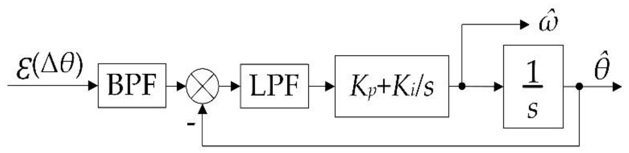
When the estimated rotor position is true, the $\widehat{d}$ axis coincides with the $\widehat{q}$ axis, $\mathsf{\Delta }\theta =0$, and (15) is also zero. Use the PLL in Figure 5 to lock the phase contained in (15).

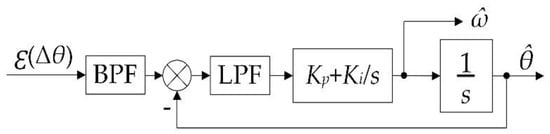
Figure 5. Phase locked loop structure diagram.

In the HFI method, the high frequency signal is usually processed by BPF first, and the center frequency of the BPF is kept the same as the frequency of the injected signal. However, in FCS-MPC, the frequency of the high-frequency signal is not stable and is accompanied by high-frequency harmonics. The conventional second-order BPF has the defects of phase shift and fixed center frequency, so it is necessary to design a filter that can adapt to the high-frequency signal with varying current ripple and minimize the phase shift, and then perform phase locking through the PLL structure to obtain the rotor position.

3.2. ASOGI-PLL Rotor Position Observer

The SOGI structure is shown in Figure 6. The transfer function can be expressed as

$$D(s)=\frac{v^{\prime }(s)}{v(s)}=\frac{l{\omega }_{\mathrm{c}}s}{s^2+l{\omega }_{\mathrm{c}}s+{\omega }_{\mathrm{c}}{}^2}$$

(16)

where l is the damping factor, ${\omega }_{\mathrm{c}}$ is the center frequency, $v$ is the input signal, $v^{\prime }$ and $q{v}^{\prime }$ are output signal.

Figure 6. SOGI structure diagram.

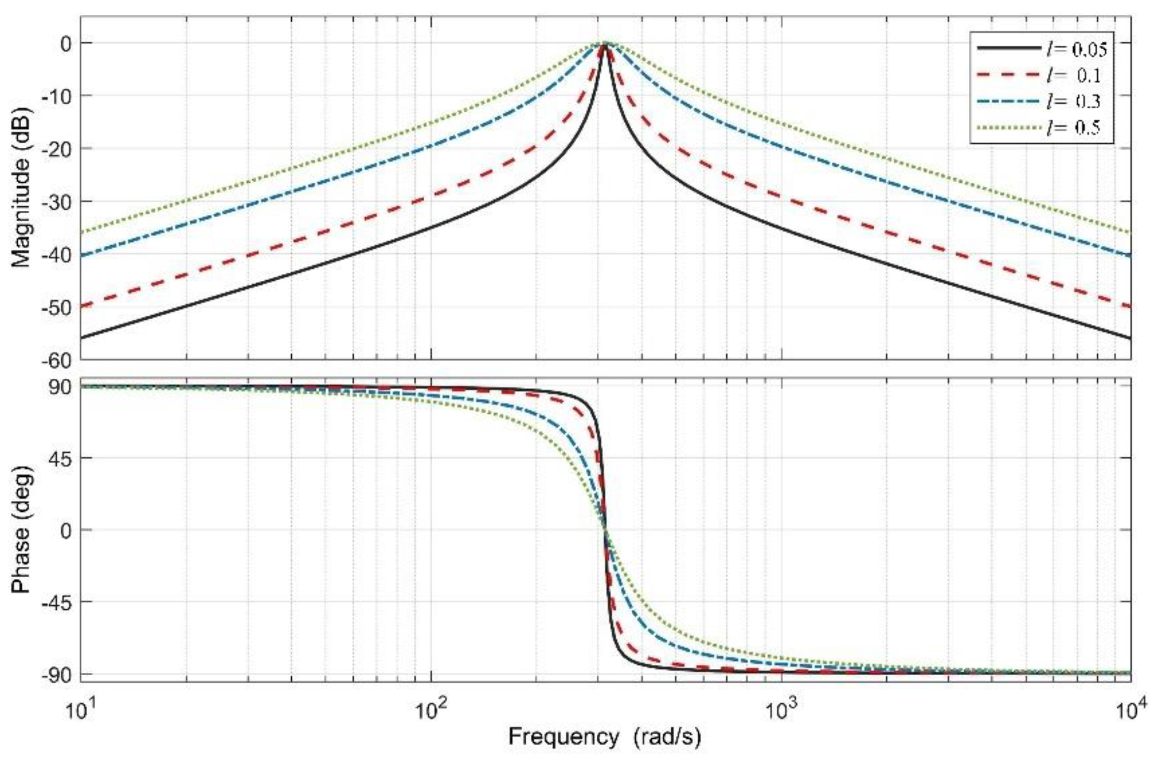
Figure 7 reveals the Bode diagrams of the SOGI transfer function $D(s)$ with l = 0.05, 0.1, 0.3, 0.5, respectively. The central frequency of SOGI in Figure 7 is 50 Hz (100π rad/s). The bandwidth of D(s) is different for different l values. As l increases from 0.05 to 0.5, the bandwidth widens, and the change of phase frequency characteristic curve also becomes slow. It can be seen that there is no delay in the phase frequency characteristic curve of D(s). Obviously, the filtering effect is better when the bandwidth is narrower, but from a practical point of view, the passband need not be too narrow.

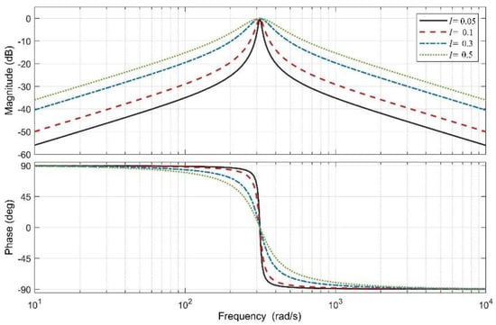
Figure 7. Bode diagram of SOGI.

When the frequency of the input signal v coincides with the center frequency of the SOGI, the output signals v′ and qv′ are two quadrature signals of the same amplitude, v′ overdetermined qv′ in phase π/2. D(s) can be considered as a second-order BPF. Let the quality factor $Q_D=1/l$, (16) can be modified as

$$D(s)=\frac{{\omega }_{\mathrm{c}}/Q_{D}s}{s^2+{\omega }_{\mathrm{c}}/Q_{D}s+{\omega }_{\mathrm{c}}{}^2}$$

(17)

As can be seen from (17), the quality factor is related to the damping factor, and the smaller the l, the better filtering performance will be, but the longer dynamic response time of the system will be, generally taking the value about $\sqrt{2}$.

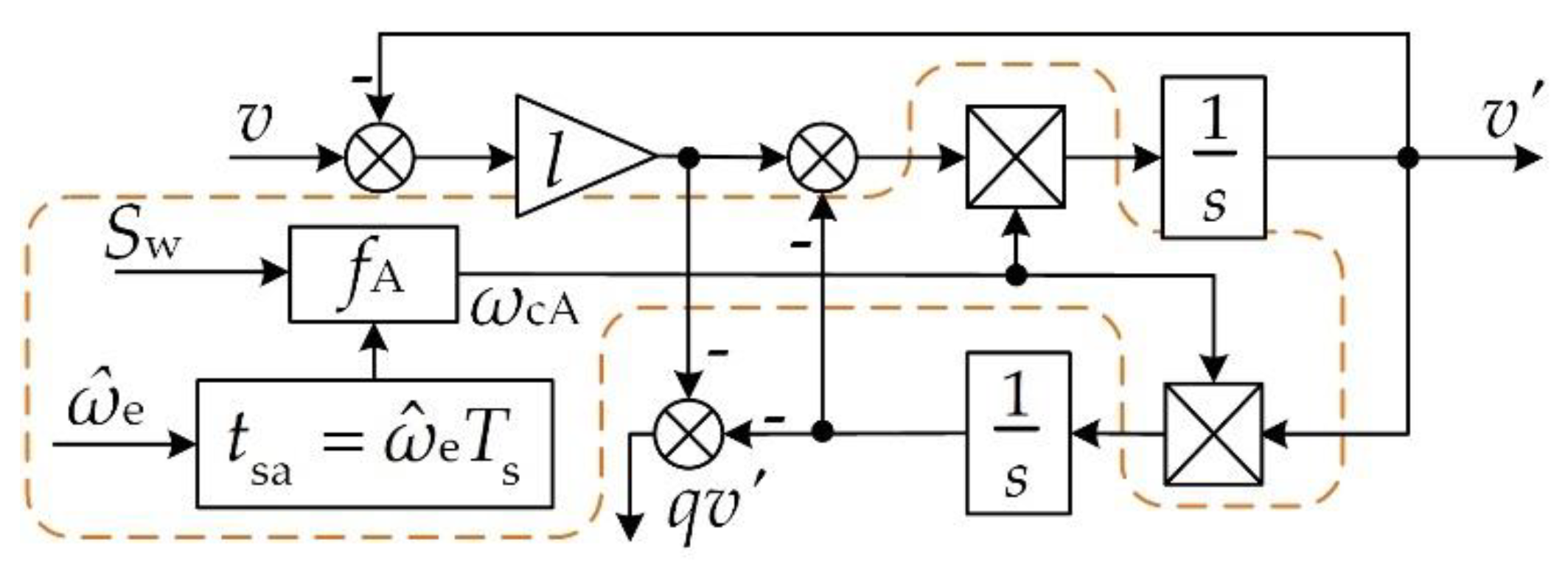
For the unstable current ripple frequency, a second-order generalized integrator with adaptive center frequency adjustment is designed, and the structure is shown in Figure 8. The switching selection frequency of the FCS-MPC controller is sampled with a sampling period of

$$t_{\mathrm{sa}}=\widehat{\omega }\mathrm{e}{T}_{\mathrm{s}}$$

(18)

where t_sa is the sampling interval time, $\widehat{\omega }\mathrm{e}$ is the estimated electro-mechanical angular velocity.

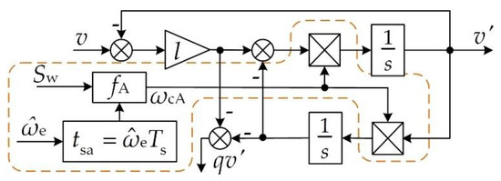
Figure 8. ASOGI structure diagram.

Due to the short sampling period, the average value of the current cycle switching times can be regarded as the current switching times, and the average switching frequency of the current cycle is

$$f_{\mathrm{A}}=\frac{S_{\mathrm{w}}}{t_{\mathrm{sa}}}$$

(19)

where S_w is the number of MPC switch selections in one cycle.

From this, the center frequency of the ASOGI-PLL can be calculated

$${\omega }_{\mathrm{cA}}=\frac{\pi S_{\mathrm{w}}}{180t_{\mathrm{sa}}}$$

(20)

As can be seen from (20), the center frequency is related to the number of switch selections and sampling interval, and the average frequency within t_sa of MPC controller operation can approximately represent the high-frequency of the current cycle. As shown in Figure 8, compared to the SOGI with a fixed center frequency, it is possible to dynamically adjust the value of the center frequency to keep it consistent with the high frequency of the current ripple. Compared with the conventional BPF, there is no phase shift, and it is able to extract the changing high frequency current ripple in FCS-MPC.

The D_A(s) transfer function of ASOGI is

$$D_{\mathrm{A}}(s)=\frac{l{\omega }_{\mathrm{cA}}s}{s^2+l{\omega }_{\mathrm{cA}}s+{\omega }_{\mathrm{cA}}{}^2}$$

(21)

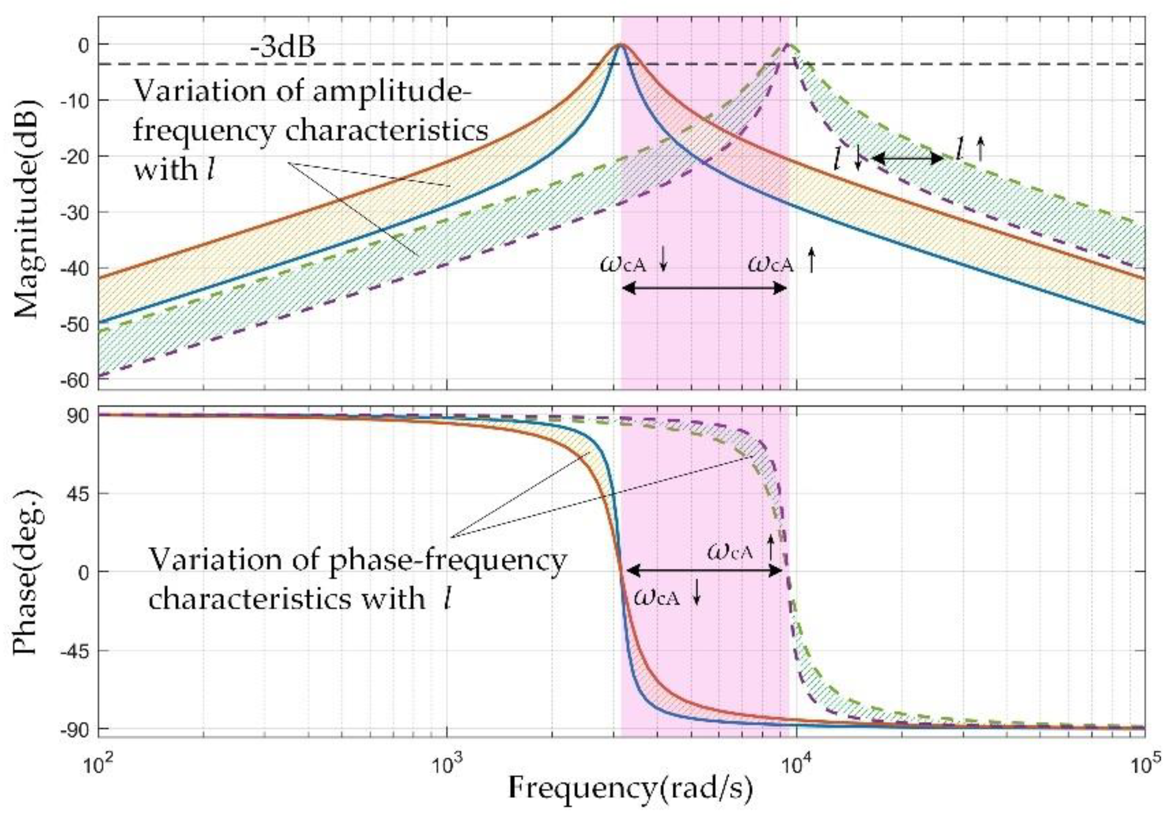
When the calculated value of ${\omega }_{\mathrm{cA}}$ is changed, the center frequency of ASOGI is also adjusted. The Bode diagrams of D_A(s) are shown in Figure 9. For different frequency input signals, ASOGI can adjust the center frequency adaptively. When ${\omega }_{\mathrm{cA}}$ is small, the amplitude-frequency characteristic curve and the phase-frequency characteristic curve of D_A(s) will be shifted to the right and conversely to the left. These actions reflect that the filter is changing the filter interval with the external signal while there is no delay in phase. When l is changed, the −3 dB bandwidth is also changed. For the universal case, 0.707 is taken, the signal frequency is generally higher in this scheme, and the value of l should be reduced appropriately.

Figure 9. Bode of D_A(s) when the center frequency changes.

Once the current passes through the ASOGI, the PLL can be used for phase locking. The structure of the composed ASOGI-PLL rotor position observer is shown in Figure 10.

Figure 10. Overall block diagram.

3.3. MPC Parameter Correction

The operating point of the motor will change due to temperature and operating condition changes, etc. Deviations between the prediction model of MPC and the actual parameters of the motor will cause parameter mismatch, resulting in inaccurate current prediction and poor control performance. As (1) and (2) show, the q-axis inductance, stator resistance R, and flux linkage ${\phi }_{\mathrm{f}}$ are critical to the performance of the MPC. In this section, Adaline is used for online identification of motor parameters and real-time correction of MPC prediction model parameters. Adaline neural network has a simple structure. It is a linear adjustable neural network with only the operations of addition, subtraction, and multiplication. The Adaline input–output relationship is expressed as

$$O(W_i,X_i)={\displaystyle \sum _{i=0}^n{W}_i{X}_i}$$

(22)

where W_i is the weight of the neural network, the weights are the identification quantities L_q, R, and ${\phi }_{\mathrm{f}}$, X_i is the input signal, d(k) is the network target input, and O(k) is the output of the network excitation function.

Adjusting network weights using least mean square (LMS)

$$\{\begin{array}{l}{W}_i(k+1)=W_i(k)+2\eta X_i\delta (k)\\ \delta (k)=d(k)-O(k)\end{array}$$

(23)

where $\eta$ is the weight adjustment factor, $\epsilon (k)$ is the error between the neural network output and the target.

When using the Adaline to identify the parameters of a motor, $\eta$ should satisfy

$$0<2\eta {\left|X(k)\right|}^2<1$$

(24)

The motor parameter identification model is constructed, and the cross-axis inductance and flux linkage are identified first. The expression of the cross-axis inductance L_q is calculated as

$$\{\begin{array}{l}{X}_{L_q}(k)=-{\omega }_{\mathrm{e}}(k)i_q(k)\\ O_{L_q}(k)=L_q(k)X_{L_q}(k)\\ d_{L_q}(k)=U_{rd}(k)-R{i}_d(k)\\ L_q(k+1)=L_q(k)+2\eta L_q{X}_{L_q}(k){\delta }_{L_q}(k)\end{array}$$

(25)

The calculated expression for flux linkage ${\phi }_{\mathrm{f}}$ is

$$\{\begin{array}{l}{X}_{{\phi }_{\mathrm{f}}}(k)={\omega }_{\mathrm{e}}(k)\\ O_{{\phi }_{\mathrm{f}}}(k)={\phi }_{\mathrm{f}}(k)X_{{\phi }_{\mathrm{f}}}(k)\\ d_{{\phi }_{\mathrm{f}}}(k)=U_{rq}(k)-{\omega }_{\mathrm{e}}(k)L_d{i}_d(k)-R{i}_q(k)\\ {\phi }_{\mathrm{f}}(k+1)={\phi }_{\mathrm{f}}(k)+2{\eta }_{{\phi }_{\mathrm{f}}}{X}_{{\phi }_{\mathrm{f}}}(k){\delta }_{{\phi }_{{}_{\mathrm{f}}}}(k)\end{array}$$

(26)

where U_rd and U_rq are the valid voltage values.

The temperature of the motor changes relatively slowly within a short period of time when the motor is started, and the resistance value does not change significantly, the calculated expression for the resistance R is

$$\{\begin{array}{l}{X}_R(k)=i_q(k)\\ O_R(k)=R(k)X_R(k)\\ d_R(k)=u_q(k)-{\phi }_{\mathrm{f}}{\omega }_{\mathrm{e}}(k)\\ R(k+1)=R(k)+2\eta X_R(k){\delta }_R(k)\end{array}$$

(27)

The overall control block diagram is shown in Figure 10.

4. Simulation and Hardware Experiments

In this section, simulation and physical platform experiments are designed and the experimental results are analyzed.

The performance of the proposed scheme was verified using a PMSM with parameters as shown in Table 2. Experiments were conducted for low speed operation, sudden variable speed, and load disturbance of the PMSM, respectively, and the experimental results were also analyzed.

Table 2. Parameters of PMSM.

Parameter	Value
Bus voltage	220 V
Pole pairs	4
Stator resistance	1.2 Ω
d-axis inductance	8.5 mH
q-axis inductance	8.5 mH
Moment of inertia	0.008 kg·m2
Permanent magnet flux	0.117 Wb
Rated speed	1500 r/min

4.1. Variable Speed Experiment at Low Speed

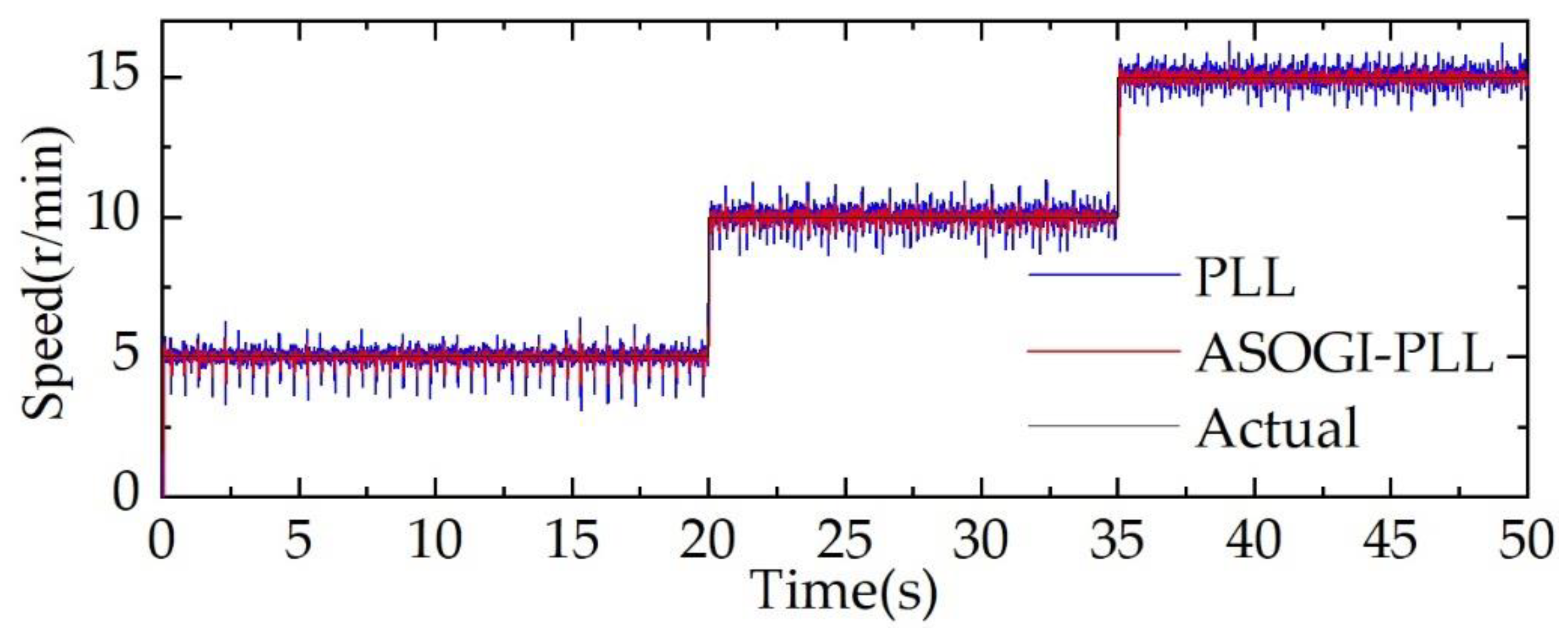
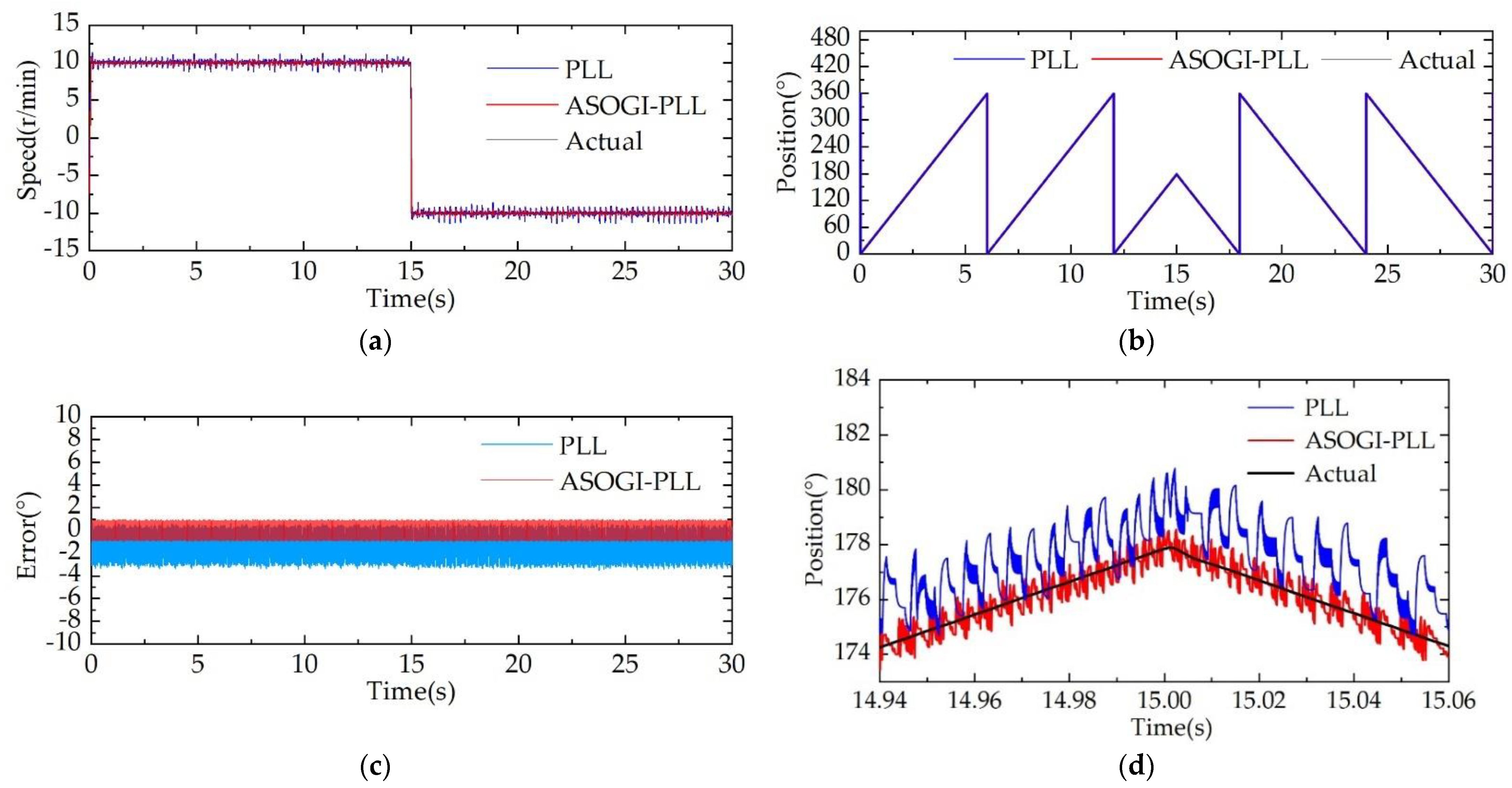
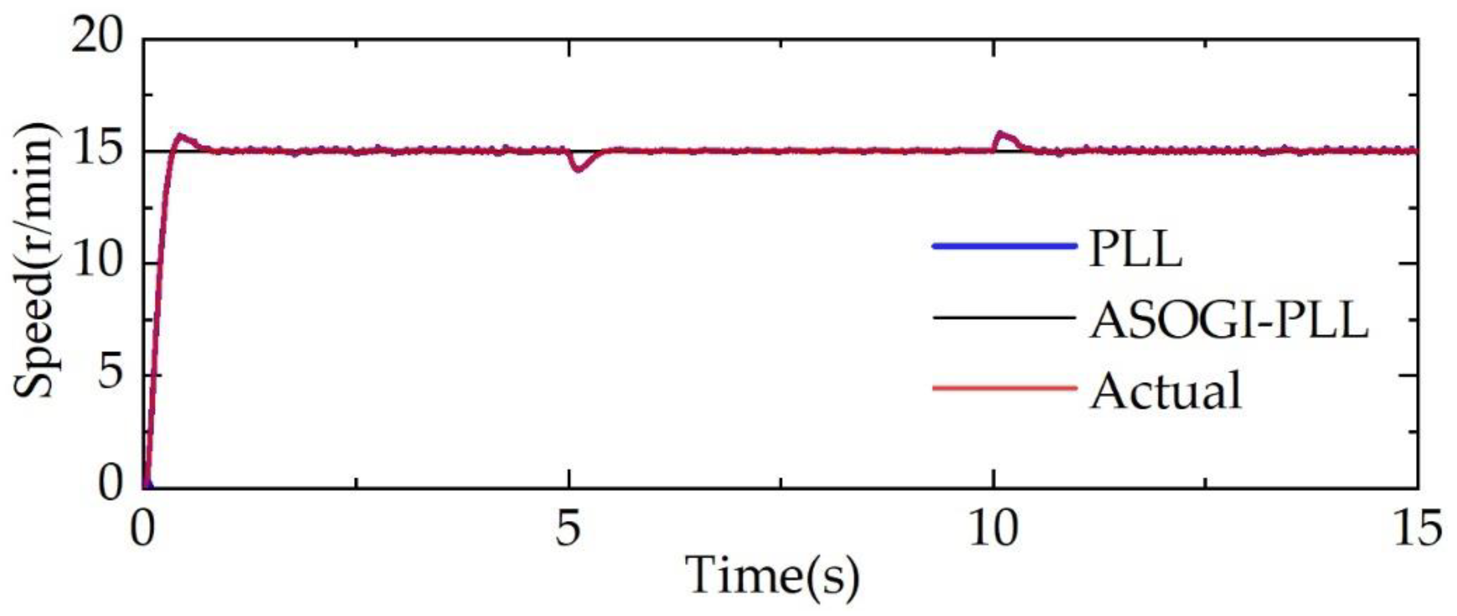
To verify the effectiveness of ASOGI-PLL for rotor position estimation at low speeds, the speed is started at a given speed of 5 r/min, the speed is increased to 10 r/min suddenly at t = 20 s, and then the speed is increased to 15 r/min suddenly after 15 s of stable operation. The speed waveform is shown in Figure 11, the speed estimation error of PLL is within 2 r/min, and the speed estimation error of ASOGI-PLL is within 1.2 r/min. The “PLL” in the legend of the experimental results refers to the BPF-PLL structure shown in Figure 5.

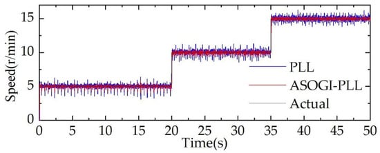
Figure 11. Speed waveform at speed up.

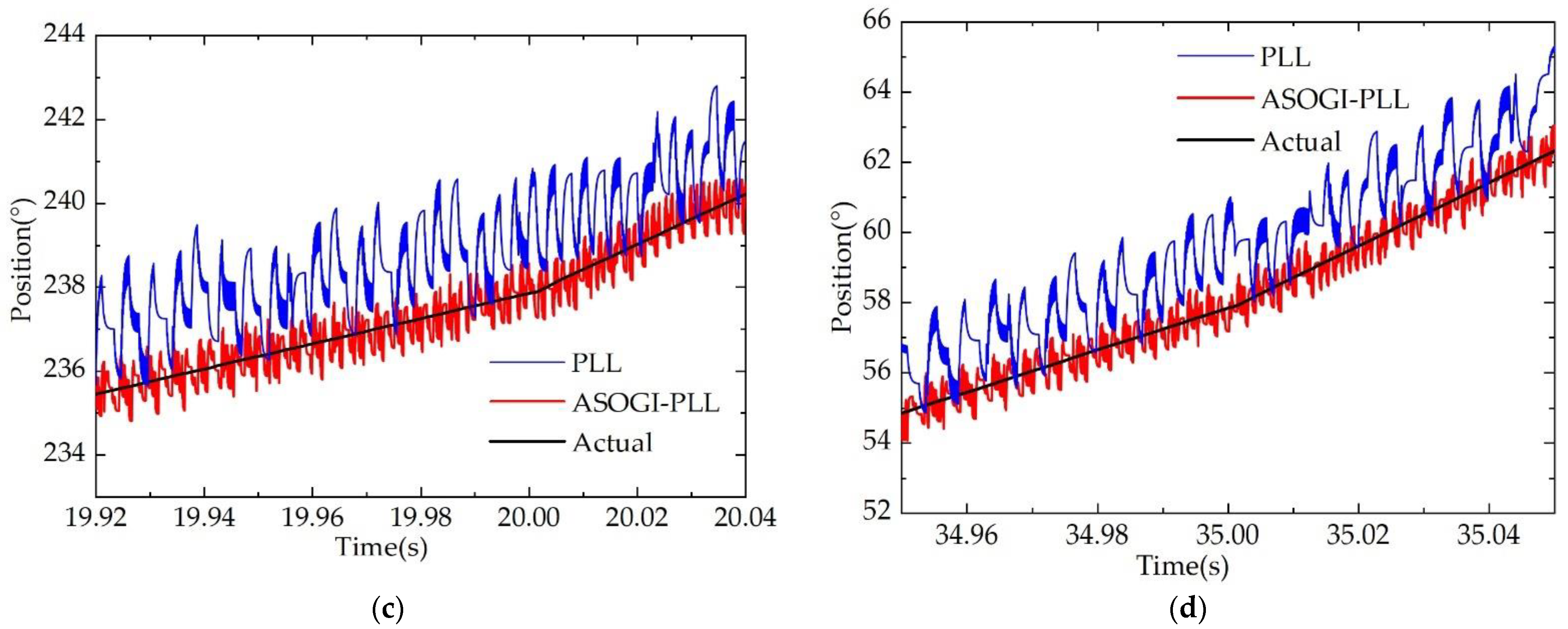
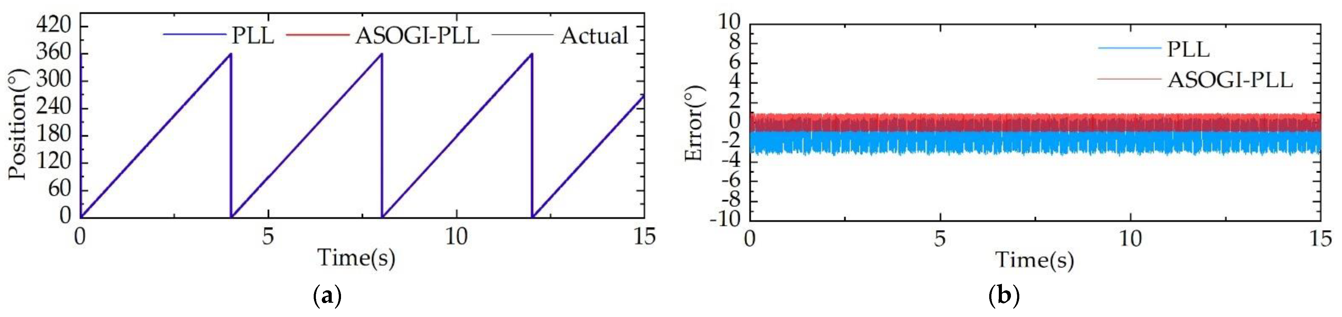
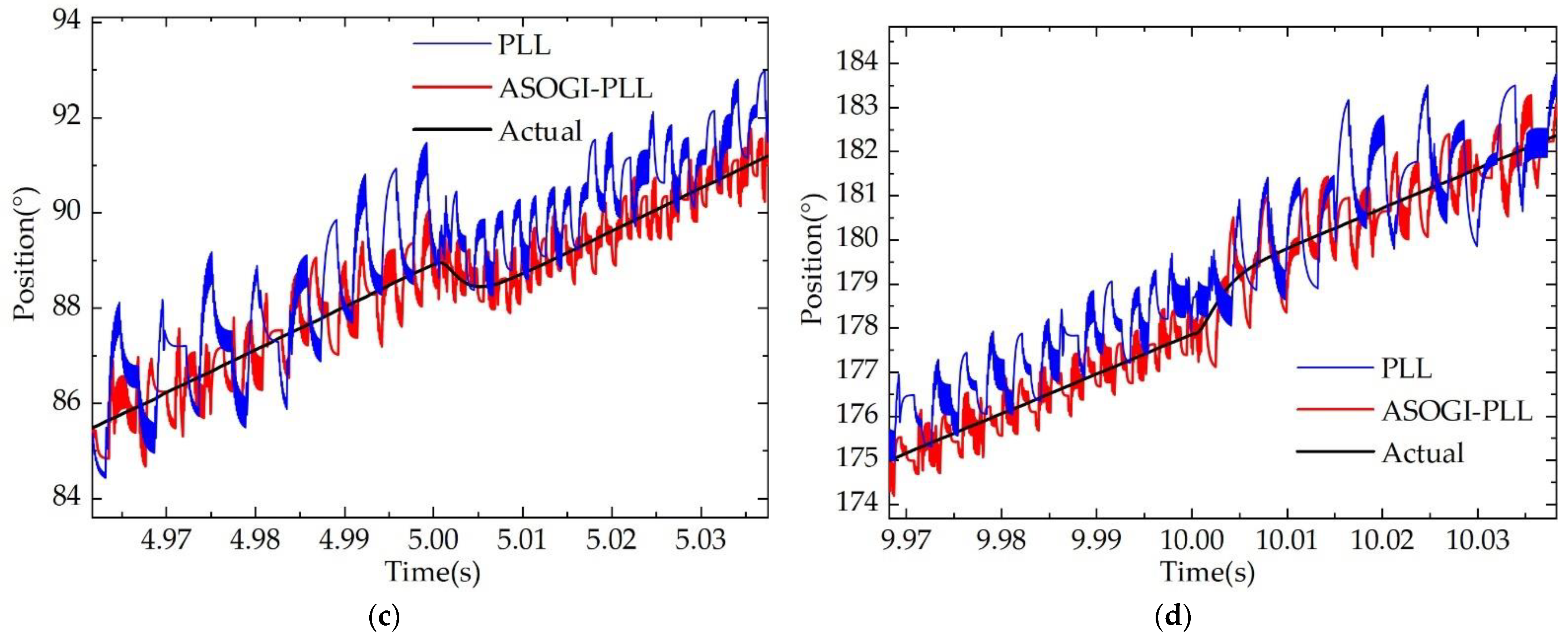
Figure 12a illustrates the rotor angle waveform during the speed change, and Figure 12b shows the rotor position estimation error. The maximum error of rotor estimation by PLL during the speed change is within 3.5° (0.06 rad), the maximum error of rotor position estimated by ASOGI-PLL is within 0.93° (0.016 rad), and the error is reduced by 73.33% relative to PLL. Figure 12c,d show the local enlargement for the speed change at t = 20 s and t = 30 s, and it can be seen that ASOGI-PLL is also able to achieve good tracking of the rotor position at the instant of speed change.

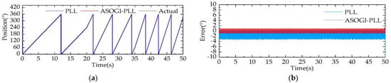
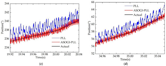
Figure 12. Speed up waveform: (a) Rotor position waveform; (b) Rotor position estimation error; (c) Rotor position local enlarged waveform at t = 20 s; (d) Rotor position local enlarged waveform at t = 35 s.

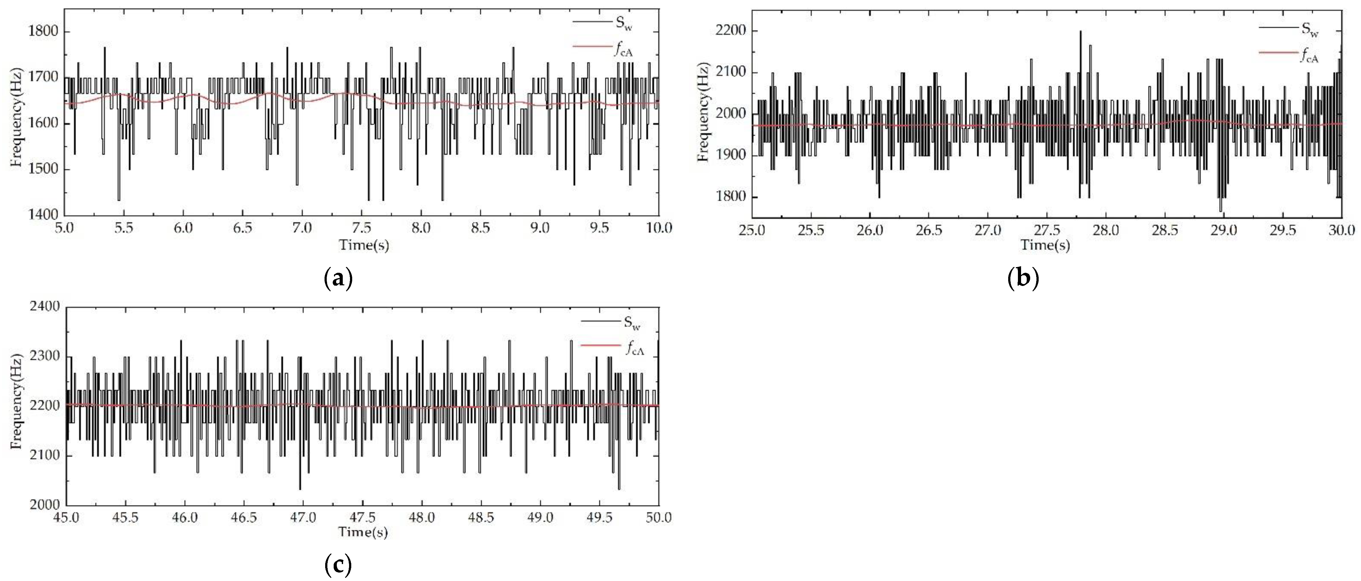
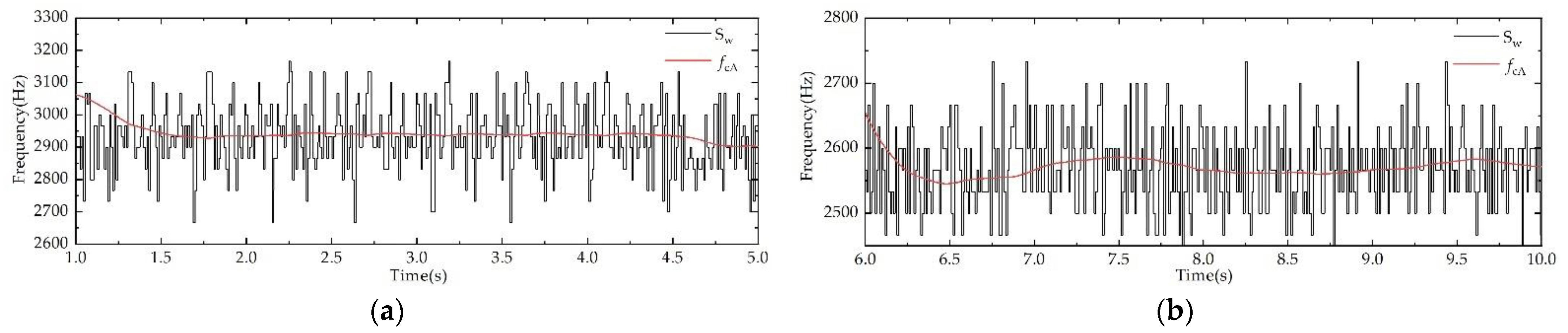
Figure 13 shows the variation of the ASOGI center frequency with the FCS-MPC switching frequency for different speeds. It is worth noting that the center frequency f_cA, obtained from the calculations in the experimental results, needs to be converted to the radian system when used for ASOGI. At different speeds, the f_cA varies with the switching frequency of the controller.

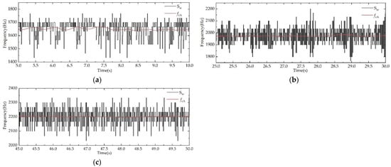
Figure 13. Switching frequency of FCS-MPC and calculated value of ASOGI center frequency: (a) At the speed of 5 r/min; (b) At the speed of 10 r/min; (c) At the speed of 15 r/min.

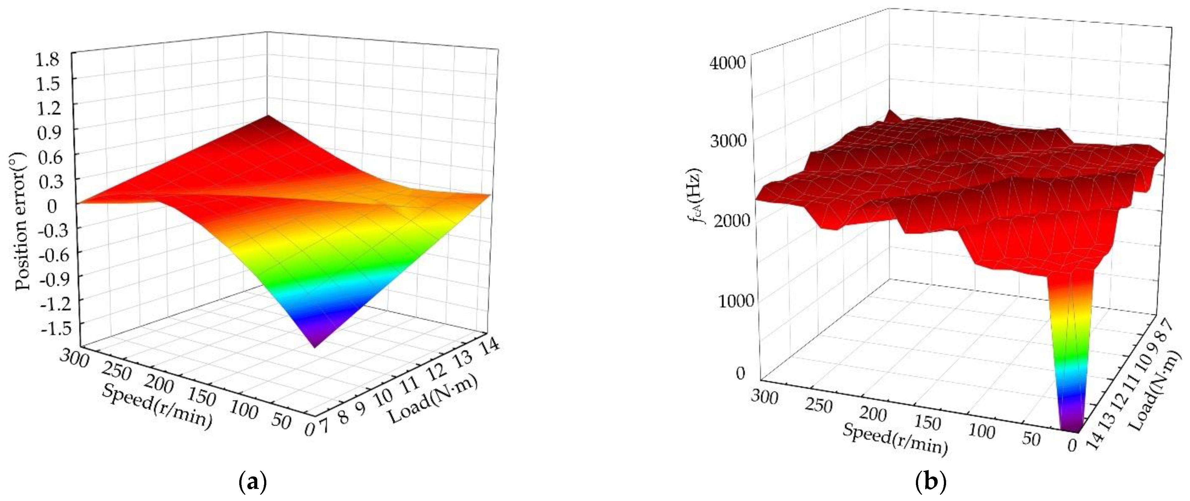
Generally, within 5% of the rated speed (75 r/min) is the ultra-low speed [31], and within 20% of the rated speed (300 r/min) is called the low speed range [32]. To test the performance of the proposed strategy in the whole low speed range, we varied the speed from 0 r/min to 300 r/min and load from 0 N·m to 14 N·m. The corresponding rotor position error changes, as shown in Figure 14a. Figure 14b shows the calculated values of the center frequency f_cA for different speeds and loads. f_cA varies with the selected frequency of the controller when the speed is stable. These show that the method has excellent performance at low speeds.

Figure 14. Results within 300 r/min: (a) Rotor position error at different speeds and loads; (b) Waveform of center frequency f_cA variation.

4.2. Motor Reversal Experiment

The motor is started at a given speed of 10 r/min under rated load, and the given speed is abruptly changed to −10 r/min at t = 15 s. The speed waveform is shown in Figure 15a, and the maximum speed estimation error is within 1.5 r/min for PLL and within 0.7 r/min for ASOGI-PLL. It converges to the stable value about 0.08 s after the speed reversal.

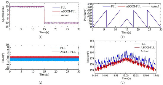
Figure 15. Rotor position waveform during motor reversal: (a) Speed waveform in reverse rotation; (b) Rotor position waveform; (c) Rotor position estimation error waveform; (d) Rotor position local enlarged waveform at t = 15 s.

The maximum error of the rotor position estimated by PLL is within 4° (0.058 rad), while the maximum error of the rotor position estimated by ASOGI-PLL is within 1.15° (0.07 rad), and the error is reduced by 71.13% compared to PLL, as shown in Figure 15b,c. Figure 15d shows the local magnified waveform of the rotor angle at the moment of reversal. The rotor angle is reversed when the motor speed is reversed, and the ASOGI-PLL is more stable than the PLL rotor position estimation.

4.3. Load Mutation Experiments

To verify the usability of the low speed control strategy under sudden load changes, the speed was started and stabilized to 15 r/min, and the load was suddenly increased from 7 N·m to 14 N·m at t = 5 s and suddenly decreased from 14 N·m to 7 N·m at t = 10 s. The speed waveform is shown in Figure 16. There is a small change in speed when the load changes, but it quickly returns to the given speed.

Figure 16. Speed waveform during sudden load change.

Figure 17a shows the rotor position waveform during sudden load change, and Figure 17b shows the rotor position error waveform. The maximum error of rotor position estimated by PLL is within 3.3° (0.058 rad), and the maximum error of rotor position estimated by ASOGI-PLL is within 0.93° (0.016 rad). Figure 17c,d shows the local enlarged view of the sudden load addition and sudden load reduction, and it can be seen that the error of rotor position estimation by ASOGI-PLL is reduced by 1.41° compared with PLL during sudden load addition and 1.33° compared with PLL during sudden load reduction. The ASOGI-PLL is able to track the rotor position accurately during sudden load changes and is more stable.

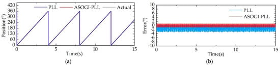
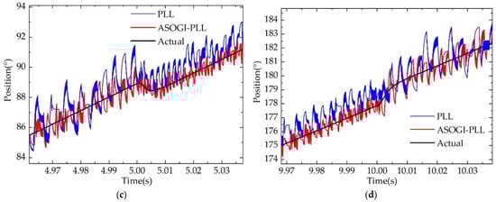
Figure 17. Sudden load change: (a) Rotor position waveform; (b) Rotor position estimation error waveform; (c) Rotor position local enlarged waveform at t = 5 s; (d) Rotor position local enlarged waveform at t = 10 s.

Figure 18 shows the variation of the ASOGI center frequency with the FCS-MPC switching frequency for different loads. At different loads, the calculated value of the center frequency varies with the selected frequency of the controller.

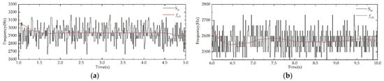
Figure 18. Switching frequency of FCS-MPC and calculated value of ASOGI center frequency: (a) At the load of 7 N·m; (b) At the load of 14 N·m.

4.4. Online Parameter Identification Experiment

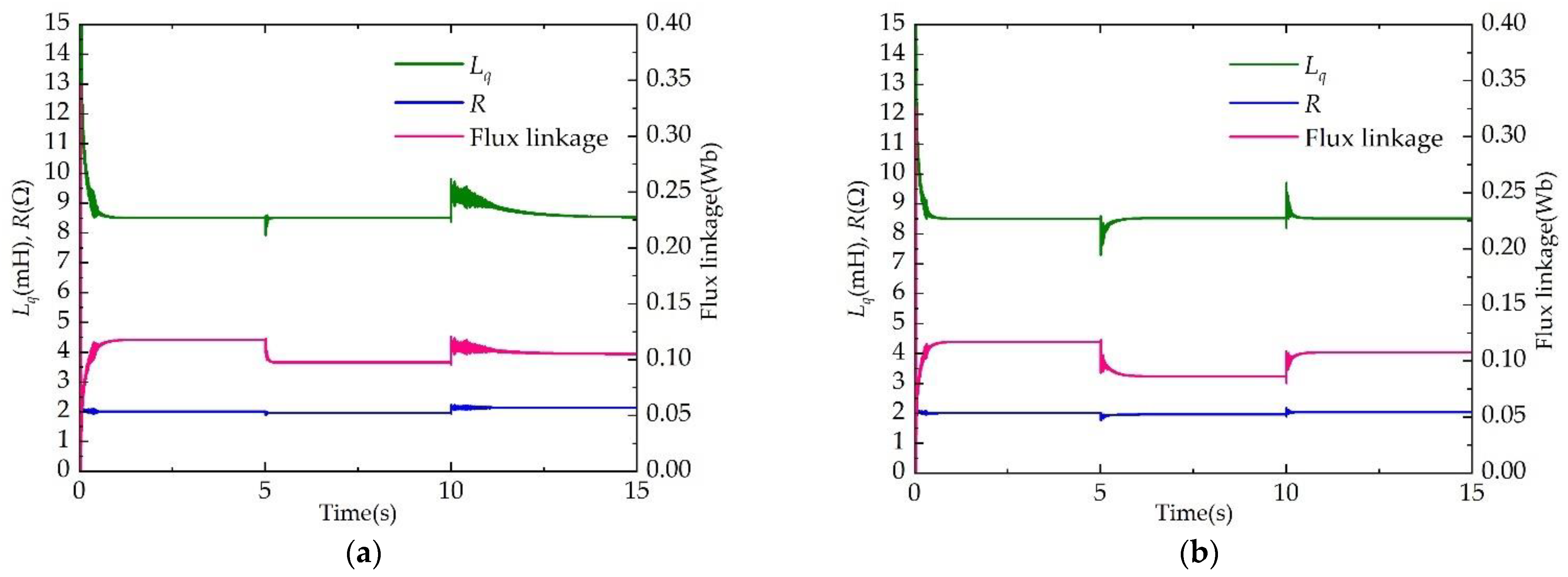
The PMSM parameters for different operating conditions were identified online using the Adaline neural network. Figure 19a shows the parameter identification results for the PMSM speed at t = 5 s with a sudden increase from 5% to 10% of the rated speed and then a sudden decrease to 5% of the rated speed at t = 10 s. The load during the speed sudden change is 50% of the rated load. The inductance and flux linkage decrease when the rotational speed increases. They increase when the rotational speed decreases. The resistance is closely related to the temperature, so the resistance value is increasing. Figure 19b shows the parameter identification results when the PMSM load increases suddenly from 50% to 100% of rated load at t = 5 s and then decreases suddenly to 50% of rated load at t = 10 s. The speed during the load sudden change experiment is 100 r/min. Both inductance and flux linkage decrease when the load increases, and they increase when the load decreases. There is an increasing trend of resistance. The Adaline neural network is accurate and fast for parameter identification under different operating conditions.

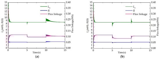
Figure 19. Parameter identification results: (a) Results of PMSM parameters identification during speed change; (b) Results of PMSM parameters identification during load change.

4.5. Hardware Experiments

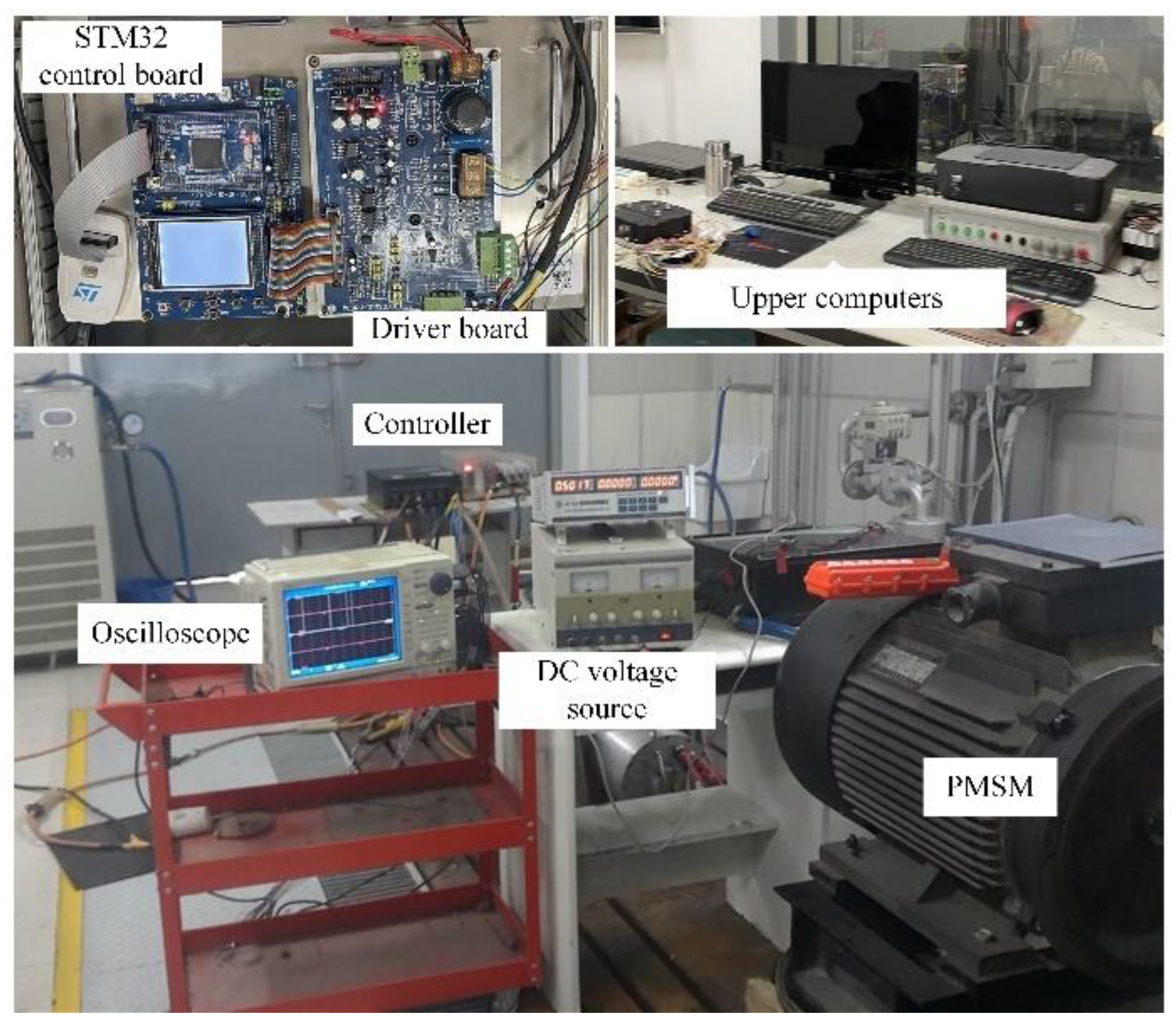
To verify the viability and effectiveness of the proposed method, an experimental platform of a 3 kW three-phase PMSM was conducted, as shown in Figure 20. The parameters of the PMSM are shown in Table 2. The control system includes an upper computer, DC power supply, ARM STM32F103, inverter, oscilloscope, PMSM, driver board, voltage sensors, and current sensor. The sampling time used in the experimental test is 1 × 10⁻⁵ s. The sampling rate of the current sensor is 10 kHz.

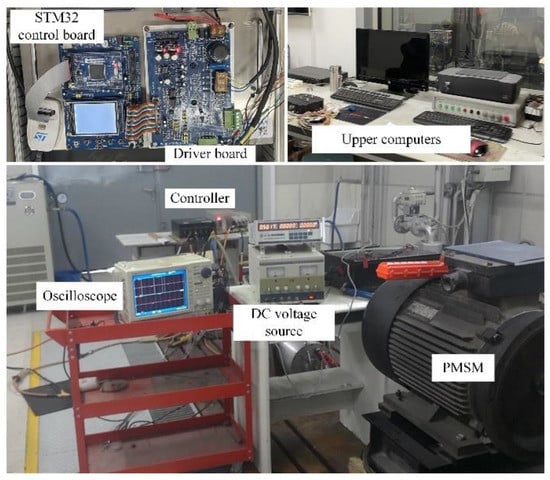
Figure 20. The experimental platform.

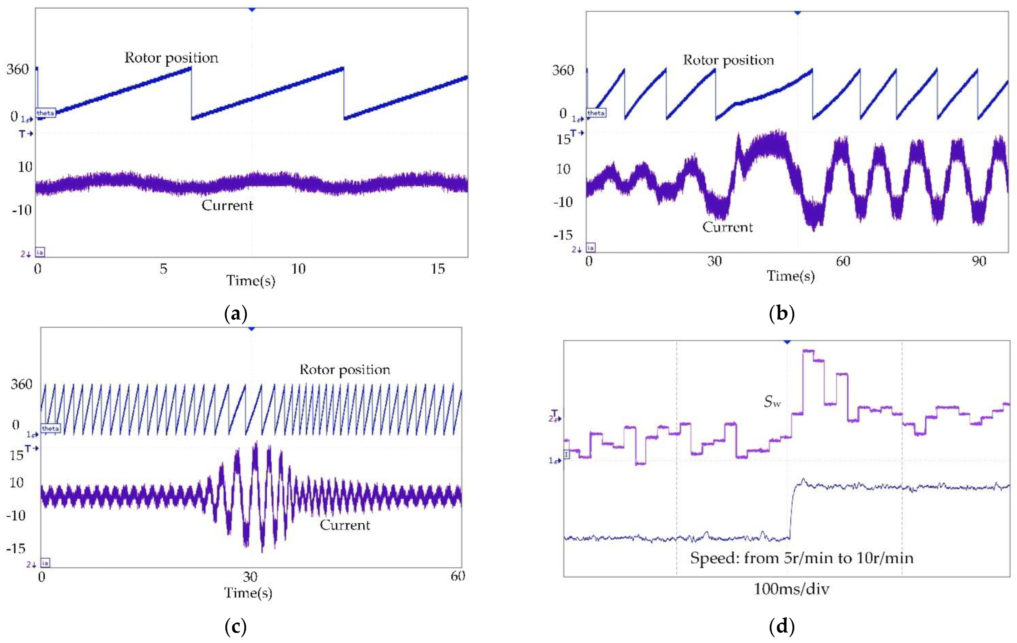
Figure 21a shows the rotor position and phase current waveforms when the PMSM is running at 10 r/min. The system operation is stable, and the rotor position is estimated accurately. Figure 21b shows the waveforms of rotor position and phase current when the load is suddenly increased. When the load increases, the current becomes larger, and the motor quickly resumes running at the given speed after a brief decrease in speed. Figure 21c shows the waveforms of rotor position and phase current when the PMSM is running at higher speed with increased load and then rapidly decreasing the load, and the system has good anti-disturbance capability and static stability. Figure 21d shows the change of the controller selection switching frequency when the speed increases. The selective switching frequency increases with the speed and load.

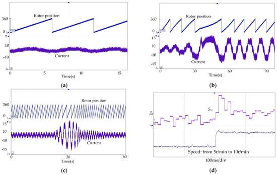
Figure 21. Hardware experimental results: (a) Rotor position and stator current at low speed; (b) Rotor position and stator current during sudden loading; (c) Rotor position and stator current during load disturbance; (d) Variation of the controller selection switching frequency when speed changes from 5 r/min to 10 r/min.

5. Conclusions

In this paper, an observer composed of ASOGI and PLL is presented to estimate the rotor position of PMSM in FCS-MPC. The inherent current ripple is generated internally by the controller, and using it instead of HFI can avoid affecting the system’s dynamic performance and reduce the system complexity. The frequency of inherent current ripple is not stable. In the proposed scheme, ASOGI is used instead of BPF, and it adjusts the center frequency adaptively according to the input signal. The irrelevant frequency signal in the high-frequency current will be filtered out by ASOGI. The ASOGI-PLL structure will estimate the rotor position accurately. PMSM parameters may change with operating conditions, and sensitive parameters can cause parameter mismatch in the controller. Adaline neural network corrects controller parameters through online parameter identification, the prediction variables will be more accurate. The experimental results demonstrate the excellent performance of the proposed scheme in the low speed or even ultra-low speed region of the PMSM.

Although this scheme has excellent position-free control performance at low PMSM speeds, the fundamental frequency has a negative impact on rotor position estimation as the speed increases, so this scheme may be limited at high speed. The strategy of combining multiple methods for different speeds may be considered more suitable for full speed high performance control of PMSM.

References

- Wang, C.-S.; Guo, C.-W.C.; Tsay, D.-M.; Perng, J.-W. PMSM Speed Control Based on Particle Swarm Optimization and Deep Deterministic Policy Gradient under Load Disturbance. Machines 2021, 9, 343. [Google Scholar] [CrossRef]
- Zhao, L.; Chen, Z.; Wang, H.; Li, L.; Mao, X.; Li, Z.; Zhang, J.; Wu, D. An Improved Deadbeat Current Controller of PMSM Based on Bilinear Discretization. Machines 2022, 10, 79. [Google Scholar] [CrossRef]
- Ma, Z.; Saeidi, S.; Kennel, R. FPGA Implementation of Model Predictive Control with Constant Switching Frequency for PMSM Drives. IEEE Trans. Ind. Informs. 2014, 10, 2055–2063. [Google Scholar] [CrossRef]
- Stellato, B.; Geyer, T.; Goulart, P.J. High-Speed Finite Control Set Model Predictive Control for Power Electronics. IEEE Trans. Power Electron. 2017, 32, 4007–4020. [Google Scholar] [CrossRef]
- Farhan, A.; Abdelrahem, M.; Hackl, C.M.; Kennel, R.; Shaltout, A.; Saleh, A. Advanced Strategy of Speed Predictive Control for Nonlinear Synchronous Reluctance Motors. Machines 2020, 8, 44. [Google Scholar] [CrossRef]
- Sun, X.; Li, T.; Yao, M.; Lei, G.; Guo, Y.; Zhu, J. Improved Finite-Control-Set Model Predictive Control with Virtual Vectors for PMSHM Drives. IEEE Trans. Energy Convers. 2021, 37, 1885–1894. [Google Scholar] [CrossRef]
- Sun, X.; Wu, M.; Lei, G.; Guo, Y.; Zhu, J. An Improved Model Predictive Current Control for PMSM Drives Based on Current Track Circle. IEEE Trans. Ind. Electron. 2020, 68, 3782–3793. [Google Scholar] [CrossRef]
- Sun, X.; Li, T.; Tian, X.; Zhu, J. Fault-Tolerant Operation of a Six-Phase Permanent Magnet Synchronous Hub Motor Based on Model Predictive Current Control with Virtual Voltage Vectors. IEEE Trans. Energy Convers. 2021, 37, 337–346. [Google Scholar] [CrossRef]
- Chen, Z.; Qiu, J.; Jin, M. Prediction-Error-Driven Position Estimation Method for Finite-Control-Set Model Predictive Control of Interior Permanent-Magnet Synchronous Motors. IEEE Trans. Emerg. Sel. Topics Power Electron. 2019, 7, 282–295. [Google Scholar] [CrossRef]
- Anayi, F.J.; Al Ibraheemi, M.M.A. Estimation of Rotor Position for Permanent Magnet Synchronous Motor at Standstill Using Sensorless Voltage Control Scheme. IEEE ASME Trans. Mechatron. 2020, 25, 1612–1621. [Google Scholar] [CrossRef]
- Morimoto, S.; Kawamoto, K.; Sanada, M.; Takeda, Y. Sensorless Control Strategy for Salient-Pole PMSM Based on Extended EMF in Rotating Reference Frame. IEEE Trans. Ind. Appl. 2002, 38, 1054–1061. [Google Scholar] [CrossRef]
- Li, H.; Zhang, X.; Yang, S.; Liu, S. Unified Graphical Model of High-Frequency Signal Injection Methods for PMSM Sensorless Control. IEEE Trans. Ind. Electron. 2020, 67, 4411–4421. [Google Scholar] [CrossRef]
- Ilioudis, V.C. Sensorless Control of Permanent Magnet Synchronous Machine with Magnetic Saliency Tracking Based on Voltage Signal Injection. Machines 2020, 8, 14. [Google Scholar] [CrossRef]
- Sun, X.; Cao, J.; Lei, G.; Guo, Y.; Zhu, J. Speed Sensorless Control for Permanent Magnet Synchronous Motors Based on Finite Position Set. IEEE Trans. Ind. Electron. 2019, 67, 6089–6100. [Google Scholar] [CrossRef]
- Liang, D.; Li, J.; Qu, R.; Kong, W. Adaptive Second-Order Sliding-Mode Observer for PMSM Sensorless Control Considering VSI Nonlinearity. IEEE Trans. Power Electron. 2018, 33, 8994–9004. [Google Scholar] [CrossRef]
- Chen, S.; Luo, Y.; Pi, Y. PMSM sensorless control with separate control strategies and smooth switch from low speed to high speed. ISA Trans. 2015, 58, 650–658. [Google Scholar] [CrossRef]
- Wang, X.; Fang, X.; Lin, S.; Lin, F.; Yang, Z. Predictive Common-Mode Voltage Suppression Method Based on Current Ripple for Permanent Magnet Synchronous Motors. IEEE Trans. Emerg. Sel. Topics Power Electron. 2019, 7, 946–955. [Google Scholar] [CrossRef]
- Rovere, L.; Formentini, A.; Gaeta, A.; Zanchetta, P.; Marchesoni, M. Sensorless Finite-Control Set Model Predictive Control for IPMSM Drives. IEEE Trans. Ind. Electron. 2016, 63, 5921–5931. [Google Scholar] [CrossRef]
- Nalakath, S.; Preindl, M.; Babak, N.M.; Emadi, A. Low speed position estimation scheme for model predictive control with finite control set. In Proceedings of the IECON 2016—42nd Annual Conference of the IEEE Industrial Electronics Society, Florence, Italy, 23–26 October 2016; pp. 2839–2844. [Google Scholar] [CrossRef]
- Nalakath, S.; Sun, Y.; Preindl, M.; Emadi, A. Optimization-Based Position Sensorless Finite Control Set Model Predictive Control for IPMSMs. IEEE Trans. Power Electron. 2018, 33, 8672–8682. [Google Scholar] [CrossRef]
- Sun, X.; Li, T.; Zhu, Z.; Lei, G.; Guo, Y.; Zhu, J. Speed Sensorless Model Predictive Current Control Based on Finite Position Set for PMSHM Drives. IEEE Trans. Transp. Electr. 2021, 7, 2743–2752. [Google Scholar] [CrossRef]
- Kumar, S.; Sreejith, R.; Singh, B. Sensorless PMSM EV Drive using Modified Enhanced PLL Based Sliding Mode Observer. In Proceedings of the International Conference on Sustainable Energy and Future Electric Transportation (SEFET), Hyderabad, India, 21–23 January 2021; pp. 1–6. [Google Scholar] [CrossRef]
- Peng, W.; Qiao, M.; Jiang, C.; Lu, X.; Zhu, X. Vibration analysis and dynamic performance improvement of high-frequency injection method. J. Power. Electron. 2021, 21, 364–375. [Google Scholar] [CrossRef]
- Tian, B.; Molinas, M.; An, Q.; Zhou, B.; Wei, J. Freewheeling Current-Based Sensorless Field-Oriented Control of Five-Phase Permanent Magnet Synchronous Motors Under Insulated Gate Bipolar Transistor Failures of a Single Phase. IEEE Trans. Ind. Electron. 2022, 69, 213–224. [Google Scholar] [CrossRef]
- Sreejith, R.; Singh, B. Sensorless Predictive Current Control of PMSM EV Drive Using DSOGI-FLL Based Sliding Mode Observer. IEEE Trans. Ind. Electron. 2021, 68, 5537–5547. [Google Scholar] [CrossRef]
- Xu, W.; Jiang, Y.; Mu, C.; Blaabjerg, F. Improved Nonlinear Flux Observer-Based Second-Order SOIFO for PMSM Sensorless Control. IEEE Trans. Power Electron. 2019, 34, 565–579. [Google Scholar] [CrossRef]
- Ahn, H.; Park, H.; Kim, C.; Lee, H. A Review of State-of-the-art Techniques for PMSM Parameter Identification. J. Electr. Eng. Technol. 2020, 15, 1177–1187. [Google Scholar] [CrossRef]
- Wang, Z.; Chai, J.; Xiang, X.; Sun, X.; Lu, H. A Novel Online Parameter Identification Algorithm Designed for Deadbeat Current Control of the Permanent-Magnet Synchronous Motor. IEEE Trans. Ind. Appl. 2022, 58, 2029–2041. [Google Scholar] [CrossRef]
- Liu, X.; Pan, Y.; Wang, L.; Xu, J.; Zhu, Y.; Li, Z. Model Predictive Control of Permanent Magnet Synchronous Motor Based on Parameter Identification and Dead Time Compensation. Prog. Electromagn. Res. C 2022, 120, 253–263. [Google Scholar] [CrossRef]
- Yu, H.; Wang, J.; Xin, Z. Model Predictive Control for PMSM Based on Discrete Space Vector Modulation with RLS Parameter Identification. Energies 2022, 15, 4041. [Google Scholar] [CrossRef]
- Wang, S.; Yang, K.; Chen, K. An Improved Position-Sensorless Control Method at Low Speed for PMSM Based on High-Frequency Signal Injection into a Rotating Reference Frame. IEEE Access 2019, 7, 86510–86521. [Google Scholar] [CrossRef]
- Gu, S.-M.; He, F.-Y.; Zhang, H. Study on Extend Kalman Filter at Low Speed in Sensor less PMSM Drives. In Proceedings of the 2009 International Conference on Electronic Computer Technology, Macau, China, 20–22 February 2009; pp. 311–316. [Google Scholar] [CrossRef]
Publisher’s Note: MDPI stays neutral with regard to jurisdictional claims in published maps and institutional affiliations. |
© 2022 by the authors. Licensee MDPI, Basel, Switzerland. This article is an open access article distributed under the terms and conditions of the Creative Commons Attribution (CC BY) license (https://creativecommons.org/licenses/by/4.0/).