Application of Kriging Model to Gear Wear Calculation under Mixed Elastohydrodynamic Lubrication

Abstract

The calculation of tooth wear under mixed elastohydrodynamic lubrication is very complex and requires consideration of many conditions such as load distribution in the tooth meshing zone, micro-convex elastoplastic deformation and tooth surface temperature. The accurate calculation of tooth wear requires a lot of time and effort. In order to calculate tooth face wear under mixed elastomeric flow lubrication quickly and accurately, a new proxy model of tooth face wear is developed using the Kriging method. The pressure distribution required for the wear calculation was obtained utilizing the modified Reynolds equation and ZMC elasto-plastic model. The numerical calculation model of gear wear was derived using the modified Archard wear model. The Kriging model was used to construct a proxy model between gear parameters and tooth wear, and the degree of approximation and goodness of fit of the Kriging model were investigated. The results are as follows. The wear depth at each position is different, the smallest at the pitch, the largest near the tooth root, and the pinion has a larger wear depth than the gear. The Kriging model is highly efficient and accurate in its computation and overcomes the shortage of excessive time spent on the calculation of numerical calculation models.

1. Introduction

Gears are widely employed in aircraft, rail transportation, marine equipment, energy machinery, and other areas as an important basic mechanical component. Tooth surface wear is a typical failure mode in heavy-duty gear systems. Tooth surface wear increases transmission error and diminishes transmission accuracy [1,2], produces vibration and noise [3,4,5], affects transmission efficiency and smoothness, and speeds up gear failure [6]. The frictional wear mechanism of heavy-duty gears and the wear calculation problem under mixed elastohydrodynamic lubrication are difficulties that must be addressed in the design, manufacture, and application of novel gears. Holm, Burwell, and Archard et al. produced consecutive adhesive wear calculation formulae, the most extensively utilized of which being Archard’s generalized wear calculation equation [7]. Flodin [8] used the single-point observation approach to compute the contact pressure and sliding velocity of gears. Lundvall et al. [9,10] applied the finite element approach to compute tooth contact pressure and sliding distance for spur gears, but the sliding distance was calculated inefficiently. Park introduced a semi-analytic contact algorithm [11] and a surface interpolation approach [12], both of which enhanced the efficiency of gear wear estimations greatly. Heavy-duty transmission systems usually operate under mixed or boundary lubrication. Johnson et al. [13] initially suggested the notion of load sharing, where the working load is thought to be carried by the lubricant film between the surface and the micro-convex under mixed elastohydrodynamic lubrication. Bearings, cams and gears often operate in a mixed lubrication condition and wear can damage the surface and affect the clearance. Sander and Allmaier et al. [14] studied the friction of a shaft diameter bearing when moving from fluid to mixed lubrication by a combination of experiments and simulations, and analyzed the effect of the limit of constant boundary coefficient and the flow factor. Sharma et al. [15] investigated the effect of wear on the mixed lubrication performance of tapered journal bearings and obtained the static and dynamic performance characteristics of the bearings under different external loads, wear depths and different taper angles. Zhang et al. [16] proposed a method to correct the rounding of the roller ends of cylindrical roller bearings using wear. The mixed lubrication model combines the average flow model with the Kogut and Etsion model for contact pressure on rough surfaces. The results show that the optimized rolls have a uniform pressure distribution and the sharp increase in contact pressure of the micro-convex disappears. Winkler et al. [17] developed a numerical simulation method for studying the wear evolution of thrust roller bearings under mixed elastohydrodynamic lubrication. During the simulation, a finite element-based three-dimensional EHL model couples the elastohydrodynamic lubrication and the microscopic surface topography. The Archard wear model, the Greenwood–Williamson load-sharing model, and the Sugimura surface adaption model are all used in the numerical simulation technique. The aforementioned models explore the wear behavior of bearings under four load situations and two distinct mineral oil types working settings. Zhu [18] analyzed the dynamics and wear characteristics of the cam and guide barrel friction pair of a gasoline engine by computer programming, and predicted the minimum oil film thickness and friction coefficient, taking into account the transient effect and mixed lubrication. It is also pointed out that the extrusion effect of the lubricant and the surface roughness of the cam and guide barrel have a significant influence on the frictional wear performance. Wu et al. [19] developed a calculation equation for gear wear that takes into account gear dynamics and elastohydrodynamic lubrication. Considering the influence of surface roughness on elastohydrodynamic lubrication, Patir and Cheng [20,21] modified the Reynolds equation proposed by Dowson [22]. Majumdar and Hamrock [23] explored the fluctuation law of the load and the oil film thickness carried by the micro-convex contact with surface roughness using the modified Reynolds equation and the rough surface contact model extended by Greenwood and Tripp [24]. Zhao et al. [25] introduced a complete rough surface contact model that accommodates elastic, plastic, and elastoplastic deformation. The model is adaptable to a large variety of loads and surface roughness values. Masjedi and Khonsari derived a numerical model for oil film thickness and micro-convex contact ratio based on Zhao’s elastic–plastic rough surface contact model [26]. They then combined the aforementioned numerical model and the theory of thermal desorption of lubricating layer to develop a computer model for the interfacial friction coefficient and wear rate under mixed lubrication [27], which they used to calculate steady-state adhesive wear of spur gear teeth [28].

In mixed elastohydrodynamic lubrication, gear wear is a progressive and cumulative process with a long time horizon to reach the limit value, and the numerical simulation step size offered by the method must not be too big to maintain acceptable accuracy. Both of these considerations make calculating the wear volume time-consuming. When a large sample size is necessary to develop the relationship between gear parameters and wear, the numerical simulation algorithm is no longer appropriate. Approximate models can be applied instead of numerical wear models to tackle the aforesaid problem. Response surface approach [29], adaptive neural network method [30], Kriging method [31], and other approximation methods are extensively utilized. The response surface approach generates a fixed form of function, which is ineffective for dealing with complicated situations. The adaptive neural network’s resilience is poor. The Kriging model, on the other hand, performs better when dealing with situations involving significant nonlinearity and abrupt local response, and it does not require a huge number of design sample points. Laurenceau et al. [32] compared the Kriging model to the response surface approach in aviation dynamics design. The Kriging model was established by Feng et al. [33] to calculate the reliability of the main shaft vibration, and the study’s findings revealed that the Kriging operation is more efficient and that the method is suitable for the reliable calculation of substantially nonlinear systems. Yang et al. [34] established the Kriging model by Latin Hypercube Sampling to solve the problem of multiple responses and implicit functions for gear trim optimization. The calculation of gear wear under mixed elastohydrodynamic lubrication involves a large number of parameters with complex relationships between them. The calculation of gear wear requires the solution of a nonlinear system of equations, which is very complex and time-consuming. Especially when a large number of wear calculations are required, such as the study of gear wear mechanism and gear transmission reliability, traditional numerical calculations cannot meet the requirements. In order to solve the above problems, this paper establishes a Kriging model for gear wear calculation under mixed elastohydrodynamic lubrication by taking advantage of the Kriging model to obtain a proxy model with high prediction accuracy and fast solution speed based on a small amount of numerical simulation results. The model is also validated.

The remainder of the paper is laid out as follows. A numerical model of tooth wear under mixed elastohydrodynamic lubrication is built in Section 2. Section 3 describes some basic theories of the Kriging method. In Section 4, the Kriging method is used to create a proxy model for tooth surface wear under mixed elastomeric lubrication, and the computational results are discussed and analyzed. Finally, Section 5 covers the main conclusions.

2. Gear Wear Model under Mixed Elastohydrodynamic Lubrication

2.1. Mixed Elastohydrodynamic Lubrication Model

In mixed elastohydrodynamic lubrication, the contact surface is a rough surface, and the Reynolds equation should be adjusted to consider surface roughness effects. The surface load is borne by the micro-convex and the oil film in mixed elastohydrodynamic lubrication issue. The surface micro-convex may be deformed elastically, elasto-plastically, or plastically when the contact surface is deformed elastically under the load. As a result, the supplementary equation utilized to express the connection between the micro-convex contact pressure and the interface gap must be solved simultaneously.

Since the tooth surface load is supplied by the oil film and the micro-convex, the sum of the oil film pressure $p_h$ and the micro-convex contact pressure $p_a$ equals the total pressure $p$, i.e.,

$$p=p_h+p_a$$

(1)

2.1.1. Governing Equations

In line-contact elastohydrodynamic lubrication, Patir and Cheng amended the Newtonian fluid steady-state Reynolds equation to include roughness effects. The equation is as follows [22]:

$$\frac{\partial }{\partial x}\left({\varnothing }_x\frac{\rho h^3}{12\mu }\frac{\partial p_h}{\partial x}\right)=u\frac{\partial \left(\rho h_T\right)}{\partial x}$$

(2)

The variables included in the above equation are the oil film thickness h, the lubricant density$\rho$, the lubricant viscosity μ, the rolling speed u, the pressure-flow coefficient ${\varnothing }_x$, and the average clearance between the contact surfaces $h_T$. Equation (2) considers the influence of fluid compressibility. The first-order ordinary differential equation of the Equation (2) can be represented as follows:

$$\frac{d{p}_h}{dx}=12\mu u\frac{\rho h_T-k_r}{{\varnothing }_x\rho h^3}$$

(3)

where $k_r$ is a constant that needs to be obtained. Substituting ${\varnothing }_x$ corresponding the isothermal surface in reference [20] to Equation (2), we obtain:

$$\frac{d{p}_h}{dx}=12\mu u\left(h_T-{\rho }^{-1}{k}_r\right)h^{-3}{\left(1-0.9e^{-0.56h/\sigma }\right)}^{-1}$$

(4)

where the surface roughness σ is defined as the standard deviation of the height of the surface micro-convex. The heights of the micro-convex on the surface obey a Gaussian distribution and the expression for $h_T$ is as follows [26]:

$$h_T=0.5h\left[1+erf\left(\frac{h}{\sqrt{2}\sigma }\right)\right]+\frac{\sigma }{\sqrt{2}\pi }exp\left(\frac{-h^2}{2{\sigma }^2}\right)$$

(5)

The density–pressure function and the viscosity–pressure function can be described as follows [26]:

$$\frac{\rho }{{\rho }_0}=1+\frac{0.6p_h}{1+1.7p_h}$$

(6)

$$\frac{\mu }{{\mu }_0}=\exp \left\{\left(\ln {\mu }_0+9.67\right)\left[-1+{\left(1+5.1\times {10}^{-9}{p}_h\right)}^Z\right]\right\}$$

(7)

where ${\rho }_0$ is the lubricant density at standard atmospheric pressure, ${\mu }_0$ is the lubricant viscosity at standard atmospheric pressure and Z is the viscosity–pressure index.

Define the following dimensionless covariates:

$$X=\frac{x}{b},H=\frac{h}{R},\overline{\mu }=\frac{\mu }{{\mu }_0},\overline{\rho }=\frac{\rho }{{\rho }_0},P_h=\frac{4R{p}_h}{E_{eff}b}=\frac{1}{E_{eff}}\sqrt{\frac{2\pi }{W}}{p}_h,U=\frac{{\mu }_0\mu }{E_{eff}R},W=\frac{w}{E_{eff}R},G=\alpha E_{eff},\overline{\sigma }=\frac{\sigma }{R}$$

(8)

The parameters above are the Hertzian contact half-width b, the effective modulus of elasticity $E_{eff}$ ($E_{eff}=2E_{eq}$), the equivalent radius R, and the load w. In dimensionless form, the Reynolds equation and load balance equation may be expressed as:

$$\frac{d{P}_h}{dX}=48\overline{\mu }U\left(H_T-{\overline{\rho }}^{-1}{K}_r\right)H^{-3}{\left(1-0.9e^{-0.56H/\overline{\sigma }}\right)}^{-1}$$

(9)

$$\frac{\pi }{2}={{\displaystyle \int }}_{X_{min}}^{X_{end}}{P}_h\left(X\right)dX+{{\displaystyle \int }}_{X_{min}}^{X_{end}}{P}_a\left(X\right)dX$$

(10)

where $X_{min}$ and $X_{end}$ are the entrance and exit locations. Considering the elastic deformation and contact deformation of the surface, the expression for the lubricant film is [26]:

$$h\left(x\right)=h_0+\frac{x^2}{2R}-\frac{2}{\pi E_{eff}}{{\displaystyle \int }}_{x_{min}}^{x_{end}}p\ln {\left(x-s\right)}^{2}ds$$

(11)

where $h_0$ is a constant which is related to the total pressure p. The dimensionless form is given by:

$$H\left(X\right)=H_{00}+\frac{4W}{\pi }\left[X^2-\frac{1}{\pi }{{\displaystyle \int }}_{X_{min}}^{X_{end}}P\ln {\left(X-S\right)}^{2}dS\right]$$

(12)

2.1.2. Rough Surface Pressure Distribution Function

The rough surface contact pressure is the contact pressure between micro-convexes, which must account for both elastic, elastic–plastic, and completely plastic deformation of the micro-convex contact. Zhao’s elastic–plastic rough surface contact model [25] is applied to derive a pressure distribution function on the rough surface:

$$\overline{\beta }=\frac{\beta }{R},\overline{n}=n{R}^2,V=\frac{hd}{E_{eff}}$$

(13)

$$\begin{array}{cc}{P}_a=\frac{4R}{E_{eff}b}{p}_a=& \frac{2}{3}\overline{n}{\overline{\beta }}^{0.5}{\overline{\sigma }}^{1.5}{W}^{-0.5}\left(\frac{\overline{\sigma }}{{\overline{\sigma }}_s}\right){{\displaystyle \int }}_{I_1}^{I_2}{\left(z^{*}-I_1\right)}^{1.5}{e}^{-0.5{\left(\frac{\overline{\sigma }}{{\overline{\sigma }}_s}{z}^{*}\right)}^2}d{z}^{*}\hfill \\ & +2\pi V\overline{n}\overline{\beta }\overline{\sigma }{W}^{-0.5}\left(\frac{\overline{\sigma }}{{\overline{\sigma }}_s}\right){{\displaystyle \int }}_{I_3}^{\infty }\left(z^{*}-I_1\right)e^{-0.5{\left(\frac{\overline{\sigma }}{{\overline{\sigma }}_s}{z}^{*}\right)}^2}d{z}^{*}\hfill \\ & +\pi V\overline{n}\overline{\beta }\overline{\sigma }{W}^{-0.5}\left(\frac{\overline{\sigma }}{{\overline{\sigma }}_s}\right){{\displaystyle \int }}_{I_2}^{I_3}\left(z^{*}-I_1\right)e^{-0.5{\left(\frac{\overline{\sigma }}{{\overline{\sigma }}_s}{z}^{*}\right)}^2}\hfill \\ & \times \left[1-0.6\frac{\ln {\overline{w}}_2-\ln \left(z^{*}-I_1\right)}{\ln {\overline{w}}_2-\ln {\overline{w}}_1}\right]\hfill \\ & \times \left\{1-2{\left[\frac{\left(z^{*}-I_1\right)-{\overline{w}}_1}{{\overline{w}}_2-{\overline{w}}_1}\right]}^3+3{\left[\frac{\left(z^{*}-I_1\right)-{\overline{w}}_1}{{\overline{w}}_2-{\overline{w}}_1}\right]}^2\right\}d{z}^{*}\hfill \end{array}$$

(14)

where

$$I_1=\frac{H-{\overline{y}}_s}{\overline{\sigma }},I_2=\frac{H-{\overline{y}}_s+{\overline{w}}_1}{\overline{\sigma }},I_3=\frac{H-{\overline{y}}_s+{\overline{w}}_2}{\overline{\sigma }},{\overline{\sigma }}_s=\frac{{\sigma }_s}{R},{\overline{y}}_s=\frac{y_s}{R},{\overline{w}}_1={\left(0.6\pi V\right)}^2\overline{\beta }$$

(15)

Furthermore, ${\overline{w}}_2=54{\overline{w}}_1$. Since $\overline{n}\overline{\beta }\overline{\sigma }=n\beta \sigma$, either of these input parameters can be represented by the other parameters. The micro-convex density can be described by the following function:

$$\overline{n}=0.05/\left(\overline{\beta }\overline{\sigma }\right)$$

(16)

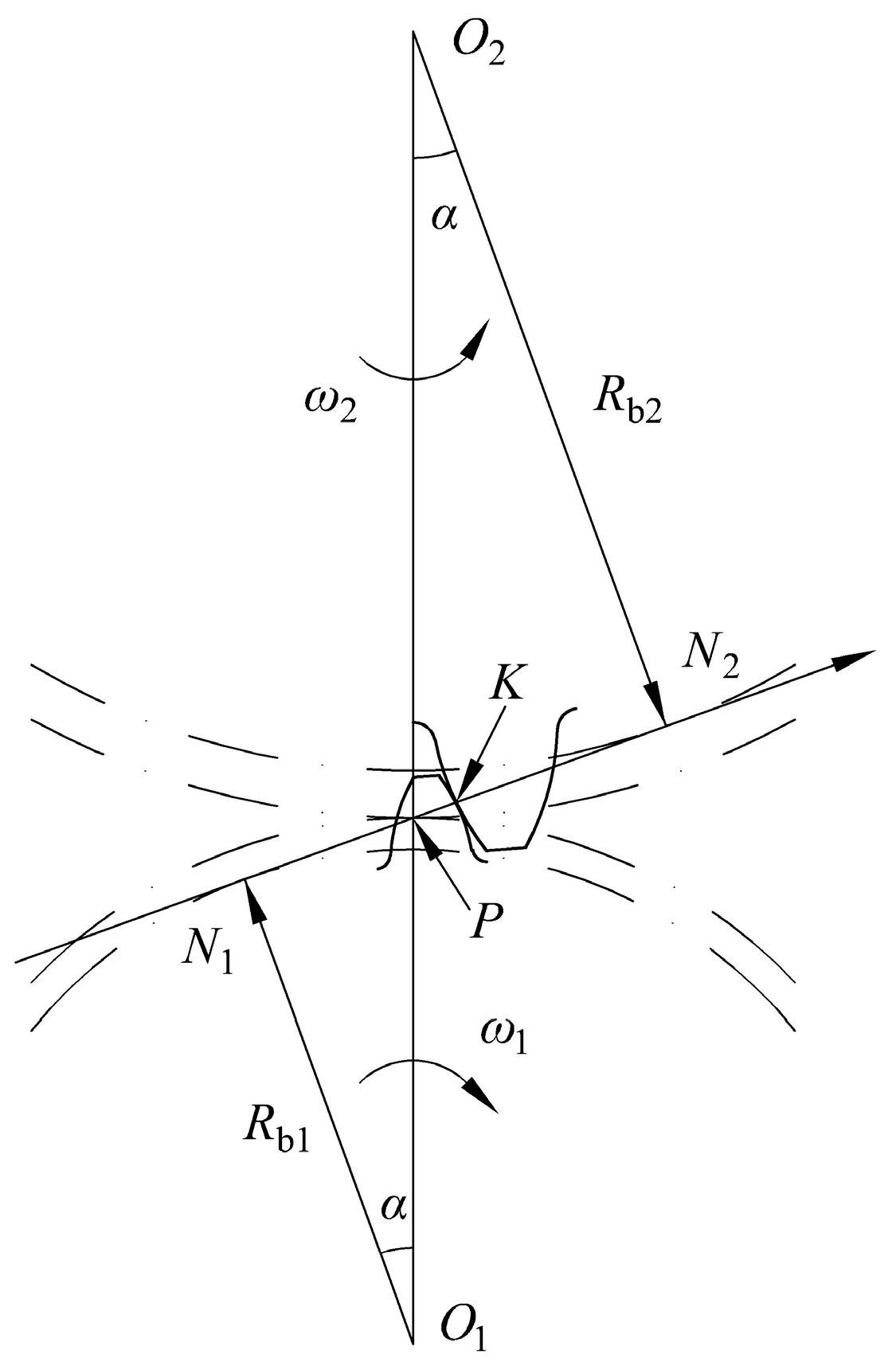
2.2. Geometry and Kinematics

The tooth profile of a spur gear is involute. The gear meshing relationship is shown in Figure 1.

The curvature radius of the pinion is $R_1$ and the curvature radius of the gear is $R_2$. They can be obtained by the radii of the pinion and gear pitch circle $R_{\mathrm{b}1}$, $R_{\mathrm{b}2}$:

$$\{\begin{array}{c}{R}_1=R_{\mathrm{b}1}\sin \alpha +y\\ R_2=R_{\mathrm{b}2}\sin \alpha -y\end{array}$$

(17)

where y is the distance from the current meshing point to the pitch on the meshing line. The linear velocities at the meshing point are:

$$\{\begin{array}{c}{u}_1=\pi n_1{R}_1/30\\ u_2=\pi n_2{R}_2/30\end{array}$$

(18)

The linear velocities of the pinion and gear are $u_1$, $u_2$. The rotational speeds are $n_1$, $n_2$. The sliding distances of the pinion and gear are $s_1$, $s_2$ which can be estimated according to the following formula:

$$\{\begin{array}{c}{s}_1=2a_H\frac{\left|u_1-u_2\right|}{u_1}\\ s_2=2a_H\frac{\left|u_1-u_2\right|}{u_2}\end{array}$$

(19)

where $a_H$ is the contact half-width and can be obtained by the following function:

$$a_H=\sqrt{\frac{4F·R}{\pi ·E_{eq}}}$$

(20)

2.3. Wear Model

A model for calculating the wear rate under mixed lubrication is derived on the basis of the Archard wear model [27]:

$${\Omega }_{lub}=K\Psi \left(\frac{L_a}{100}\right)\frac{F{u}_s}{v}$$

(21)

where ${\Omega }_{lub}$ is the volume wear rate under the lubricated condition, $L_a$ is the surface micro-convex contact ratio, F is the contact load, $u_s$ is the relative sliding velocity, Ψ is the oil film deficit coefficient, and the expression is as follows:

$$\Psi =1-exp\left[-\frac{X}{u_s{t}_0}exp\left(\frac{E_a}{R_g{T}_s}\right)\right]$$

(22)

where X is the diameter of the lubricant molecule, $t_0$ is the basic time of molecular vibration in the adsorption state, $E_a$ is the heat of adsorption of the lubricant at the interface, $R_g$ is the molar gas constant, and $T_s$ is the interface flash temperature. Based on the flash temperature theory of Tian and Kennedy [35], the formula of the tooth surface flash temperature is:

$$T_S=T_0+\Delta T$$

(23)

$$\Delta T=\frac{2a_{H}q}{\sqrt{\pi }\left(K_1\sqrt{1+P_{e1}}+K_2\sqrt{1+P_{e2}}\right)}$$

(24)

$$q=f_c{u}_{s}p\left(L_a/100\right)+u_s{\Lambda }_{lim}p\left(1-L_a/100\right)$$

(25)

where $K_1$, $K_2$ are the thermal conductivities of the two contact surfaces, q is the average heat generated at the contact point, $P_{e1}$, $P_{e2}$ are the Peclet coefficients of the two contact surfaces, ${\Lambda }_{lim}$ is the ultimate shear stress coefficient, and $f_c$ is the micro-convex friction coefficient.

Noting that $p=F/A$ and ${\Omega }_{lub}=Ah$, A is the contact area, we can obtain the rate of wear depth to sliding distance as shown in the following equation:

$$\frac{h}{u_s}=K\Psi \left(\frac{L_a}{100}\right)\frac{p}{v}$$

(26)

Therefore, the wear depth of the gear after $n_0$ revolutions can be expressed as:

$$h={\displaystyle \sum }_{n=1}^{n_0}K\Psi \left(\frac{L_a}{100}\right)\frac{p}{v}s$$

(27)

The cumulative wear of gears is minor when the number of engagements is low, and the geometry and pressure distribution of the tooth surface can be estimated to remain constant. The contact parameters must be updated when the number of meshes is large enough and the cumulative wear reaches a certain level.

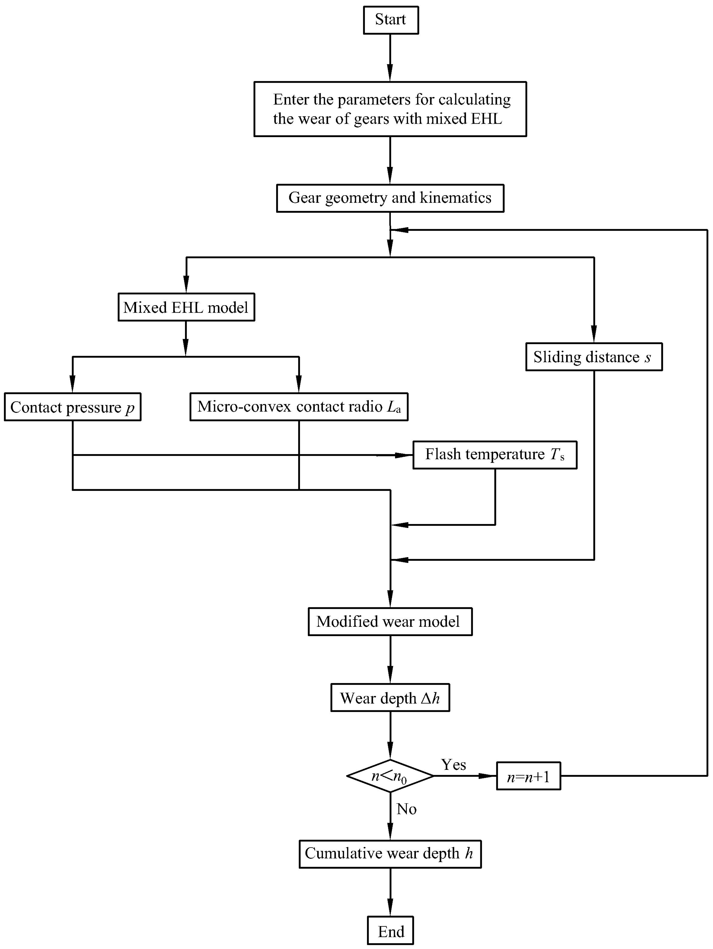
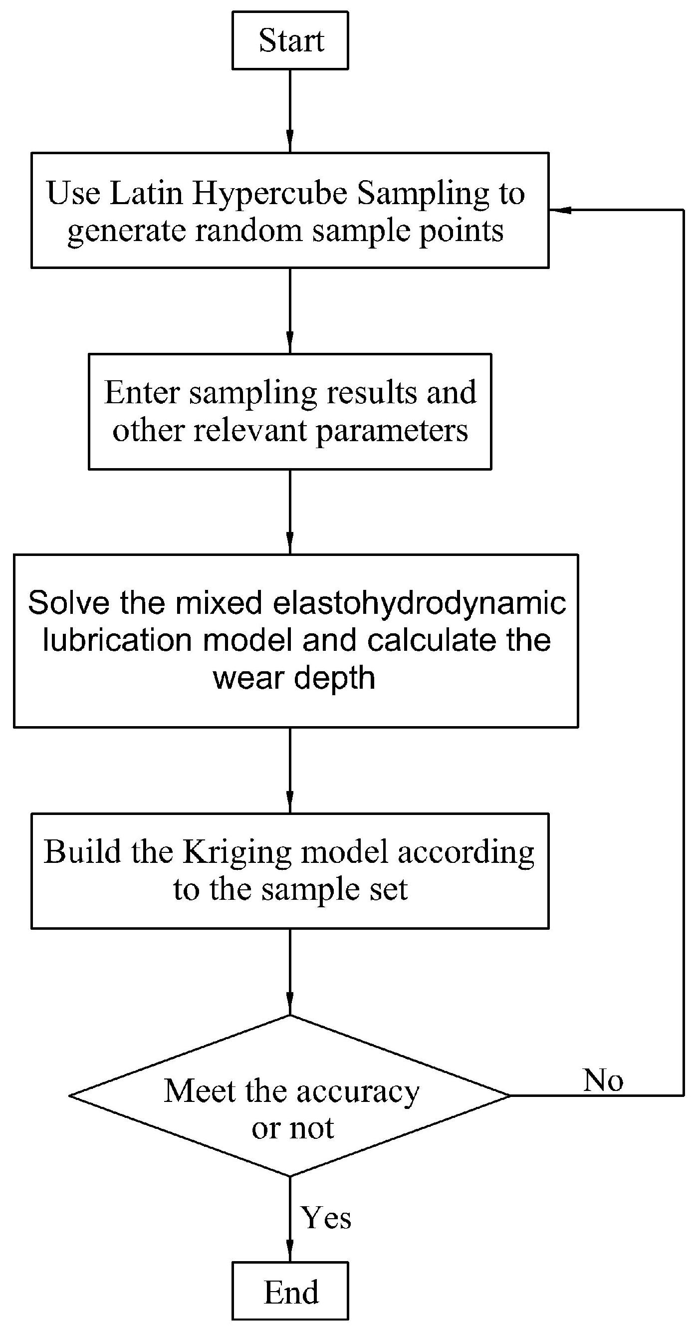
2.4. Numerical Procedure

The Newton–Raphson algorithm is used to solve for the pressure and oil film thickness after the Equations (9), (10), (12) and (14) are discretized using the finite difference approach. The boundary conditions are $X_{min}=-4$ at the inlet and the outlet location at several nodes after $X=1$. At each node, the film thickness and micro-convex contact pressure are determined. After forming the Jacobi matrix, the film pressure, $K_r$, and $H_{00}$ at each node are obtained by solving the system of equations. The new value of the total pressure is used to update the film thickness, and iterations are repeated until the results converge. The contact pressure, micro-convex contact ratio and gear sliding distance, as well as other parameters, are imported into the modified Archard wear model for the calculation of the wear depth. Each wear cycle includes 1000 revolutions of the pinion.

It should be noted that the steady-state infinite line contact elastohydrodynamic lubrication model is established in this paper. In involute spur gear elastohydrodynamic lubrication, the calculation of the finite line contact model is very close to that of the infinite line contact model, thus the infinite line contact model is chosen to simplify the calculation in this paper. In the 2D case, we may expand the minimum lubricant gap, so the wear will be larger outside the $\mathrm{y}=0$ plane. Since the load and contact radius of curvature varies with time, leading to a damping effect of the lubricant during the film thickness change, the calculated value of the film thickness may be slightly lower in this model because the time-varying effect is not considered, resulting in a higher wear depth of the gear. In addition, the model ignores the effects of non-Newtonian rheological properties of the fluid and thermal effects on the film thickness.

The specific calculation process is shown in Figure 2.

3. Kriging Model

The Kriging model is a semi-parametric difference model that does not need the state function to be specified in any particular manner. Compared to numerical calculations, the model of response and model parameters built by the Kriging method can quickly and accurately predict the response values when given a sample [36]. The Kriging model is expressed as:

$$G\left(x\right)={\displaystyle \sum }_{h=1}^p{\beta }_h{g}_h\left(x\right)+z\left(x\right)=g^T\left(x\right)\beta +z\left(x\right)$$

(28)

where $g^T\left(x\right)\beta$ is the regression model, β is the regression coefficient and g(x) is the polynomial function of the random variable x. z(x) is the stochastic process function, reflecting the approximation of the local deviation, which has a mean of 0 and variance ${\sigma }^2$, and its covariance matrix is

$$\mathrm{Cov}\left[z\left(x_i\right),z\left(x_j\right)\right]={\sigma }^{2}R\left(x_i,x_j;\theta \right)$$

(29)

where $R\left(x_i,x_j;\theta \right)$ is the correlation function which is usually expressed by the Gaussian correlation equation:

$$R\left(x_i,x_j;\theta \right)={\displaystyle \prod }_{m=1}^{M}exp\left[-{\theta }_m{\left(x_i^m-x_j^m\right)}^2\right]$$

(30)

where $x_i{}^m$ is the mth component of the sample point $x_i$.

Given a set of training samples $S=\left[x_1,x_2,···,x_N\right]$, the response values are calculated according to the corresponding real functional functions and expressed in vector form as $Y={\left[g(x_{1)},g\left(x_2\right),···,g\left(x_N\right)\right]}^T$, the unknown parameters $\beta$, ${\sigma }^2$ can be estimated by maximum likelihood estimation:

$$\widehat{\beta }={\left(G^T{R}^{-1}G\right)}^{-1}{G}^T{R}^{-1}Y$$

(31)

$${\widehat{\sigma }}^2=\frac{1}{N}{\left(Y-G^T\beta \right)}^T{R}^{-1}\left(Y-G^T\beta \right)$$

(32)

$$G={\left[g\left(x_1\right),g\left(x_2\right),···,g\left(x_N\right)\right]}^T$$

(33)

Applying the Kriging model, the predicted response value of the point x to be measured is obtained as:

$$\widehat{G}\left(x\right)=g\left(x\right)\widehat{\beta }+r{\left(x\right)}^T\gamma$$

(34)

$${\sigma }_{G\left(x\right)}^2={\widehat{\sigma }}^2\left[1+u^T\left(x\right){\left(G^T{R}^{-1}G\right)}^{-1}u\left(x\right)-r^T\left(x\right)R^{-1}r\left(x\right)\right]$$

(35)

$$R={\left(R\left(x_i,x_j;\theta \right)\right)}_{N\times N}$$

(36)

$$\mathsf{\gamma }=R^{-1}\left(Y-G\widehat{\beta }\right)$$

(37)

$$r\left(x\right)={\left[R\left(x_1,x;\theta \right),···,R\left(x_N,x;\theta \right)\right]}^T$$

(38)

$$u\left(x\right)=G^T{R}^{-1}r\left(x\right)-g\left(x\right)$$

(39)

The training random sample points, denoted by S, are generated by the Latin Hypercube Sampling method, and their actual functional response values, denoted by Y, need to be calculated by calculation. Using the training sample points S and the actual functional response value Y, the Kriging model is built. The Kriging model’s regression model is the main polynomial, with a Gaussian correlation function as the correlation function. The flowchart for constructing the gear wear Kriging model under mixed elastohydrodynamic lubrication is shown in Figure 3. The input values of the Kriging model are W, U, G, $\overline{\sigma }$, $\overline{\beta }$, V and wear time t. By taking the time parameter into account in the Kriging model, the wear trend can be predicted quickly and accurately. The output value of the model is the wear depth of gears.

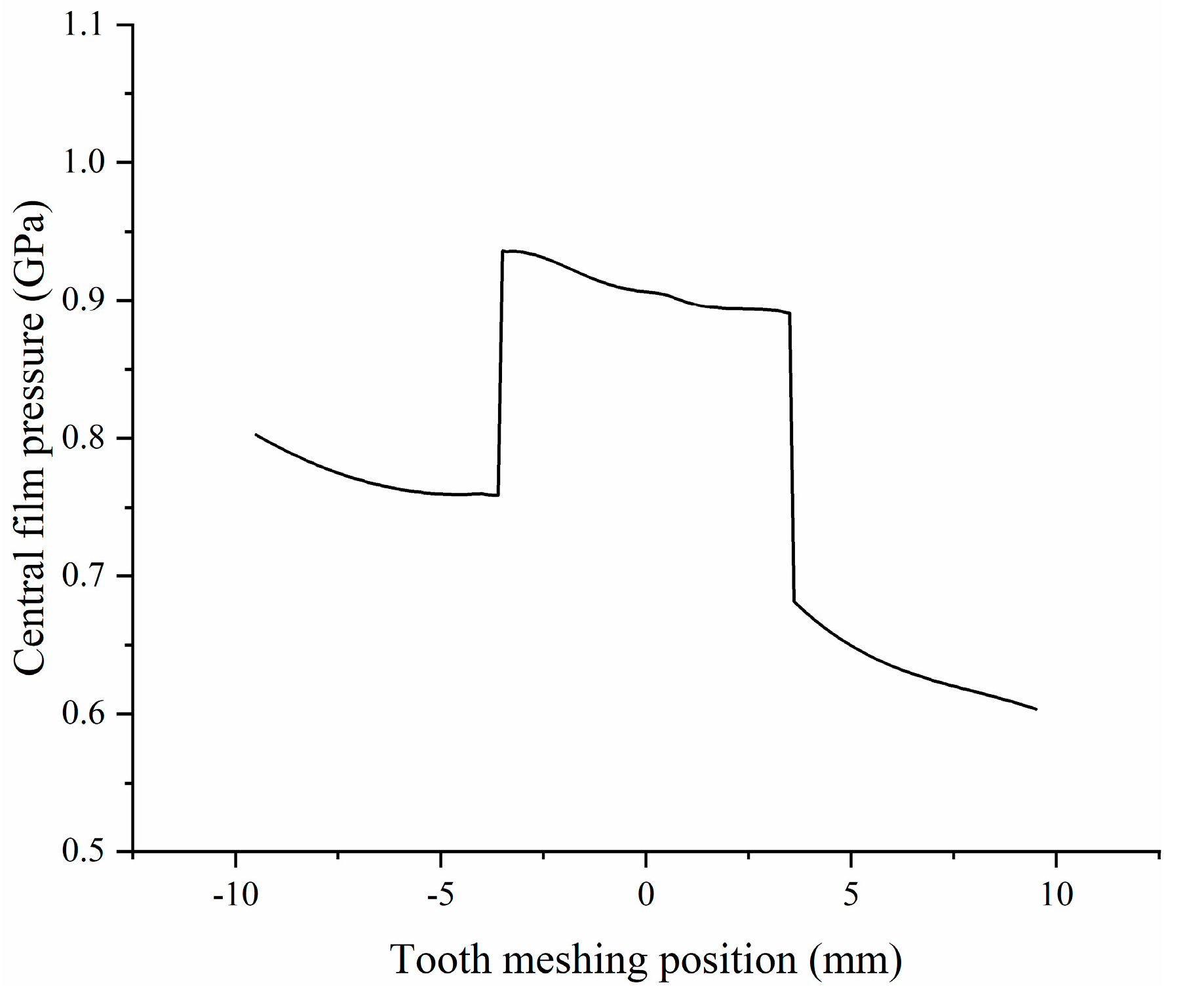
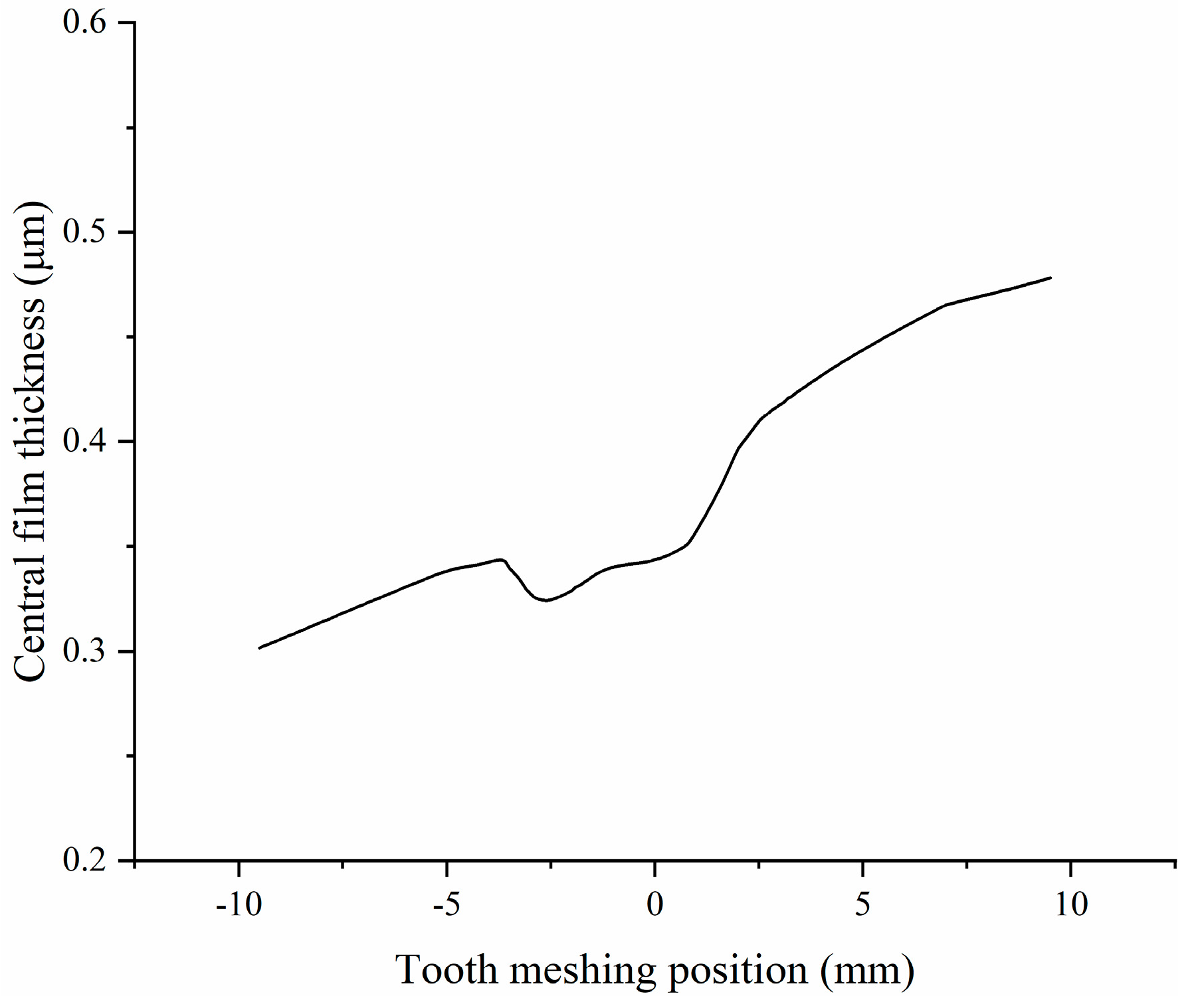
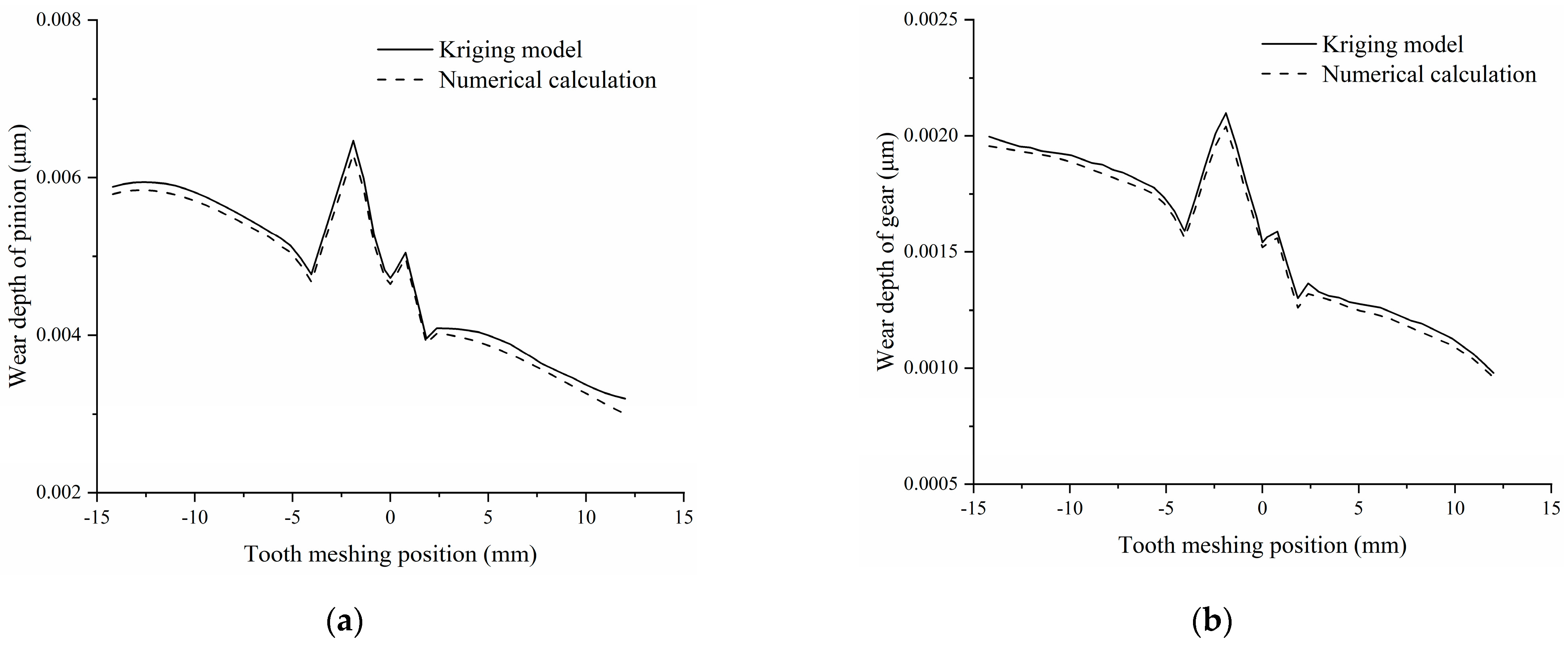
4. Results and Discussion

The parameters of gear dimensions and material properties required to calculate the wear of the gear are shown in

Table 1. Parameters required for calculation.

Parameters	Pinion	Gear
$\mathrm{Number}\mathrm{of}\mathrm{teeth}{n}_{1,2}$	16	24
Module m (mm)	4.5	4.5
$\mathrm{Pressure}\mathrm{angle}\alpha$ (deg)	$20°$	$20°$
Tooth width b (mm)	15	15
$\mathrm{Center}\mathrm{distance}{a}_w$ (mm)	91.5	91.5
Modification coefficient	0.8635	0.5
Modulus of elasticity E (Gpa)	210	210
$\mathrm{Poisson}\text{’}\mathrm{s}\mathrm{ratio}\nu$	0.3	0.3

. The lubricant is SAE 30.

The torque, speed, surface hardness, surface roughness and wear coefficient are important factors affecting gear wear. Therefore they are used as random variables, and each random variable obeys normal distribution. The mean and standard deviation of the random variables are shown in

Table 2. Distribution information of variables.

Variable	Distribution	Mean	Standard Deviation
Torque T (N m)	Normal	302	10
Speed v (rpm)	Normal	150	30
Hardness hd (GPa)	Normal	2.35	0.2
$\mathrm{Roughness}\sigma$$(\mathsf{\mu }\mathrm{m}$)	Normal	0.25	0.02
Wear coefficient K	Normal	$5\times {10}^{-4}$	$1\times {10}^{-4}$

.

The variation of the central film pressure along the line of action is shown in Figure 4. The central film pressure in the single tooth-meshing zone is greater than that in the double tooth-meshing zone. The central film pressure is also higher from the beginning of engagement because of the small roll suction speed and equivalent radius of curvature, although the load is smaller. The central film pressure in the single tooth-meshing zone decreases along the line of action, which is mainly caused by the change of the roll suction speed and equivalent radius of curvature.

The curve of the central film thickness along the line of action is shown in Figure 5. The film thickness is thinner at the beginning of engagement although the load is smaller due to the equivalent radius of curvature and the roll suction speed. The central film thickness has an increasing trend along the line of action, which is attributed to the increase in the roll suction speed. However, it has an abrupt drop in the middle part, which is due to a sudden change in load during the transition between the double- and single-tooth meshing of gears.

The gears’ wear depth after $1.5\times {10}^5$ revolutions of gear operation is shown in Figure 6. The pitch wear depth is the smallest, the root wear depth exceeds the top wear depth, and the pinion wear depth exceeds the gear wear depth. Compared with Ref. [8], the wear behavior of gears under mixed elastohydrodynamic lubrication is similar to that of dry friction. However, tooth wear under mixed lubrication is very much smaller than under dry friction for the same tooth profile parameters and operating parameters. This indicates that the rational use of lubricants can greatly reduce the reduction of tooth wear.

A Kriging model was developed using 100 samples. The variation curves of the maximum wear of gears are shown in Figure 7a,b. The accuracy of the model is an analysis of the progressive wear process of both the precise model and the proxy model where the random input values are deterministic and equal to the mean. As can be seen from Figure 7a,b, the wear depth increases cumulatively with time and the gear wear depth simulated by the Kriging model is very close to the actual wear depth. The accuracy of the Kriging model in approximating the actual wear depth is very high.

The goodness of fit refers to taking a certain number of samples outside the training samples to form a test set when the time is deterministic, and then the actual values of gear wear are compared with the predicted values of the Kriging model on the test set. Thirty sets of data were tested in the aforementioned Kriging model. The actual values of the samples were compared with the predicted values of the Kriging model, and the goodness of fit of the Kriging model was 0.9974. The actual wear depth and predicted wear depth of wear using the Kriging model are shown in Figure 8.

The wear depth from the Kriging model is compared to the results of another pair of gears derived from the numerical calculation to validate the correctness and generality of the Kriging model. The parameters are shown in

Table 3. Main parameters required for the Kriging model.

Parameters	Pinion	Gear
$\mathrm{Number}\mathrm{of}\mathrm{teeth}{n}_{1,2}$	32	96
Module m (mm)	5	5
$\mathrm{Pressure}\mathrm{angle}\alpha$ (deg)	$20°$	$20°$
Tooth width b (mm)	50	50
Contact load F (KN)	25	25
Speed v (rpm)	100	100
Hardness hd (GPa)	2.3	2.3
$\mathrm{Roughness}\sigma$$(\mathsf{\mu }\mathrm{m}$)	1	1
Wear coefficient K	$5\times {10}^{-4}$	$5\times {10}^{-4}$

.

It can be found that the results after $1\times {10}^5$ revolutions from the Kriging model correlate quite well with those from the calculation of the pinion wear depth for the mixed elastohydrodynamic lubrication, particularly near the pitch in Figure 9. In comparison to numerical calculation, it takes only a few minutes to obtain the wear depth of gears by the Kriging model, and the model’s accuracy in approximating real wear is quite high.

An important application of the Kriging model is to solve the reliability problem. In reliability studies, the time it takes to set up the original sample accounts for a large percentage of the total, usually about 99 percent or more. For the reliability problem of gear wear under mixed elastic flow lubrication, the Monte Carlo method is a widely accepted method, but it requires a large number of samples. If this method is used for reliability analysis of the implicit response function of gear wear, a large number of calculations are difficult to complete in a short time due to the low efficiency of a single calculation. Assuming that it takes 90 min to complete a gear wear calculation under mixed elastohydrodynamic lubrication and the study of gear wear reliability requires a sample space with an original sample size of $1\times {10}^5$, the number of numerical calculations and the time required for the Monte Carlo method and the Kriging model is shown in

Table 4. Consuming time of the MCS method and Kriging model.

Method	Number of Calculations	Time
Kriging MCS	100	150 h
Direct MCS	$1\times {10}^5$	17 years

. The time of the direct MCS method is unacceptable. It can be seen that the established Kriging model for gear wear with mixed elastohydrodynamic lubrication can accurately predict the approximate values of sample points, reduce the number of numerical calculations, and save a lot of time cost for the further study of gear wear.

5. Conclusions

In this paper, a model for computing gear wear under mixed elastohydrodynamic lubrication is constructed using the modified Reynolds equation, surface deformation model, elastoplastic micro-contact model, and modified Archard wear model. An approximate proxy model is created using the Kriging method to establish the direct relationship between gear parameters and wear, providing a novel way to predict gear wear. We have come to the following conclusions:

• Under mixed elastohydrodynamic lubrication, the tooth surface load is supplied by the oil film and the micro-convex of the tooth surface, and tooth surface wear occurs in the micro-convex contact;
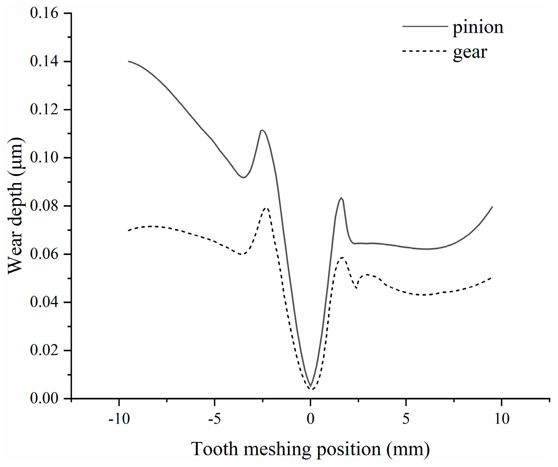
• The smallest wear occurs at the pitch, the wear at the root is more than the wear at the top, and the pinion wear is greater than the gear wear;
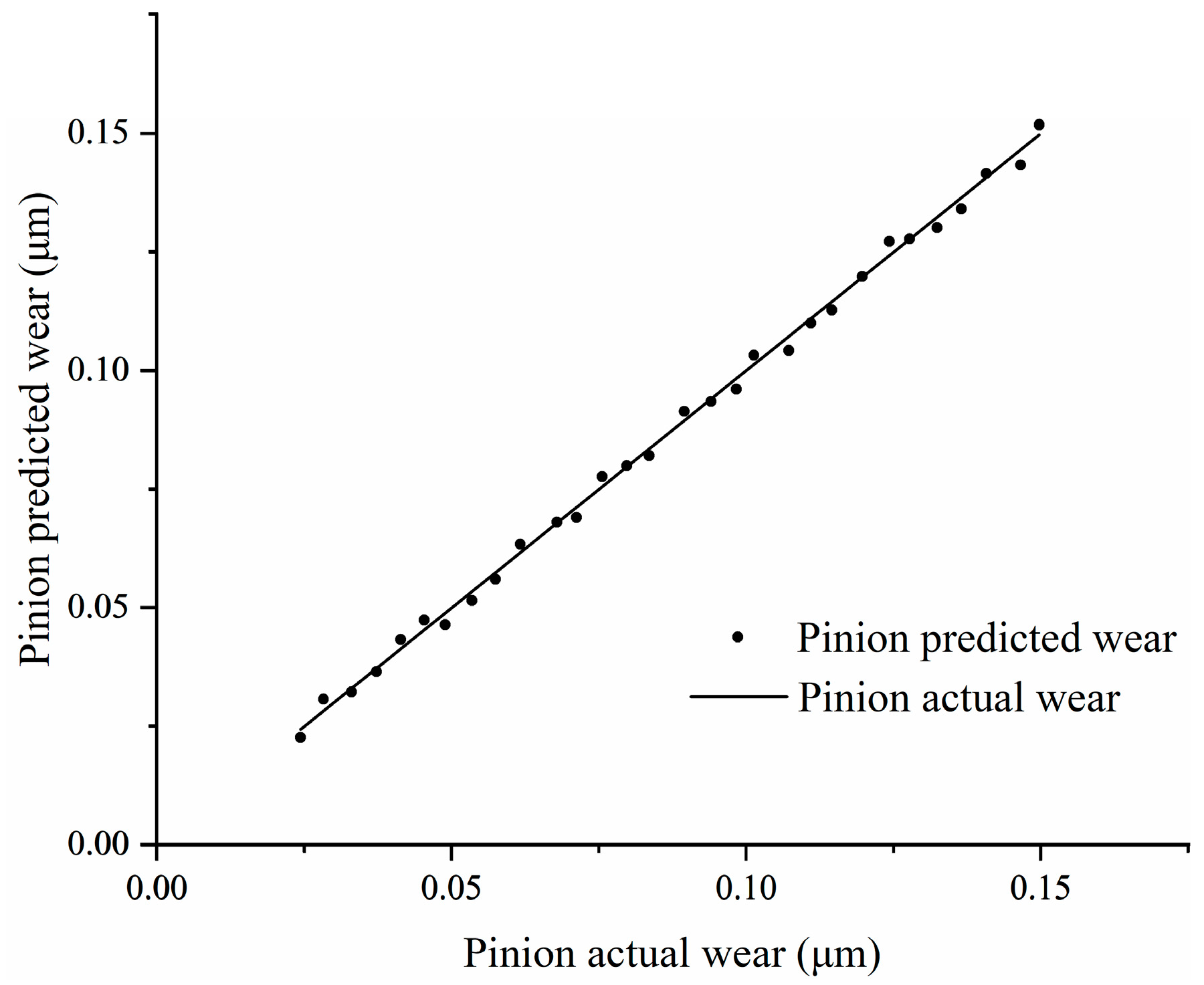
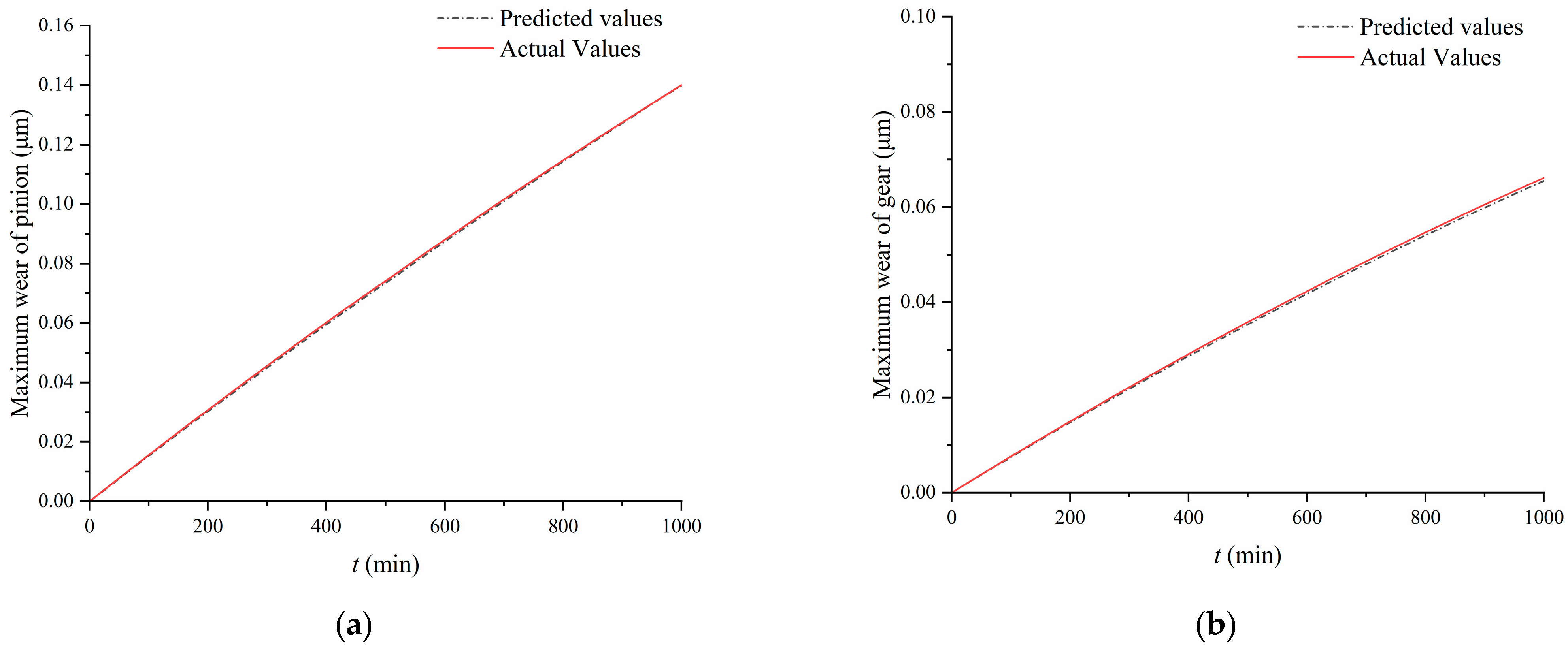
• The Kriging model may replace the numerical wear model with a limited number of samples, and the fit is excellent. This gear wear model may be used to increase the accuracy and efficiency of calculations in mixed elastohydrodynamic lubrication and to forecast unknown wear.

References

1. Ding, H. Dynamic Wear Models for Gear Systems. Ph.D. Thesis, The Ohio State University, Columbus, OH, USA, 2007. [Google Scholar]
2. Atanasiu, V.; Oprisan, C.; Leohchi, D. The effect of tooth wear on the dynamic transmission error of helical gears with smaller number of pinion teeth. Appl. Mech. Mater. 2014, 657, 649–653. [Google Scholar] [CrossRef]
3. Kuang, J.H.; Lin, A.D. The effect of tooth wear on the vibration spectrum of a spur gear pair. J. Vib. Acoust. 2001, 123, 311–317. [Google Scholar] [CrossRef]
4. Choy, F.K.; Polyshchuk, V.; Zakrajsek, J.J.; Handschuh, R.F.; Townsend, D.P. Analysis of the effects of surface pitting and wear on the vibration of a gear transmission system. Tribol. Int. 1996, 29, 77–83. [Google Scholar] [CrossRef]
5. Mackaldener, M.; Flodin, A.; Andersson, S. GDN-5 Robust noise characteristics of gears due to their application, manufacturing errors and wear(Gear dynamics and noise). In Proceedings of the JSME International Conference on Motion and Power Transmissions I(01-202), Fukuoka, Japan, 15 November 2001; pp. 21–26. [Google Scholar]
6. Chen, Y.; Matubara, M. GSD-2 Effect of automatic transmission fluid on pitting fatigue strength of carburized gears (Gear Strength and durability). In Proceedings of the JSME International Conference on Motion and Power Transmissions I(01-202), Fukuoka, Japan, 15 November 2001; pp. 151–155. [Google Scholar]
7. Archard, J.F. Contact and Rubbing of Flat Surfaces. J. Appl. Phys. 1953, 24, 981–988. [Google Scholar] [CrossRef]
8. Flodin, A.; Anderson, S. Simulation of mild wear in spur gears. Wear 1997, 207, 16–23. [Google Scholar] [CrossRef]
9. Lundvall, O. Simulation of Contact, Friction, and Wear in Gears-a Finite Element Approach. Ph.D. Thesis, Linköping University, Linköping, Sweden, 2000. [Google Scholar]
10. Lundvall, O.; Klarbring, A. Simulation of wear by use of a nonsmooth newton method-a spur gear application. Wear 2003, 254, 1216–1232. [Google Scholar]
11. Park, D.; Kolivand, M.; Kahraman, A. Prediction of surface wear of hypoid gears using a semi-analytical contact model. Mech. Mach. Theory 2012, 52, 180–194. [Google Scholar] [CrossRef]
12. Park, D.; Kolivand, M.; Kahraman, A. An approximate method to predict surface wear of hypoid gears using surface interpolation. Mech. Mach. Theory 2014, 71, 64–78. [Google Scholar] [CrossRef]
13. Johnson, K.L.; Greenwood, J.A.; Poon, S.Y. A simple theory of asperity contact in elastohydro-dynamic lubrication. Wear 1972, 19, 91–108. [Google Scholar] [CrossRef]
14. Sander, D.E.; Allmaier, H.; Priebsch, H.H.; Witt, M.; Skiadas, A. Simulation of journal bearing friction in severe mixed lubrication—Validation and effect of surface smoothing due to running-in. Tribol. Int. 2016, 96, 173–183. [Google Scholar] [CrossRef] [Green Version]
15. Sharma, S.C.; Phalle, V.M.; Jain, S.C. Influence of wear on the performance of a multirecess conical hybrid journal bearing compensated with orifice restrictor. Tribol. Int. 2011, 44, 1754–1764. [Google Scholar] [CrossRef]
16. Zhang, Y.; Cao, H.; Kovalev, A.; Meng, Y. Numerical running-in method for modifying cylindrical roller profile under mixed lubrication of finite line contacts. J. Tribol. 2019, 141, 041401. [Google Scholar] [CrossRef]
17. Winkler, A.; Marian, M.; Tremmel, S.; Wartzack, S. Numerical Modeling of Wear in a Thrust Roller Bearing under Mixed Elastohydrodynamic Lubrication. Lubricants 2020, 8, 58. [Google Scholar] [CrossRef]
18. Zhu, G. Valve Trains—Design Studies, Wider Aspects and Future Developments. Eng. Tribol. 1993, 26, 183–211. [Google Scholar]
19. Wu, S.; Cheng, H.S. Sliding wear calculation in spur gears. J. Tribol. 1993, 115, 493–500. [Google Scholar] [CrossRef]
20. Patir, N.; Cheng, H.S. An average flow model for determining effects of three-dimensional roughness on partial hydrodynamic lubrication. J. Lubr. Technol. 1978, 100, 12–17. [Google Scholar] [CrossRef]
21. Patir, N.; Cheng, H.S. Application of average flow model to lubrication between rough sliding surfaces. J. Tribol. 1979, 101, 220–230. [Google Scholar] [CrossRef]
22. Dowson, D. A generalized Reynolds equation for fluid-film lubrication. Int. J. Mech. Sci. 1962, 4, 159–170. [Google Scholar] [CrossRef]
23. Majumdar, B.C.; Hamrock, B.J. Effect of surface roughness on elastohydrodynamic line contact. J. Lubr. Technol. 1982, 104, 401–409. [Google Scholar] [CrossRef]
24. Greenwood, J.A.; Tripp, J.H. The contact of two nominally flat rough surfaces. P I Mech. Eng. 1970, 185, 625–663. [Google Scholar] [CrossRef]
25. Zhao, Y.; Maietta, D.M.; Chang, L. An Asperity microcontact model incorporating the transition from elastic deformation to fully plastic flow. J. Tribol. 2000, 122, 86–93. [Google Scholar] [CrossRef]
26. Masjedi, M.; Khonsari, M.M. Film thickness and asperity load formulas for line-contact elastohydrodynamic lubrication with provision for surface roughness. J. Tribol. 2012, 134, 011503. [Google Scholar] [CrossRef]
27. Masjedi, M.; Khonsari, M.M. An engineering approach for rapid evaluation of traction coefficient and wear in mixed EHL. Tribol. Int. 2015, 92, 184–190. [Google Scholar] [CrossRef]
28. Masjedi, M.; Khonsari, M.M. On the prediction of steady-state wear rate in spur gears. Wear 2015, 342–343, 234–243. [Google Scholar] [CrossRef]
29. Cheng, J.; Li, Q.S. Application of the response surface methods to solve inverse reliability problems with implicit response functions. Comput. Mech. 2009, 43, 451–459. [Google Scholar] [CrossRef]
30. Papadrakakis, M.; Lagaros, N.D. Reliability-based structural optimization using neural networks and Monte Carlo simulation. Comput. Method Appl. M 2002, 191, 3491–3507. [Google Scholar] [CrossRef]
31. Zhu, Z.F.; Du, X.P. Reliability analysis with Monte Carlo simulation and dependent kriging predictions. J. Mech. Des. 2016, 138, 121403. [Google Scholar] [CrossRef]
32. Laurenceau, J.; Sagaut, P. Building efficient response surfaces of aerodynamic functions with kriging and cokriging. AIAA J. 2008, 46, 498–507. [Google Scholar] [CrossRef] [Green Version]
33. Feng, J.L.; Sun, Z.L.; Zhao, J.; Zhang, J.; Liang, C.F. Vibration reliability analysis on a spindle system based on AK-MCS method. Chin. J. Vib. Shock 2019, 38, 135–140. [Google Scholar]
34. Yang, L.; Tong, C.; Chen, C.; Guo, Q.P. Vibration reduction optimization of gear modification based on Kriging model and genetic algorithm. Chin. J. Aerosp. Power 2017, 32, 1412–1418. [Google Scholar]
35. Tian, X. Maximum and Average Flash Temperatures in Sliding Contacts. J. Tribol. 1994, 116, 167–174. [Google Scholar] [CrossRef]
36. Matheron, G. The intrinsic random functions and their applications. Adv. Appl. Probab. 1973, 5, 439–468. [Google Scholar] [CrossRef] [Green Version]
Figure 1. Gear meshing relationship.
Machines 10 00490 g001
Figure 2. Flowchart of the calculation of the gear wear under mixed elastohydrodynamic lubrication.
Machines 10 00490 g002
Figure 3. Flowchart for building the Kriging model.
Machines 10 00490 g003
Figure 4. The variation of the central film pressure.
Machines 10 00490 g004
Figure 5. The curve of the central film thickness.
Machines 10 00490 g005
Figure 6. Wear depth of the pinion and gear.
Machines 10 00490 g006
Figure 7. Calculation accuracy of the Kriging model: (a) Pinion; (b) Gear.
Machines 10 00490 g007
Figure 8. Actual wear depth and prediction based on Kriging model.
Machines 10 00490 g008
Figure 9. Wear depth of the Kriging model compared to the results of the numerical calculation: (a) Pinion; (b) Gear.
Machines 10 00490 g009