Abstract
While the size of the four-bar linkage is the basis of kinematic performance analysis in a beam pumping unit, there is still a lack of effective and direct measurement of it. Since the motor input power and the polished rod position are commonly used production data, a size identification algorithm of the four-bar linkage based on the motor input power and the polished rod position is proposed in this paper. Firstly, the kinematic model of a beam pumping unit, the speed model of a motor, the initial value, and the state space model are established. Secondly, a Cubature Kalman filter with nonlinear constraints is designed and the size identification algorithm is worked out. Lastly, the model and the size identification algorithm are validated based on the simulated and measured data, and the characteristics of identification with different measurement covariance are studied. The results demonstrate that both the model and the algorithm are feasible. The maximum relative error between the identified and the real size increases from 0.23% to 9.37% when the covariance increases from 10−6 to 10−1. With the measured covariance of the polished rod velocity, the maximum relative error is 7.09%. A comparison of several current identification methods demonstrates that the proposed algorithm is more accurate.
1. Introduction
As a major production equipment in the oilfield, the beam pumping unit enjoys huge installed capacity worldwide [1]. It possesses the advantages of simplicity, reliability, ease of operation and maintenance, and adaptability to harsh environments [2,3].
A sucker-rod pumping system is composed of the downhole pump, the sucker-rod string, the surface pumping unit, the gear reducer (gearbox), the V-belt drive, and the prime mover [4]. As a typical sucker-rod pumping system, the beam pumping unit has a distinctive surface pumping unit of a four-bar linkage, with the cranks, the linkage rod, walking beam, the standard bar, and the horsehead [5,6,7].
The four-bar linkage can convert the motor’s rotary motion, which is decelerated by the belt and gearbox drive into the oscillatory motion of the polished rod. It is one of the key mechanisms of the beam pumping unit. The size of the four-bar linkage is crucial to the contour size and the working performance of the beam pumping unit [8]. Only when its size is known can the position, velocity, and acceleration of the polished rod and the torque factors as functions of crank angle be calculated [7]. In addition, the crank radius also determines the balance of the beam pumping unit, which is closely related to the energy consumption or even the service life of the beam pumping unit [9]. Therefore, the size of the four-bar linkage is of vital importance for the design, behavior prediction, and state detection of a beam pumping unit. In recent years, some new technologies, such as the indirect measurement DC based on measured motor power [10], fault diagnosis based on motor power curves [11,12], prediction of submergence depth based on a hybrid model [5], and variable speed drive technology of beam pumping units [13], require a more accurate size for the four-bar linkage.
However, it is difficult to measure the sizes of the four-bar linkage directly in actual production because of their large size and the continuous motion of the four-bar linkage. Sun et al. [14] proposed a kinematic analysis model of a beam pumping unit based on deep learning, which can give the size of the four-bar linkage. The method is built on the real-time video stream taken by the mobile robot, which is easily affected by the camera and the weather. At present, most of the size of the four-bar linkage is supplied by manufacturers. Obviously, it cannot reflect the actual size, because the size will change due to the equipment installation or a long-time operation. Since the polished rod position and the motor input power are the primary real-time data monitored continuously [10], it is necessary to measure the sizes of the four-bar linkage with a soft method. In this paper, an identification method will be proposed based on the measured polished rod position and the motor input power.
Parameter identification plays an important role in controller design, dynamic systems modeling, and signal processing [15,16,17]. More mainstream identification methods have been proposed for linear systems and nonlinear systems, such as the recursive least squares (RLS) methods [18,19], the stochastic gradient descent (SGD) methods [20,21], the artificial neural network (ANN) techniques [22,23], and the Kalman filter. For linear time invariant systems, the RLS method is widely used and easy implemented [24,25] but susceptible to noise [26]. The SGD method involves a small amount of calculation with a low accuracy [27]. The ANN technique benefits from higher accuracy as well as convenience in modeling but demands a training process [28].
Notably, the Kalman filter (KF) is typical, effective, and still widely used with the merits of real time, fast speed, and strong anti-interference ability [29]. The Kalman filter was proposed by Kalman in 1960 [30], and is only suitable for linear systems. With a view to apply the Kalman filter to nonlinear spacecraft navigation, the extended Kalman filter (EKF) was originally proposed by Stanley Schmidth in 1967 [31,32]. The basic idea of EKF is utilizing the value of first-order nonlinear Taylor expansion around the estimated status [33]. However, the EKF can lead to unstable results when the nonlinearity in the system is strong [34]. To overcome this theoretical deficiency, the unscented Kalman filter (UKF) was first proposed by Julier et al. in 1995 [35], with unscented transformation (UT) as its core [36]. Considering the deterioration and even divergence of the filter performance when the state dimension of the system is more than 3 in UKF, Arasaratnam and Haykin [37] proposed a Cubature Kalman filter (CKF) algorithm based on cubature transform, which is an unconstrained state Cubature Kalman filter. In practical applications, physical limitations always impose some constraints on the states or parameters of the system [38], so it is of great significance to study the constrained Cubature Kalman filter (CCKF). Simon [39] summarized the various ways to incorporate state constraints into the Kalman filter and its nonlinear modifications, such as model reduction, estimate projection, probability density function, etc., which provides a guideline to research the constrained Kalman filter. Zarei and Shokri [38] proposed a CCKF algorithm, which integrates linear constraints into the CKF by projecting unconstrained CKF estimation onto the boundary of the admissible region. However, it needed a Taylor series expansion of the constraint equation.
A brief comparison of different identification methods is tabulated in Table 1.

Table 1.
Major pros and cons of identification methods.
From the above survey, there is still a lack of an effective method to measure the four-bar linkage sizes of the beam pumping units while the identification method will be a feasible scheme. Due to the strong non-linearity of the four-bar linkage mechanism motion, the CKF is the best choice. With the consideration of the limitations in the sizes identification of four-bar linkage, a nonlinear constrained Cubature Kalman filter (NCCKF) without Taylor series expansion should be further studied. In this paper, a NCCKF is employed to identify the sizes of the four-bar linkage.
The contributions of this paper are as follows:
- (1)
- A speed model of a motor is established. Based on the nameplate parameters and the input power, the motor speed can be obtained.
- (2)
- An initial value model is established. Based on the measured polished rod position, the initial value and the lower boundary and up boundary can be determined.
- (3)
- A NCCKF algorithm is proposed. Based on the maximized conditional probability density function, the predicted state is modified by solving the constrained optimization problem.
- (4)
- A size identification algorithm based on the measured motor input power and the polished rod position is proposed.
2. System Model
2.1. Kinematic Model of A Pumping Unit
The geometric diagram of the four-bar linkage in a beam pumping unit is shown in Figure 1, where R is the radius of the crank, P is the length of the pitman, C is the length of the rear arm of walking beam, A is the length of the forearm of walking beam, and K is the length of the fixed bar.
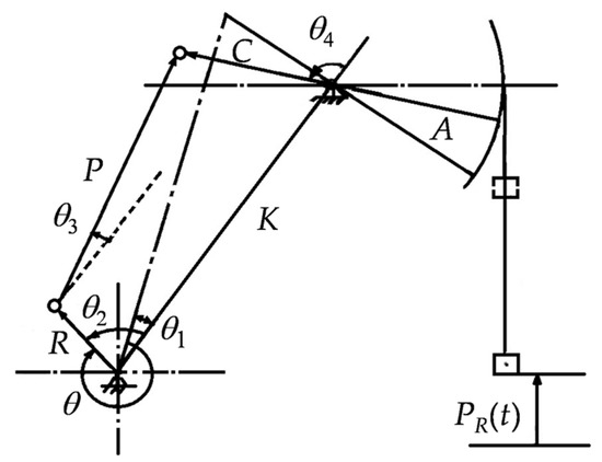
Figure 1.
Geometric diagram of the four-bar linkage in a beam pumping unit.
As is illustrated in Figure 1, when the crank rotates clockwise and the polished rod starts from the bottom of the stroke, it has
When the sizes of R, C, P, and K are known, the angles of θ3(t) and θ4(t) can be solved according to the following equation:
Thus, the polished rod position is obtained by
The polished rod velocity and acceleration are given by
where [7]
Therefore, the established kinematic model of a pumping unit is as follows:
If the crank rotates anticlockwise, it has
Thus, if the kinematic data of the crank, i.e., angle, angular velocity, and angular acceleration, are known, the sizes of R, C, P, K, and A can be identified according to the measured polished rod kinematic data–that is, the polished rod position, velocity, and acceleration. In actual production, the measured data are the polished rod position, and the polished rod velocity and acceleration can be obtained by differentiating them.
2.2. Speed Model of A Motor
Most of the prime movers of the beam pumping units are three-phase asynchronous motors (referred to as motor for convenience). When the belt drive does not slip, the crank angle will be proportional to the motor output shaft angle. Thus, if the motor speed can be determined, the crank angle, velocity, and acceleration can be calculated. Since it is easy to obtain the input power of a motor in real-time [10], it is necessary to establish a motor speed model based on the input power.
As is shown in Figure 2 [40,41], most of the equivalent circuit of a motor is T-circuit. When the values of the circuit parameters R1, R2, X1, X2, and Xm, are given, the motor torque and the input power can be calculated as follows without consideration of the mechanical loss:
where
and ns is the synchronous speed of the motor.
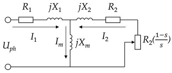
Figure 2.
T-type reduced to one-phase equivalent circuit of a motor.
As is shown in Equations (10) and (11), and Figure 2, the motor torque and the input power are rather complicated with the T-circuit because of its two serial–parallel branches. Thevenin approach can be used to establish the speed model and it is shown in Figure 3.
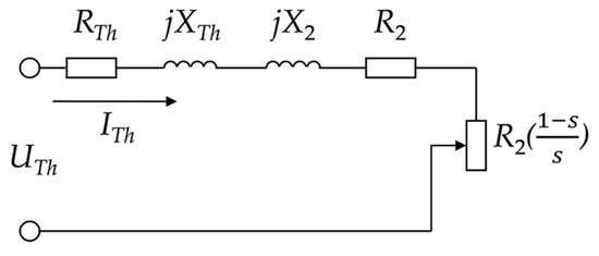
Figure 3.
Thevenin’s one-phase equivalent circuit for a motor.
Circuit parameters UTh, RTh, and XTh are determined with the Kirchhoff circuit rules as follows [40]:
According to Figure 3, the rotor current is given by
Thus, the power dissipated across the stator resistance RTh is given by
The total power transferred across the air gap from the stator is given by
Without consideration of the mechanical loss, the total input power is given by
According to Equation (15), Equations (16) and (17) can be rewritten as:
Thus, it has the maximum power PMm and the maximum slide Sm in the motor state [42] according to Equation (20):
According to Equation (21), Equations (19) and (20) can be written as:
where
Thus, the total input power is given by
Resolving Equation (25) yields the slide
where
Therefore, it has the motor speed:
Thus, the motor speed can be calculated based on the input power when the parameters of PMm, Sm, and σ are given. There are two methods to determine these parameters. One is to calculate it based on Equations (21) and (24) according to the circuit parameters, the other is according to the nameplate parameters. The nameplate parameters include the rated power PH, rated slide SH, rated efficiency ηH, and maximum torque ratio λk. It has
To determine σ, the rated efficiency ηH should be used. In view of the output motor power, it has:
For , it has the normal efficiency according to Equations (25) and (30)
Therefore, it has:
Since the crank angle is proportional to the motor output shaft angle, it has the angular velocity as follows:
where iMB is a transmission ratio and np is the pumping speed.
Thus, the crank angle can be obtained by integrating the angular velocity, and the acceleration can be obtained by differentiating the angular velocity.
2.3. Initial Value and State Space Model
The initial value of the parameter is very important for the parameter identification.
According to the movement of the crank slider mechanism, the polished rod position can be approximated as follows [43]:
where
The values of the λ1 and λ2 can be determined according to the optimization problems:
where θ(Na) = 0.8θm, θm is the crank angle of the maximum polished rod position.
In the design of the beam pumping unit, the maximum crank radius Rm0, the length of the pitman, and the rear arm of the walking beam have the relative size restrictions, that is [44]:
If the intermediate value in Equation (37) is taken, it has an initial value of R/C according to Equation (35), that is, R/C = 1.4λ2.
Thus, the initial value of the identification can be calculated according to the symmetrical cycle working mode of a beam pumping unit [44].
where PRm is the maximum value of the polished rod position.
In the design of the beam pumping unit, the relative size restrictions among each rod length of the four-bar linkage are as follows [45]:
According to the resolution of optimization problems of Equation (36) and the restriction of Equation (39), its restriction is as follows:
To avoid complex numbers in angle calculations, it has the nonlinear constraint:
In this paper, the identified parameter is the size of the four-bar linkage, and the measured data are the polished rod position, velocity, and acceleration. Therefore, it has the state and measured vector of
The state equation and the measurement equation are as follows:
where
where w(t) and v(t) are the independent process and the observation Gaussian nose with zeros means and covariances Qc and Rc, respectively. I5 is 5-dimensional identity matrix.
According to Equation (38), the initial value is
And the nonlinear constraint is
where
After the state equation is discretized, it has:
3. Design of Cubature Kalman Filter with Nonlinear Constraints
This section aims to find a Cubature Kalman filter algorithm with nonlinear constraint to identify the size of the four-bar linkage.
3.1. Cubature Kalman Filter without Constraint
The identification in this paper is a nonlinear problem and it has five state variables. Therefore, the Cubature Kalman filter is selected.
The Cubature Kalman filter is a Bayesian filter theory in the Gaussian domain and a set of volume points is employed to approximate the state mean and covariance of non-linear systems based on the third-order spherical radial cubature criterion [37].
The CKF algorithm is summarized below [37,38]:
Step 1. Initialize with
Step 2. Decompose covariance by Cholesky
Step 3. Evaluate the cubature points, i = 1, 2,..., m (where m = 2n):
where is the i-th element of the following set [46]:
, and is n-dimensional identity matrix.
Step 4. Evaluate the propagated cubature points, i = 1, 2,..., m (where m = 2n):
Step 5. Estimate the predicted state and predicted error covariance:
Step 6. Decompose covariance by Cholesky:
Step 7. Redraw cubature points:
Step 8. Estimate the predicted measurement and associated covariance:
Step 9. Estimate the cubature Kalman gain:
Step 10. Update the state estimation and associated covariance:
Step 11. Go to step 2 for the next sample.
3.2. Cubature Kalman Filter with Nonlinear Constraint
The essence of the Kalman filter is that its estimate is that value of that maximizes the conditional probability density function [47]:
Therefore, if the Kalman filter is constrained, an estimate should be found to maximize the conditional probability with satisfying the constraint [47], so it has the constrained optimization problems in this paper:
Notably, when is replaced by any symmetric positive definite weighting matrix W, the maximum probability method is the projection method. With consideration of the characteristics of cubature transform, the projection method of cubature points in the Cubature Kalman filter [37] can be modified, and the checking and modifying between step 6 and step 7 of the ordinary CKF algorithm should be added. It is
NCCKF step 1. Check the state estimation
if is out of constraint,
resolve constrained optimization problem:
And update the state, that is .
Otherwise, turn to the step 7 of the ordinary CKF algorithm.
The optimization problem of Equation (51) can be easily resolved by the active-set method.
The size identification algorithm is summarized in Algorithm 1.
| Algorithm 1. Size identification of a four-bar linkage. |
| Input series: PR(t), vR(t), aR(t), Pin(t), input parameters: np, iMB, PH, SH, ηH, λk, Qc, Rc. |
| 1. Calculate (t) according to (28) and (33), then calculate θ(t) and (t) 2. Obtain θm, calculate λ1 and λ2 according to (36) and then obtain x0, xL, and xH 3. Initialize w, v, P00, 4. for k = 2:N 5. Decompose covariance 6. Evaluate the cubature points and obtain 7. Evaluate the propagated cubature points and obtain 8. Estimate the predicted state and predicted error covariance, then obtain , 9. Decompose covariance and obtain 10. Check the state estimation if is out of constraint Resolve constrained optimization problem (51) and update the state end 11. Redraw cubature points and obtain 12. Estimate the predicted measurement and associated covariance, then obtain ,,, 13. Estimate the cubature Kalman gain and obtain 14. Update the state estimation and associated covariance, then obtain , 15. End 16. Output and plot ,, |
4. Validation and Analysis
In this section, the size identification algorithm will be validated based on the simulated and measured data. The first is the validation of the speed model based on the input power simulated by the T-type circuit motor model; the nameplate parameters and circuit parameters are given. The second is the validation of the size identification algorithm based on simulated the polished rod position, velocity, and acceleration. The third is the validation of the NCCKF algorithm based on the simulated polished rod position, velocity, and acceleration. The last is the validation of the size identification and result analysis based on the measured motor input power and the polished rod position of a beam pumping unit. MATLAB R2021a code is applied in this paper.
4.1. Validation of Speed Model
The nameplate parameters of the motor are shown in Table 2 and its T-type equivalent circuit parameters are R1 = 0.3958 Ω, X1 = 0.4002 Ω, R2 = 0.8837 Ω, X2 = 2.1085 Ω, and Xm = 13.0658 Ω, respectively. Thus, the parameters of the Thevenin equivalent circuit can be calculated according to Equation (14).

Table 2.
Nameplate parameters of the motor.
In view of the fluctuating load of the beam pumping unit, the output torque of the motor is set as:
The pumping speed of the beam pumping unit is 1.7 times/min.
According to Equations (10) and (11), the input power of the T-type equivalent circuit motor model can be calculated and shown in Figure 4. Thus, the speed can be calculated based on the circuit parameters and Equations (21), (24) and (28). For comparison purposes, the above speed is defined as circuit speed. The other speed can be calculated according to Equations (28), (29) and (32) based on the nameplate parameters, which are defined as the nameplate speed for comparison purposes. The results are all shown in Figure 4. As is illustrated in Figure 4, the nameplate speed is consistent with the circuit speed and the relative error is 0.12%, which indicates that the speed model is effective. Here, the relative error represents the ratio of the maximum error between the nameplate speed and the circuit speed to the maximum value of the circuit speed.
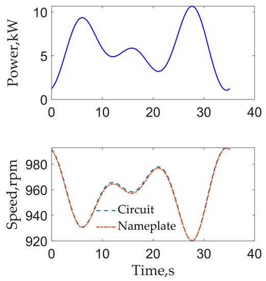
Figure 4.
Simulated input power and speed curve.
4.2. Validation of Size Identification Algorithm Based on the Simulated Data
The type of the beam pumping unit is CYJY10-4.2-53HB. The real values of the size are shown in Table 3.

Table 3.
Real and identified size identification.
The crank velocity can be calculated according to the nameplate motor speed shown in Figure 4 when iMB is 0.01 according to Equation (33). Thus, the crank angle and acceleration can be obtained by integrating and differentiating the crank velocity. They are all shown in Figure 5.
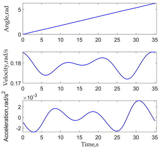
Figure 5.
Calculated crank angle, velocity, and acceleration.
Based on the crank angle, velocity, and acceleration, the polished rod position PR(t), velocity vR(t) and acceleration aR(t) can be simulated according to Equation (8) with the real values of the size listed in Table 3. The simulated results are shown in Figure 6. The Equation (3) can be solved by the fsolve function of MATLAB. Now, it has the measurement series for the size identification, that is PR(t), vR(t), and aR(t).
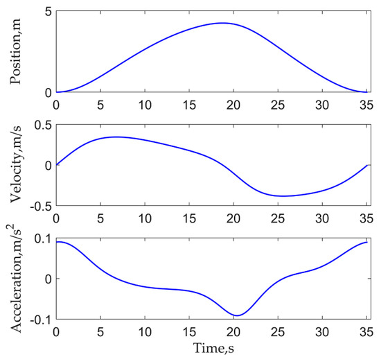
Figure 6.
Simulated polished rod position, velocity, and acceleration.
According to the polished rod position shown in Figure 6, it has the maximum value at position of 3.3796 rad and the series length N is 118. The solution of Equation (36) with the fminunc function of MATLAB obtains the value of λ1 and λ2. The simulated polished rod position, the redrawn position based on Equation (34) with the real values, and that based on Equation (34) with the solved values of λ1 and λ2 are shown in Figure 7. As is illustrated in Figure 7, the real value position is consistent with the solved value position and the relative error is 1.12%, which shows that the method to obtain the values of λ1 and λ2 by solving Equation (36) is feasible.
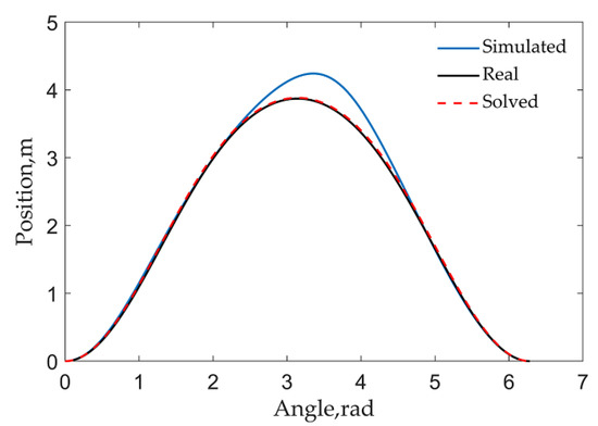
Figure 7.
Simulated, real, and solved polished rod position.
So, the initial value, lower boundary, and up boundary can be calculated according to Equations (38) and (40) as follows
When Qc = 10−7I5, Rc = 10−3I5 and P00 = 0.15I5, the size of the four-bar linkage can be identified according to the Algorithm 1. Checking the calculation process shows that the algorithm can run without constraints under this initial value. So, the algorithm is based on the ordinary CKF algorithm. The outputs of and , that is the simulated and predicted measurement data, are plotted in Figure 8, which shows that simulated and predicted polished rod position and velocity have good consistency. Predicted polished rod acceleration has a disturbance at the beginning, but it is updated to the simulation acceleration soon. The output of , that is identified size results of four-bar linkage, is plotted in Figure 9. For comparison, the real size values are also plotted in Figure 9. Figure 9 shows that the identified sizes can be from their initial values to the corresponding real values within the first 10 s. The last values of are shown in Table 3. For comparison, the relative error between the identified and real values is also shown in Table 3. As listed in Table 3, the relative error of K is the maximum of 4.94% and the relative error of A is the minimum with 0.48%. Interestingly, the relative errors of R, C, P, and K are basically equal. The reason is that the polished rod position is only sensitive to the ratios between the sizes shown in Equations (3) and (4). The above results show that the algorithm proposed in this paper is feasible.
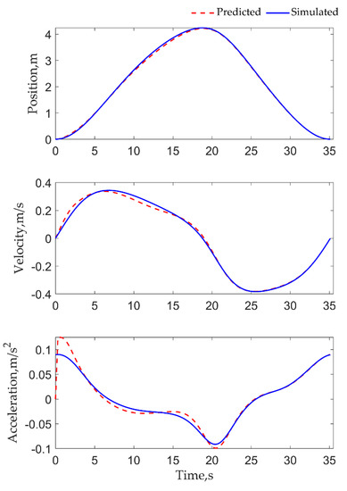
Figure 8.
Simulated and predicted measurement data.
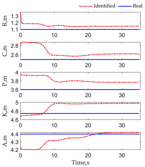
Figure 9.
Identified size results.
To illustrate the affection of the measurement covariance Rc, the size of the four-bar linkage is identified according to the Algorithm 1 when Rc increases from 10−6 to 10−1, that is, Rc1 = 10−6, Rc2 = 10−5, Rc3 = 10−4, Rc4 = 10−3, Rc5 = 10−2, and Rc6 = 10−1.
The relative error between the identified and the real values is shown in Table 4. As is listed in Table 4, with the increase in measurement covariance Rc, the relative error rises, which indicates that the accuracy of identification is reduced. Under the same covariance, the relative error of A is the minimum while that of R, C, P, and K is almost the same when the covariance is less than 10−1.

Table 4.
Relative error with different measurement covariances.
4.3. Validation of NCCKF Algorithm
If the initial value is inappropriate, the algorithm cannot run due to the arccosine operation in the model, and therefore the NCCKF algorithm is necessary. For the sake of validation of the NCCFK algorithm, K0 = 2P0, Qc = 10−7I5, and P00 = 0.15I5. Obviously, the ordinary CKF algorithm cannot run because the initial value is out of the constrained–that is, g(1) > 0 and g(2) > 0. The constrained optimization problem (51) is solved by fmincon function of MATLAB. When the covariances Rc increases from 10−6 to 10−1, the identified size is shown in Table 5.

Table 5.
Relative error with different measurement covariances.
As is shown in Table 5, the result follows the same rule as the ordinary CKF with the increase in covariances while the relative error of R, C, P, and K is almost 40%, which indicates that the algorithm is feasible but only converges to a local optimum value instead of the real value. If the ratio of A and C (or anyone among R, P, and K) is given, the size could be calculated because the value of A has been identified. On the other hand, these results also show the initial value model proposed in this paper is of vital importance for the size identification.
4.4. Validation of Size Identification Algorithm Based on the Measured Data
The measured field data are the series data of the polished rod position and motor in-put power in an oil well of Shengli Oilfield of PetroChina. The type of the beam pumping unit is CYJY10-3-53HB with the pumping speed of 2 times/min. The length N of the series is 121. The measured field data are presented in Figure 10. The velocity and acceleration obtained by differentiating the polished rod position are shown in Figure 11. As can be seen from Figure 11, the noises in the velocity and acceleration are loud. For direct illustration of the measurement noise, the polished rod position can be approximated by the truncated Fourier series [48] when the number of Fourier coefficients is 10. The corresponding approximated polished rod position, velocity, and acceleration are also shown in Figure 11.
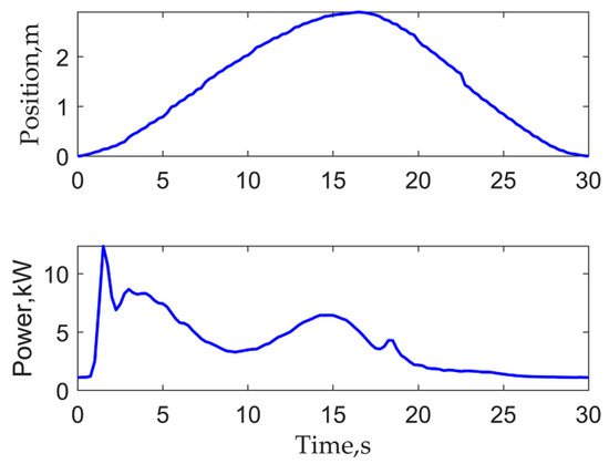
Figure 10.
Measured oilfield data.
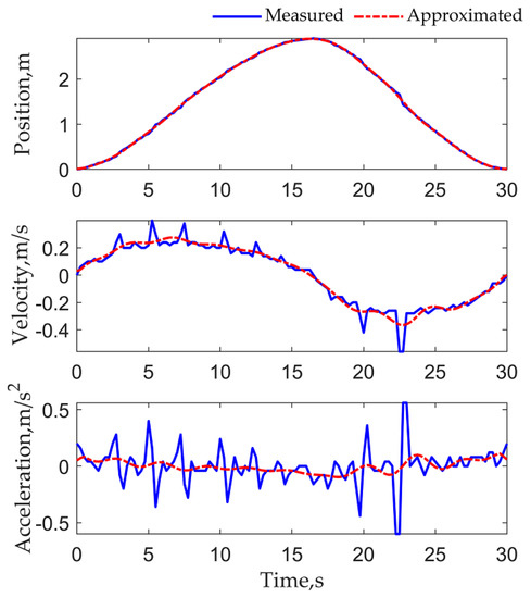
Figure 11.
Measured and approximated polished rod position, velocity, and acceleration.
The motor is Y250M-12 with nameplates parameters PH = 22 kW, nH = 485 rpm, λk = 2.0, ηH = 93.0%. Since iMB is 0.037, the crank velocity can be calculated according to Equations (28) and (33) with the above nameplate parameters. Figure 12 shows the crank angle and acceleration can be obtained by integrating and differentiating the crank velocity.
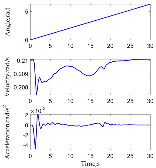
Figure 12.
Calculated crank angle, velocity, and acceleration.
Now the series data for size identification, PR(t), vR(t), aR(t), θ(t), (t), and (t) have been obtained.
According to the polished rod position in Figure 10, it has the values of λ1 and λ2 after solving Equation (36) with the fminunc function of MATLAB. Then, the initial value, lower boundary, and up boundary can be calculated according to Equations (38) and (40) as follows
According to the differences between the measured and the approximated data shown in Figure 11, the noise covariances of the polished rod position, velocity, and acceleration can be obtained with the var function of MATLAB, that is, Rp is 0.0003, Rv is 0.0022 and Ra is 0.0233.
When Qc = 10−7I5, Rc = RvI5, and P00 = 0.15I5, the size of the four-bar linkage can be identified according to the Algorithm 1. The results are shown in Table 6. As is shown in Table 6, the maximum error is 7.09% and the minimum error is −0.15%, which indicates the identified results are accurate. To illustrate the effect of the measured covariances, the size is identified when the measured covariance is Rp, Ra, and Rm respectively. Rm is given by . The results are also presented in Table 6. As can be seen from Table 6, the identified size error of Rp is not the smallest although its value is the smallest, and the error of Rm is the largest because it is a local optimum value. The results indicate that the covariance of the polished rod velocity is appropriate when the covariances of the polished rod position, velocity, and acceleration are different. The reason may be that the noise of the polished rod velocity and acceleration is different from Gaussian noise, and further research is underway.

Table 6.
Real and identified values of size identification with different measurement covariances.
To illustrate the effect of the identified results on the polished rod position, Figure 13 shows the measured, real, and identified polished rod positions, in which the real polished rod position is calculated according to the real size values while the identified one is calculated according to the identified size values. As is illustrated in Figure 13, the identified polished rod position is consistent with the real one while the measured polished rod position is different from the real one, which indicates that the algorithm converges to the real polished rod position rather than the measured one.
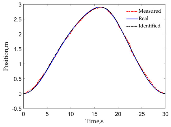
Figure 13.
Measured, real, and identified polished rod position.
5. Results Discussion
5.1. Summary of Obtained Results
In this paper, the four-bar linkage size of the beam pumping units is identified based on the simulated data and the measured data. The obtained results are summarized are as following:
- (1)
- To obtain the crank kinematic data, a speed model of a motor is established according to the Thevenin equivalent circuit of a motor. The validation results indicate that the model is effective. The speed of the motor and the crank kinematic data can be calculated according to the nameplate parameters and the input power of the motor, which is convenient in engineering practice.
- (2)
- To obtain the initial value and the boundary conditions of the size identification, an initial value model is established based on the crank slider mechanism and the relative size restrictions of the beam pumping unit. The validation results based on simulated data show that the model is feasible, which is of great importance to the size identification.
- (3)
- To avoid the arccosine operation due to the inappropriate initial value in the model, a NCCKF algorithm is proposed. The predicted state among the ordinary CKF algorithm should be checked and then modified by solving the constrained optimization problem. The validation results based on simulated data show that the algorithm is feasible but may converge to a local optimum value rather than the real value due to the inappropriate initial value. Therefore, the initial value model is necessary.
- (4)
- To identify the four-bar linkage of a beam pumping unit, a comprehensive size identification algorithm based on the motor input power and the polished rod position is proposed. The identified results based on the simulated data show that the identified sizes can be from the initial values to the corresponding real values within the first 10 s. With the increase in the measurement covariance, the accuracy of identification decreases. The method to obtain the measured noise covariance of the polished rod kinematic data is proposed, and the calculated results demonstrate that the noise covariances of the polished rod position is minimum and that of the acceleration is maximum. The identified results based on the measured data show that the identified result is the most accurate only when the noise covariance of polished rod velocity is utilized.
5.2. Comparison of Different Methods
To better show the advantages of the proposed algorithm, a comparison with several current identification methods is performed. The identification method is RLS method [49], EKF [50], UKF [32,51], and RGD method [52], respectively. The needed data are for Section 4.4 and the measured covariance is Rv. In the method of RLS, EKF, and RGD, the Jacobian matrix is obtained through the complex step differentiation [53]. In RGD method, the information vector is derived from the Jacobian matrix and . In the method of UKF, .
The comparison results are shown in Table 7. For comparison purpose, the results of the proposed algorithm are also listed in Table 7. The mean error in Table 7 denotes the mean value of the absolute error of different methods.

Table 7.
Comparison of different methods.
From the results in Table 7, it can be concluded that the proposed algorithm in the paper is superior in accuracy to the existing methods.
6. Conclusions
The present paper proposed a size identification algorithm of the four-bar linkage of a beam pumping unit based on the nonlinear constrained Cubature Kalman filter. According to the measured motor input power, the crank angle, velocity, and acceleration can be calculated from the speed model of the motor. The initial value, lower boundary, and upper boundary can be obtained by the measured polished rod position based on the initial value model. According to the measured polished rod position, velocity, and acceleration, the four-bar linkage size is identified by the kinematics model of a beam pumping unit, the state space model and the Cubature Kalman filter algorithm. The size identification algorithm is validated based on simulated and measured data, and the identification characteristics under different measurement covariance are studied. The results show that the established models and algorithm are feasible. The identified results based on the simulated data show that the maximum relative error between the identified sizes and the real sizes increases from 0.23% to 9.37% with the covariance increasing from 10−6 to 10−1. The identified results based on the measured oilfield data indicate that the maximum relative error between the identified sizes and the actual sizes is 7.09% when the optimal covariance–that is, the measured covariance of the polished rod velocity–is applied. A comparison with several current identification methods indicates the proposed algorithm in the paper is superior in accuracy. Therefore, the designed soft method can be employed in practical applications. It provides essential services for the future intelligent diagnosis and control of the beam pumping units.
Author Contributions
Conceptualization, J.Y.; methodology, J.Y.; software, J.Y.; validation, J.Y.; formal analysis, J.Y.; investigation, J.Y.; resources, D.S.; data curation, D.S.; writing—original draft preparation, J.Y.; writing—review and editing, J.Y.; visualization, J.Y.; supervision, J.Y.; project administration, H.M.; funding acquisition, H.M. All authors have read and agreed to the published version of the manuscript.
Funding
This research was supported by the Shandong province Natural Science Foundation of China (Grant No. ZR2021MD067), the Fundamental Research Funds for the Central Universities (Grant No. 22CX03011A).
Data Availability Statement
Not applicable.
Conflicts of Interest
The authors declare no conflict of interest.
References
- Zhang, C.; Wang, L.; Wu, X.; Gao, X. Performance analysis and design of a new-type wind-motor hybrid power pumping unit. Electr. Power Syst. Res. 2022, 208, 107931. [Google Scholar] [CrossRef]
- Song, C.; Liu, S.; Han, G.; Zeng, P.; Yu, H.; Zheng, Q. Edge Intelligence Based Condition Monitoring of Beam Pumping Units under Heavy Noise in the Industrial Internet of Things for Industry 4.0. IEEE Internet Things 2022, 1. [Google Scholar] [CrossRef]
- Xu, J.; Meng, S.; Li, W.; Wang, Y. Positive Torque Modulation Method and Key Technology of Conventional Beam Pumping Unit. Energies 2022, 15, 3141. [Google Scholar] [CrossRef]
- Takács, G. A critical analysis of power conditions in sucker-rod pumping systems. J. Pet. Sci. Eng. 2022, 210, 110061. [Google Scholar] [CrossRef]
- Han, Y.; Song, X.; Li, K.; Yan, X. Hybrid modeling for submergence depth of the pumping well using stochastic configuration networks with random sampling. J. Pet. Sci. Eng. 2022, 208, 109423. [Google Scholar] [CrossRef]
- Yibao, C.; Jianfu, L. Optimum design of four-bar linkage of beam-pumping unit based on sensitivity analysis. In Proceedings of the 2010 International Conference on Logistics Systems and Intelligent Management (ICLSIM), Harbin, China, 9–10 January 2010; pp. 503–507. [Google Scholar] [CrossRef]
- Svinos, J. Exact kinematic analysis of pumping units. In Proceedings of the SPE Annual Technical Conference and Exhibition, San Francisco, CA, USA, 5–8 October 1983. [Google Scholar] [CrossRef]
- Feng, Z.-M.; Tan, J.-J.; Li, Q.; Fang, X. A review of beam pumping energy-saving technologies. J. Pet. Explor. Prod. Technol. 2017, 8, 299–311. [Google Scholar] [CrossRef]
- Deshi, Z. Study of power balance technology on beam pumping unit. In Proceedings of the 2013 2nd International Conference on Measurement, Information and Control, Harbin, China, 16–18 August 2013; pp. 1324–1327. [Google Scholar] [CrossRef]
- Zuo, J.; Wu, Y.; Wang, Z.; Dong, S. A Novel Hybrid Method for Indirect Measurement Dynamometer Card Using Measured Motor Power in Sucker Rod Pumping System. IEEE Sens. J. 2022, 22, 13971–13980. [Google Scholar] [CrossRef]
- Hao, D.; Gao, X. Multi-Weighted Partial Domain Adaptation for Sucker Rod Pump Fault Diagnosis Using Motor Power Data. Mathematics 2022, 10, 1519. [Google Scholar] [CrossRef]
- Hao, D.; Gao, X. Unsupervised Fault Diagnosis of Sucker Rod Pump Using Domain Adaptation with Generated Motor Power Curves. Mathematics 2022, 10, 1224. [Google Scholar] [CrossRef]
- Tan, C.; Feng, Z.-M.; Liu, X.; Fan, J.; Cui, W.; Sun, R.; Ma, Q. Review of variable speed drive technology in beam pumping units for energy-saving. Energy Rep. 2020, 6, 2676–2688. [Google Scholar] [CrossRef]
- Sun, J.; Huang, Z.; Zhu, Y.; Zhang, Y. Real-time kinematic analysis of beam pumping unit: A deep learning approach. Neural Comput. Appl. 2022, 34, 7157–7171. [Google Scholar] [CrossRef]
- Min, G.; Chen, C.L.P.; Guang-Yong, C.; Long, C. On Some Separated Algorithms for Separable Nonlinear Least Squares Problems. IEEE Trans. Cybern. 2018, 48, 2866–2874. [Google Scholar] [CrossRef]
- Ding, F.; Zhang, X.; Xu, L. The innovation algorithms for multivariable state-space models. Int. J. Adapt. Control 2019, 33, 1601–1618. [Google Scholar] [CrossRef]
- Li, M.; Liu, X. Maximum likelihood hierarchical least squares-based iterative identification for dual-rate stochastic systems. Int. J. Adapt. Control 2020, 35, 240–261. [Google Scholar] [CrossRef]
- Lian, C.; Xiao, F.; Liu, J.; Gao, S. Parameter and VSI Nonlinearity Hybrid Estimation for PMSM Drives Based on Recursive Least Square. IEEE T. Transp. Electr. 2022, 1. [Google Scholar] [CrossRef]
- Mahadi, M.; Ballal, T.; Moinuddin, M.; Al-Saggaf, U.M. A Recursive Least-Squares with a Time-Varying Regularization Parameter. Appl. Sci. 2022, 12, 2077. [Google Scholar] [CrossRef]
- Ye, Y.; Li, Z.; Lin, J.; Wang, X. State-of-charge estimation with adaptive extended Kalman filter and extended stochastic gradient algorithm for lithium-ion batteries. J. Energy Storage 2022, 47, 103611. [Google Scholar] [CrossRef]
- Jing, S. Multierror stochastic gradient algorithm for identification of a Hammerstein system with random noise and its application in the modeling of a continuous stirring tank reactor. Optim. Contr. Appl. and Met. 2021, 1–13. [Google Scholar] [CrossRef]
- He, Q.; Stinis, P.; Tartakovsky, A.M. Physics-constrained deep neural network method for estimating parameters in a redox flow battery. J. Power Sources 2022, 528, 231147. [Google Scholar] [CrossRef]
- Cui, Z.; Wang, L.; Li, Q.; Wang, K. A comprehensive review on the state of charge estimation for lithium-ion battery based on neural network. Int. J. Energy Res. 2021, 46, 5423–5440. [Google Scholar] [CrossRef]
- Saab, S.S.; Kaed-Bey, R.A. Parameter identification of a DC motor: An experimental approach. In Proceedings of the ICECS 2001. 8th IEEE International Conference on Electronics, Circuits and Systems (Cat. No.01EX483), Malta, Malta, 2–5 September 2001; pp. 981–984. [Google Scholar] [CrossRef]
- Zhu, Z.Q.; Liang, D.; Liu, K. Online Parameter Estimation for Permanent Magnet Synchronous Machines: An Overview. IEEE Access 2021, 9, 59059–59084. [Google Scholar] [CrossRef]
- Kou, B.; Ren, D.; Guo, S. Geometric Parameter Identification of Medical Robot Based on Improved Beetle Antennae Search Algorithm. Bioengineering 2022, 9, 58. [Google Scholar] [CrossRef] [PubMed]
- Ji, Y.; Kang, Z. Three-stage forgetting factor stochastic gradient parameter estimation methods for a class of nonlinear systems. Int. J. Robust Nonlin. 2020, 31, 971–987. [Google Scholar] [CrossRef]
- Kandidayeni, M.; Macias, A.; Amamou, A.A.; Boulon, L.; Kelouwani, S.; Chaoui, H. Overview and benchmark analysis of fuel cell parameters estimation for energy management purposes. J. Power Sources 2018, 380, 92–104. [Google Scholar] [CrossRef]
- Li, Q.; Li, R.; Ji, K.; Dai, W. Kalman Filter and Its Application. In Proceedings of the 2015 8th International Conference on Intelligent Networks and Intelligent Systems (ICINIS), Tianjin, China, 1–3 November 2015; pp. 74–77. [Google Scholar] [CrossRef]
- Kalman, R.E. A new approach to linear filtering and prediction problems. J. Basic Eng. 1960, 82, 35–45. [Google Scholar] [CrossRef]
- Bellantoni, J.; Dodge, K. A square root formulation of the Kalman-Schmidt filter. AIAA J. 1967, 5, 1309–1314. [Google Scholar] [CrossRef]
- Kolås, S.; Foss, B.A.; Schei, T.S. Constrained nonlinear state estimation based on the UKF approach. Comput. Chem. Eng. 2009, 33, 1386–1401. [Google Scholar] [CrossRef]
- Fujii, K. Extended Kalman Filter; Refernce Manual. 2013, pp. 14–22. Available online: https://www-jlc.kek.jp/2004sep/subg/offl/kaltest/doc/ReferenceManual.pdf (accessed on 20 July 2021).
- Moradkhani, H.; Sorooshian, S.; Gupta, H.V.; Houser, P.R. Dual state–parameter estimation of hydrological models using ensemble Kalman filter. Adv. Water Resour. 2005, 28, 135–147. [Google Scholar] [CrossRef]
- Julier, S.J.; Uhlmann, J.K.; Durrant-Whyte, H.F. A new approach for filtering nonlinear systems. In Proceedings of the 1995 American Control Conference-ACC’95, Seattle, WA, USA, 21–23 June 1995; pp. 1628–1632. [Google Scholar] [CrossRef]
- Safarinejadian, B.; Vafamand, N. Kalman Randomized Joint UKF Algorithm for Dual Estimation of States and Parameters in a Nonlinear System. J. Electr. Eng. Technol. 2015, 10, 1212–1220. [Google Scholar] [CrossRef]
- Arasaratnam, I.; Haykin, S. Cubature Kalman Filters. IEEE Trans. Autom. Control 2009, 54, 1254–1269. [Google Scholar] [CrossRef]
- Zarei, J.; Shokri, E. Nonlinear and Constrained State Estimation Based on the Cubature Kalman Filter. Ind. Eng. Chem. Res. 2014, 53, 3938–3949. [Google Scholar] [CrossRef]
- Simon, D. Kalman filtering with state constraints: A survey of linear and nonlinear algorithms. IET Control Theory A 2010, 4, 1303–1318. [Google Scholar] [CrossRef]
- Rajput, S.; Farber, E.; Averbukh, M. Optimal Selection of Asynchronous Motor-Gearhead Couple Fed by VFD for Electrified Vehicle Propulsion. Energies 2021, 14, 4346. [Google Scholar] [CrossRef]
- Averbukh, M.; Lockshin, E. Estimation of the Equivalent Circuit Parameters of Induction Motors by Laboratory Test. Machines 2021, 9, 340. [Google Scholar] [CrossRef]
- Adekitan, A.I. Supply instability induced torque variations of a three phase asynchronous motor. Int. J. Mech. Eng. Tech. 2018, 9, 572–583. Available online: https://www.iaeme.com/ijmet/issues.asp?JType=IJMET&VType=9&IType=6 (accessed on 1 June 2018).
- He, J.; Ji, K.; Xu, M.; Mei, G.; Lin, D.; Xia, H. Analysis of variable frequency energy-saving operation of beam pumping unit. IOP Conf. Ser. Mater. Sci. Eng. 2018, 452, 042185. [Google Scholar] [CrossRef]
- Wang, B. Design and Calculation of Oil Production Machinery; Petroleum Industry Press: Beijing, China, 1998; pp. 39–41. [Google Scholar]
- Dong, S.; Zhang, S. Pumping Design Calculations and Computer-Implemented; Petroleum Industry Press: Beijing, China, 1994; pp. 73–75. [Google Scholar]
- Li, H.; Sun, H.; Chen, B.; Shen, H.; Yang, T.; Wang, Y.; Jiang, H.; Chen, L. A cubature Kalman filter for online state-of-charge estimation of lithium-ion battery using a gas-liquid dynamic model. J. Energy Storage 2022, 53, 105141. [Google Scholar] [CrossRef]
- Simon, D.; Chia, T.L. Kalman filtering with state equality constraints. IEEE Trans. Aerosp. Electron. Syst. 2002, 38, 128–136. [Google Scholar] [CrossRef]
- Yin, J.-J.; Sun, D.; Yang, Y.-S. Predicting multi-tapered sucker-rod pumping systems with the analytical solution. J. Pet. Sci. Eng. 2021, 197, 108115. [Google Scholar] [CrossRef]
- Rahrooh, A.; Buchanan, W.W.; Seker, R. Linear Model Estimation of Nonlinear Systems Using Least-Squares Algorithm5. In Proceedings of the 120th ASEE Annual Conference & Exposition, Atlanta, GA, USA, 23–26 June 2013; Available online: https://commons.erau.edu/publication/1257 (accessed on 25 November 2022).
- Silvestrini, S.; Piccinin, M.; Zanotti, G.; Brandonisio, A.; Lunghi, P.; Lavagna, M. Implicit Extended Kalman Filter for Optical Terrain Relative Navigation Using Delayed Measurements. Aerospace 2022, 9, 503. [Google Scholar] [CrossRef]
- Van Der Merwe, R. Sigma-Point Kalman Filters for Probabilistic Inference in Dynamic State-Space Models. Ph.D. Thesis, Oregon Health and Science University, Portland, OR, USA, 2004. [Google Scholar]
- Wang, Y.; Ding, F. Recursive least squares algorithm and gradient algorithm for Hammerstein–Wiener systems using the data filtering. Nonlinear Dynam. 2015, 84, 1045–1053. [Google Scholar] [CrossRef]
- Lai, K.L.; Crassidis, J.L. Extensions of the first and second complex-step derivative approximations. J. Comput. Appl. Math. 2008, 219, 276–293. [Google Scholar] [CrossRef]
Publisher’s Note: MDPI stays neutral with regard to jurisdictional claims in published maps and institutional affiliations. |
© 2022 by the authors. Licensee MDPI, Basel, Switzerland. This article is an open access article distributed under the terms and conditions of the Creative Commons Attribution (CC BY) license (https://creativecommons.org/licenses/by/4.0/).