Article

Development of the Cost-Based Model for Monitoring the Lifetime of the Earth Moving Machines

1
Faculty of Mechanical Engineering, University of Belgrade, 11120 Belgrade, Serbia
2
Faculty of Mining and Geology, University of Belgrade, 11120 Belgrade, Serbia
*
Author to whom correspondence should be addressed.
Machines 2022, 10(11), 995; https://doi.org/10.3390/machines10110995
Submission received: 20 August 2022 / Revised: 14 October 2022 / Accepted: 26 October 2022 / Published: 29 October 2022
(This article belongs to the Section Machines Testing and Maintenance)

Abstract

:
This paper presents the model for the identification of reference points on the lifetime curve of engineering systems. This curve commonly represents the increase and decline of failure in relation to time. A direct correlation between failure rate and costs is assumed in this paper, therefore, statistical and empirical analysis of costs provided reference points. This approach is used for positioning stages of the engineering system’s lifetime with a minimal number of failures and costs, regardless of whether these are acceptable or not. The following three stages are usually identified: the beginning, the stationary part and the end of life. The boundaries between them are recognized on the basis of minimum total lifetime costs and on economic lifetime costs. Model is tested on the dozers, machines frequently used in the mining industry for the earthmoving operations, and which are characterized by high operating and maintenance costs.

1. Introduction

Successful management of an engineering system’s lifetime has the task of reducing costs and maximizing profit while achieving required production rates and preserving the status of equipment and machines. Equipment is passed through several stages of its lifetime during the operation, which can be defined according to different criteria in function to the purpose of the equipment. In function of time, equipment is inevitably getting old, with an increasing number of failures and decreasing availability. Reduced availability is generating additional operational and maintenance costs, reducing the profit further [1]. The relation between increasing costs and time, i.e., the age of equipment, is evident [2].
It is important for the owner of the equipment to identify the reference points between the lifetime stages of the engineering system or the machine. The property of these stages is the level of cost, which can be minimal, acceptable, or unacceptable [3]. The major task here is to determine the maximal profit and to establish an acceptable level of cost for the owner, i.e., to identify the specific period of the machine’s lifetime [4]. The International Electrotechnical Commission (IEC) presented the Dependability management: Application guide—Life cycle costing (IEC 60300-3-3:2017 and 2018) standard [5]. The purpose of this standard is to provide basic guidelines for the assessment of dependability and costs, including cost determination in relation to the quality of service [5] of the engineering system. The systemic approach is necessary to define the ownership and operational costs, which include acquisition, maintenance, operation, overhaul, etc. This approach also requires a certain balancing level between the costs and the residual value of the machine [2]. This balance is achieved by assessing the dependability trend against costs induced by the analyzed system at any given time of its life [1].
In general, there are several lifetime stages of an engineering system or equipment [1]. A technical lifetime is a period during which the equipment meets the designed criteria and guaranteed production rates [4,6]. An economic lifetime is a period defined by the depreciation of investment, i.e., the comparison of net present value, future expenses and income [6]. An economic lifetime is usually shorter than a technical lifetime, and it also requires investment in the refurbishment of the equipment [4,6]. A licensed lifetime is defined by the approval for operation or changes in legislation related to this approval. Technological lifetime is related to the obsolescence of incorporated technology, and it can be extended by modernization, reconstruction, or revitalization through investment [4,6].
Regarding the analysis of the machine’s lifetime stages, the economic lifetime is the most relevant since it includes the costs. The basic classification of costs related to the machines divides these into direct and indirect costs [4]. Indirect costs are generated due to the machine’s failure. The unreliable machine generates stoppages in the production process, where the failure of one machine frequently causes a standstill in the operation of other machines. No production is achieved during the failure of the machine, hence the indirect costs. Direct costs are easy to measure. These are created by the acquisition of the machine (buying), the operation of the machine and necessary maintenance. Operational costs are diversified. These are related to numerous parameters of economical and technical nature. Size and the structure of the costs are also related to equipment ownership. The following three models of equipment ownership are common [2,6]:
  • In the first model, the company operates its equipment or part of it and takes care of it. The advantage of this model is that a company can manage and optimize the costs in relation to time, unify the fleet, implement its own maintenance policy and reduce operational costs that are generated only during the operation of the machine;
  • In the second model, equipment is rented from a subcontractor specialized for the task at hand. In this case, the costs are fixed regardless of the age of the machine. The company does not have to organize the maintenance. The disadvantage of this model is that costs are incurred regardless of whether the machine is operating or not. Namely, in addition to the costs of active work, the costs of passive engagement are also generated since the machine cannot be engaged with another company during the time defined by the contract;
  • The third model is a combination of the previous two models, where the company owns the equipment while the specialized subcontractor is engaged in the maintenance.
For the purpose of quality asset management, it is relevant to monitor the costs incurred by the equipment, as well as to define the criteria and boundaries between the ownership types, i.e., the way the equipment is used. The company must provide clear answers to the questions of what the largest profit is, what the realistic profit is, and whether the ownership costs are smaller, equal, or larger than the costs of renting the same equipment. This is the basis for making the conclusion about buying or renting the equipment.
The analysis performed in this paper is focused on the following previously mentioned terms: costs and lifetime. The case study is based on auxiliary mining machines, operating in the lignite open pits—dozers. Dozers are the most numerous and frequently used pieces of auxiliary mechanization, with the largest number of tasks [7]. Dozers operating on the large lignite open pits have the task of completing in-time and quality work related to auxiliary operations [2]. This approach provides the optimal operating conditions for capital mining equipment, while simultaneously securing better safety for both the workers and the equipment [8]. Direct costs are accepted as an economic indicator for successful operation since the dozers are not generating direct profit for the owner. The analysis included two different manufacturers of the dozers, which are operating in somewhat equal conditions and at the same time intervals. The goal of this research is to establish the costs incurred by these machines in the function of time. The final output is to identify the two reference points also in function of time (years of age) to obtain the three stages of the machine’s lifetime.
Such analysis with the purpose of machine lifetime management is important due to the difficult operating conditions. As a starter, the acquisition of mining mechanization is a large investment. The operation of these machines is demanding, with high risk involved. Machines are operating at varying operational and climate conditions, with a lot of uncertainty involved in relation to maintenance and intense demands to repair them as soon as possible, etc. Some previous research indicates that one hour of an unplanned stoppage at a continuous lignite mining system incurs costs on the order of several tens of thousands of Euros [7,9,10].
Earthmoving machines, such as dozers, have their own specifics as follows: they are produced in large series, they usually work during the whole year, and they have quality maintenance while they are new and in the warranty period [2,6]. This is appropriately reflected in the lifetime costs and the failure rate, which are described in this article.
This paper provides the model for monitoring the costs that enables the capability to identify the moment when the owner’s profit starts to decline and the moment until it is acceptable for the owner to use their own machines instead of rented ones. In this way, the boundary within the lifetime of the machine is established.

2. Materials and Methods

2.1. Lifetime Stages of the Machines

Lifetime stages and the associated costs are conditioned by failure rate. The relationship between failure rate and operation time is shown in Figure 1. There are three distinct stages, which could somewhat differ depending on the type of the machine and the means of its production [1].
Machine type A (Figure 1A): These machines are manufactured in individual production [1]. The machine is put in operation with numerous weaknesses i.e., insufficiently developed functions and details. At the beginning of the operation, these mistakes are manifested as so-called infant mortality. Failure rate and belonging costs are high with a declining trend (stage I). According to the feedback from the operator and the maintenance, weaknesses are repaired and the machine transits into the stationary regime of operation (stage II). During this stage failure rate is reduced and constant while the costs are low with a slightly increasing trend. Toward the end of the machine’s lifetime (stage III) it transits into the stage of increased failure rate and significant rise in costs. This interpretation of the failure rate is commonly called the bath-tub curve.
Machine type B (Figure 1B): These machines are manufactured in serial production. A high failure rate (infant mortality) appears only during the prototype development of the machine. Machines manufactured for the sale do not have initial and sudden failures. Failures are very rare during the first stage of the lifetime as well as belonging costs. The remaining stages are identical to machine type A.
Machines type A are huge mining and energetics plants, stationary transport systems and similar. Machines type B are more common machines such as vehicles, power transmission boxes, devices and apparatus. For both types of machines overview of failure rate and cost in different stages of a lifetime is presented in Table 1. The subject of analysis in the paper is machines from the group type B, which are more widely distributed in the industry.
As described above, it is difficult to identify the moment of transition from one stage into the other. It is evident that trends in failure and the level of costs are changing at the transition points. The purpose of the cost analysis model is to define the reference points as delimitators of the machine’s lifetime stages in relation to costs as a function of time. The first reference point or transition point from stage I into stage II of the lifetime is the economic lifetime with maximal profit (as called in this paper), which is the moment when the machine no longer achieves the maximum possible increase in income. The second reference point or transition point from stage II into stage III of the lifetime represents the economic life of the technical system, which is established as the moment when costs incurred by the operation of the machine surpass the renting costs of the suitable machine [6].

2.2. Machine’s Operational Costs

In article [11] internal costs of engineering systems are divided into the following five categories: value depreciation, operating cost, fixed cost, repairs and maintenance, and other costs. This approach is typical for vehicles. Article [7] suggests that technological process costs are defined by production losses generated from failures, and by operational and maintenance costs. Some manufacturers developed their methodology for assessing the quality of service and the machine’s remaining capabilities. The cost calculation algorithm is one of the integral components of these methodologies. Commonly used approaches in the mining industry are developed by two manufacturers, Caterpillar and Komatsu. Caterpillar developed a methodology for its product line, and it is an algorithm for the calculation of ownership costs and operational costs [12]. The methodology by Komatsu is more focused on the replacement intervals [13]. Both methodologies are essentially using the same cost structure. The usual approach in practice is to adjust mentioned models/methodologies to the specific operating conditions to create a more specific cost determination method. As mentioned earlier, the case study in this paper is based on the analysis of dozers operating on lignite open pits [2,6,7,8,12,13,14]. Dozer’s costs are comprised of ownership costs, operational costs and labor costs. Individually, these costs can be represented as follows [1,2,8]:
  • Ownership costs: equipment depreciation and insurance;
  • Operational costs: energy, lubricants, wearing parts, maintenance and other specific costs;
  • Labor costs: operators and maintenance staff.

2.2.1. Total and Specific Costs

Costs can be presented as cumulative costs and as a specific value. Specific costs are obtained with their expression by working or operating hours of the machine. Unit for specific cost is cost value per working hour [EUR/wh]. This approach provides the values which can be compared for different machines.
Input data for calculation of dozer’s ownership costs are purchase price, depreciation period, the current age of the machine in years and total/cumulative number of operating hours. The accepted value for the depreciation period (B) is 10 years, which is a typical period for dozers operating on lignite open pits. Depreciation for each operating hour is calculated by dividing the purchase price by the total number of operating hours of the machine in the analyzed period. For machines operating N years, where N < B = 10 years, Equation (1) is used with annual depreciation coefficient of a = 1/B = 1/10 = 0.1. Purchase price K is in this way reduced to the value Kr [EUR] [2,6].
K r = 1 B N a K
The second part of ownership costs are insurance costs, which are calculated according to the Equation (2) as follows [15]:
I = K N + 1 + S N + 1 2 N i 100 C
where I is specific insurance costs [EUR/wh]; S—the residual value of the machine at the time of replacement (resale value) [EUR]; C—average annual utilization of machine [wh/y]; i—insurance coefficient.
Operational costs are including the consumption of energy (fuel), lubricants, wear parts and maintenance. There are two approaches to calculating these costs. The first one is used when cumulative costs are known for a certain period of operation as well as incurred working hours. Specific costs are calculated by dividing the costs by working hours. The second approach is used when the specific consumption of materials and supplies is known. In this case, operational costs are calculated by multiplying the number of consumed materials and supplies with their unit price [15]. The first approach will be used in the case study in this paper.
Input data for calculating labor costs for operating the machine are the overall number of workers, gross salary of workers, number of machines, number of operating teams, coefficient of the reserve, etc. Input data for calculating labor costs for maintenance in a specific period are the number of interventions, total operation time of the machines, number of services, the overall number of workers, gross salaries, etc.

2.2.2. Determination of Costs Function

The costs are changing in time with the age of the machine. Therefore, costs can be expressed as a time-dependent function [16].
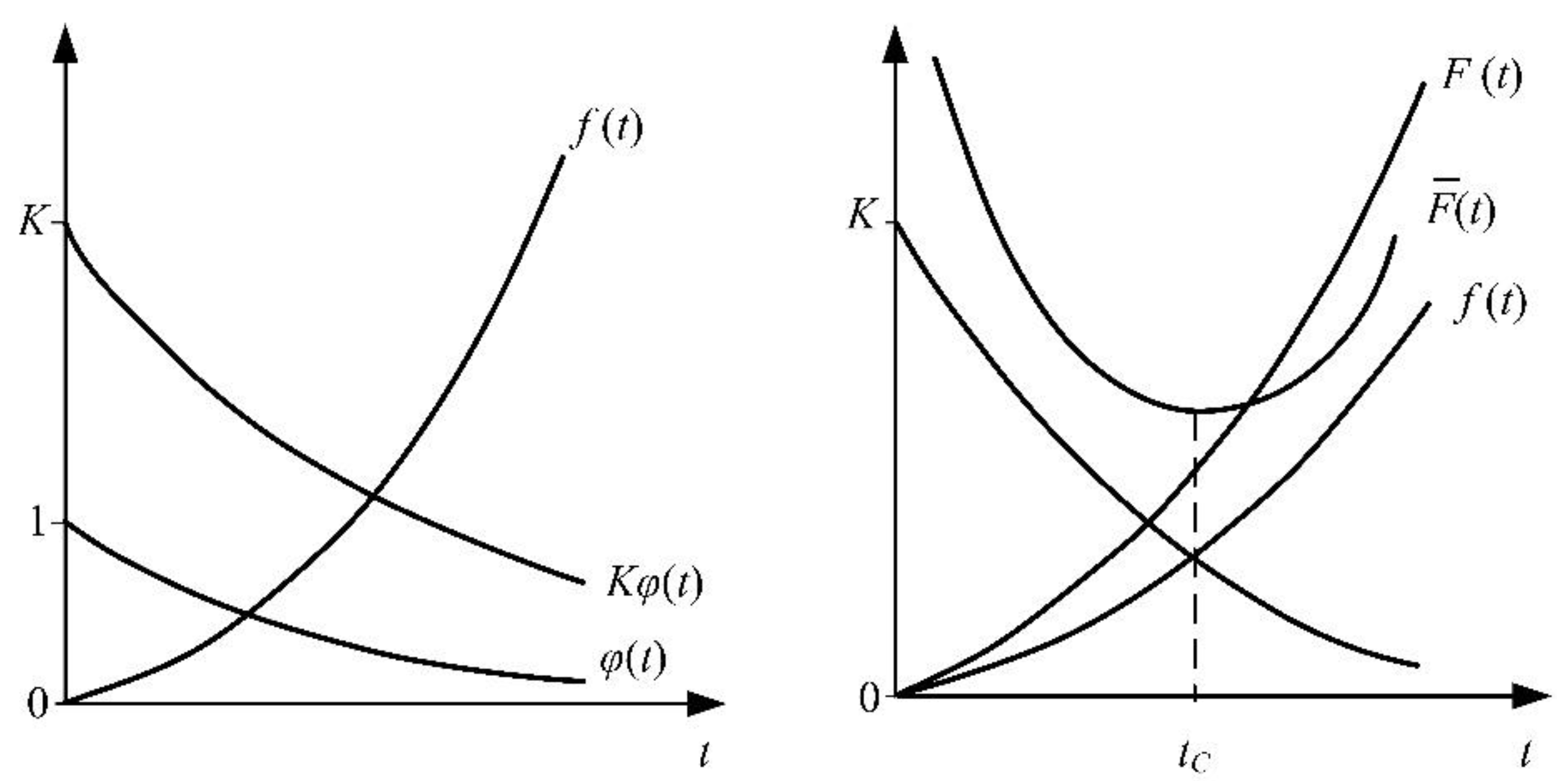
Assume the machine acquired at moment t = 0 at purchase price K. Value of the machine is reduced and φ(t) represents the write-off coefficient of the machine’s value. The value of the machine after time t is K·φ(t) [16].
Function φ(t) at the moment t = 0 must be φ(0) = 1 since the machine is brand new and it has the value K. The value of the machine is reduced in time, hence the φ(t) must be a monotonically decreasing function, tending to zero as time passes.
Function f(t) represents cumulative maintenance costs and in moment t = 0 must be f(0) = 0. In time the costs are getting larger hence the f(t) must be a monotonically increasing function. Costs in some time interval (t1, t2) can be obtained as f(t1)–t(t2).
Overall operational costs of the machine are the purchase price of machine K, maintenance costs f(t) reduced by the value of the machine at the moment t as follows:
F ( t ) = K + f ( t ) K φ ( t ) , o r
F ( t ) = K 1 φ ( t ) + f ( t )
F(t) is a monotonically increasing function in time t. Since φ(t) is a monotonically decreasing function always smaller than 1, then 1 − φ(t) is a monotonically increasing function with 1 − φ(0) = 0. Value f(0) = 0 results in F(0) = 0.
When t → ∞ then φ (∞) → 0 i.e., 1 − (∞) → 1 therefore the total operational costs are determined by the purchase price of the machine (Figure 2) [6,16].
Operational costs did not have the extreme since they are described with monotonically increasing function. Due to definition of functions f(t), φ(t) and F(t) the function of average costs F ¯ (t) is convex and defined as follows (Figure 2):
F ¯ = 1 t K 1 φ ( t ) + 1 t f ( t )
Average costs F ¯ (t) will be decreasing function up until the time tC after that the costs will start to increase. The moment t = tC is a time when the average costs in the period [0, tC] are minimal (Figure 2).
The interval period of operation [0, tC] with the minimal average cost is obtained with the first derivative of the function F ¯ (t) as follows:
d F ¯ ( t ) d t = 1 t 2 K φ ( t ) + f ( t ) t K 1 φ ( t ) f ( t ) = 0
The previous equation could have the solution for t = tC, i.e., the average costs shall be minimal if the following conditions are met:
d 2 F ¯ ( t ) d t 2 > 0
This model for the definition of costs function does not include a discount factor since it is based on a partial machine’s write-off.

3. Results—Case Study

The case study incorporates an analysis of costs incurred by dozer operations and the determination of reference points of a lifetime. Dozers are a B-type of machines and they are operating on lignite open pits. The analysis included the following two different dozers: the Caterpillar D8R (type 1) and the Liebherr PR-752/754 (type 2). Dozers are of the same class and are operating in almost similar conditions. The analysis encompassed 15 individual Caterpillar machines and 3 Liebherr machines.

3.1. Data Collection

Information on costs is obtained from internal documentation of EPS [2]. Values of specific costs for ownership costs (OWC), operational costs (OPC), human resource costs-labor costs (HRC) and total costs (TC) are given in Table 2. Costs are presented as average annual specific values [EUR/wh]. Data are given for the initial 10 years of operation.
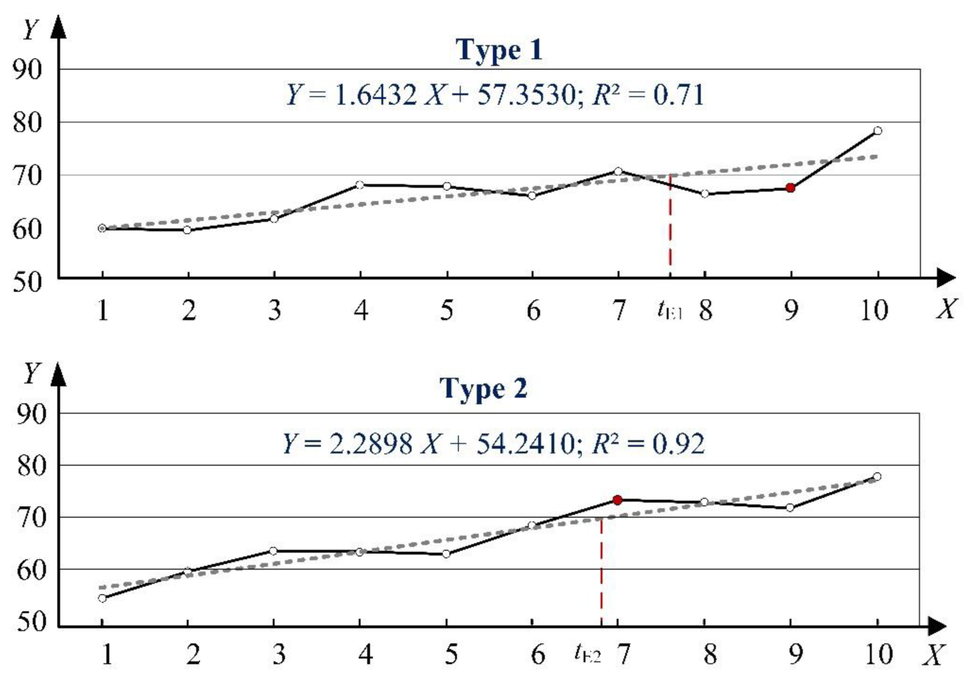
The relationship diagram of specific values of total costs and the age of the machine is shown in Figure 3 (solid line). It can be seen that there is an approximately linear trend of cost increase in relation to the age of machines. The linear approximation of costs was performed with the least square method, which also indicated the trend of increase in time. The equation of line Y = f(X) and Pearson’s correlation coefficient (R2) are also given in Figure 3 (dashed line). The approximation for machine type 1 has a correlation value of R2 in the interval [0.71–0.90], which is, according to [17], a “high” correlation, while for the machine type 2, the value of R2 is in the interval [0.91–1], which is a “very high” correlation. The slope of regression line 1 is smaller compared to line 2 (1.6432 < 2.2898), meaning that the cost increase is slower for machine 1. An occasional drop in operational costs was caused by service investments in machines. The goodness of the linear regression model is verified by using the Kolmogorov–Smirnov goodness of fit test (KS-test) [18]. According to KS-test, the maximum deviation between the data and the linear regression model for machine type 1 is at point 9, while for machine type 2 is at point 7 (marked in Figure 3). Deviations are 0.067 and 0.064, respectively, and are lower than an α-value of 0.41 for a confidence level of 0.95.

3.2. Reference Points of Economic Lifetime (tE)

The criterion for the economic lifetime is that costs induced by the machine are smaller than the cost of renting one at a market price of 70 EUR/wh [2,6]. Equaling the approximated cost’s function (Figure 3) and the stated price for renting the machine provides the solution for the equation as a moment tE in years that represents the profitability limit, i.e., the reference point of economic lifetime.
For the Y = 70 [EUR/wh] and X = tE, we obtain the following:
  • Machine type 1:  70 = 1.64 · tE1 + 57.35 → tE1 = 7.70 years;
  • Machine type 2:  70 = 2.29 · tE2 + 54.24 → tE2 = 6.88 years.

3.3. Reference Points of Minimal Costs Lifetime (tC)

Reference point tC represents the limit of machine operation at minimal average costs. A polynomial function of cumulative maintenance (total) costs f(t) (obtained using MATHEMATICA software [19]), the function of total costs of the machine’s operation F(t), and the function of average costs F ¯ (t) are defined according to the data provided in Table 2.
  • Machine type 1:
f ( t ) = 0.00253 t 7 + 0.08847 t 6 1.17575 t 5 + 7.48052 t 4 24.60580 t 3 + 50.48850 t 2 17.59891 t + 0.08008
F ( t ) = K + f ( t ) K φ ( t ) = 459.95 460 ( 1 0.28460 t 0.5 ) 17.59891 t + 50.48850 t 2 24.60580 t 3 + 7.48052 t 4 1.17575 t 5 + 0.08847 t 6 0.00253 t 7
where: K = 460,000 EUR, φ(t) = 1 − 0.28460 · t0.5 [12,14].
F ¯ ( t ) = 1 t K 1 φ ( t ) + 1 t f ( t ) = 17.59891 + 0.08008 t + 130.9 t 0.5 + 50.48850 t 24.46040 t 2 + 7.48052 t 3 1.17575 t 4 + 0.08847 t 5 0.00253 t 6
Solution for the function’s first derivative, provides the moment tC with minimal average costs.
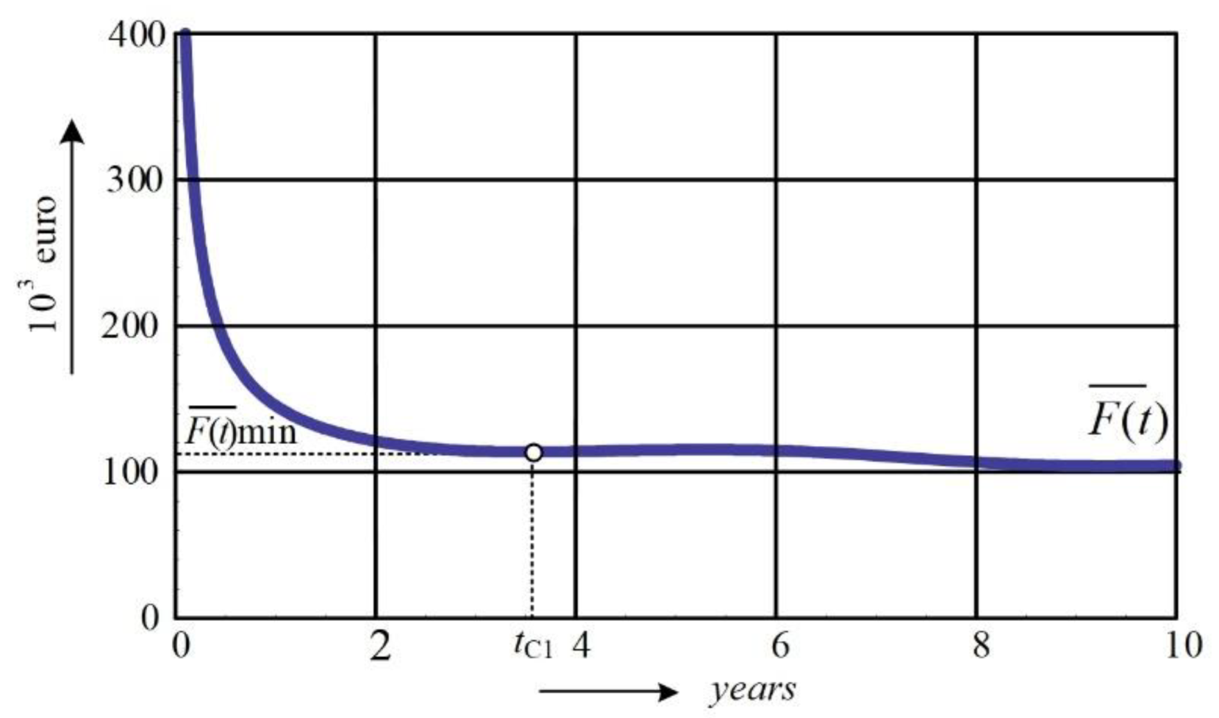
d F ¯ t d t = 1 t 2 K φ t + f t t K 1 φ t f t = 0 50.48850 0.08008 t 2 65.48500 t 1.5 49.21160 t + 22.44160 t 2 4.70300 t 3 + 0.44237 t 4 0.01520 t 5 = 0 t C 1 = 3.5204   y e a r s
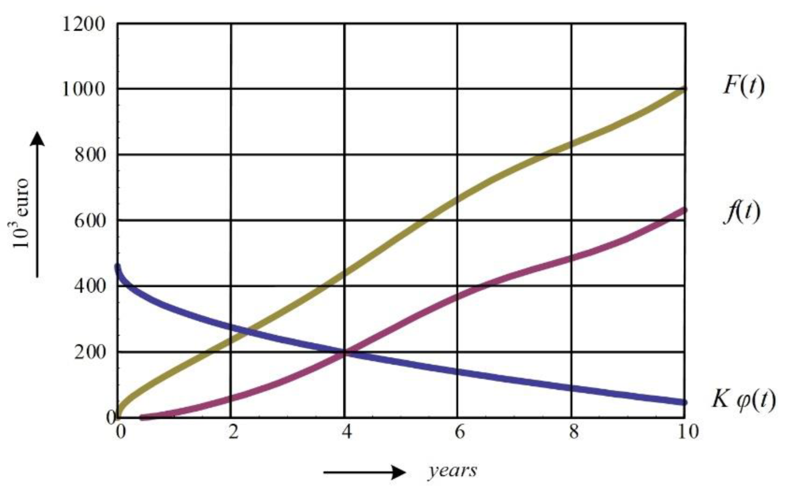
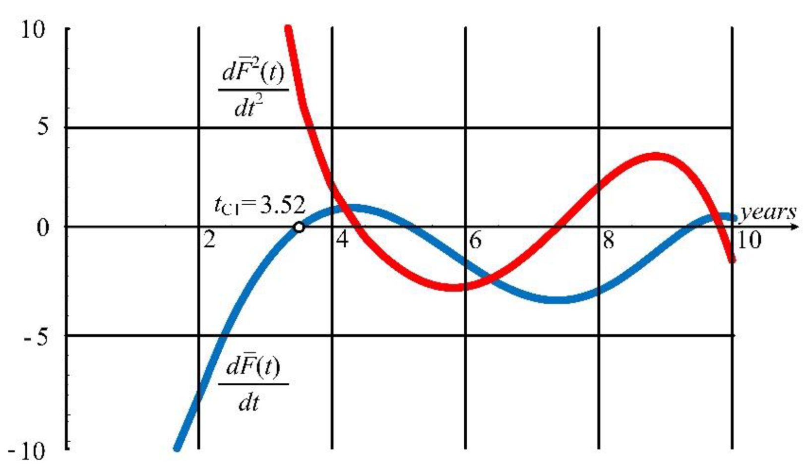
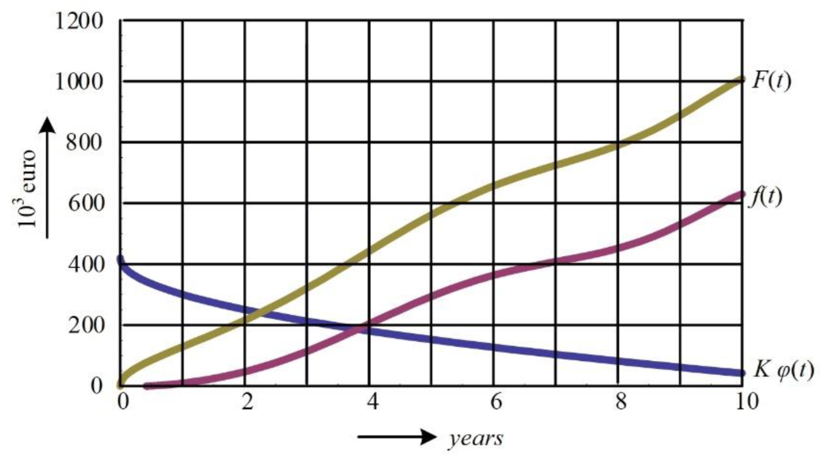
The increasing function of cumulative maintenance (total) costs f(t), the function of total costs of the machine’s operation F(t) and the decreasing function representing the value of the machine at any given time of K·φ(t) are shown in Figure 4. The function of average costs F ¯ (t) for machine type 1 is shown in Figure 5. Differential analysis of the function F ¯ (t) resulted in the moment tC1 = 3.52 years. The first derivative d F ¯ /dt and the second derivative d2 F ¯ /dt2 are shown in Figure 6. The point where function d F ¯ /dt changes sign and function F ¯ (t) has a minimum can be easily identified in the figure.
  • Machine type 2:
The calculation for machine type 2 has been performed on the same principles. A review of calculated values is given respectively below. Moreover, defined functions are presented graphically in the same manner.
f ( t ) = 0.00297 t 7 + 0.09001 t 6 0.98401 t 5 + 4.67785 t 4 10.46040 t 3 + 24.94660 t 2 9.05238 t + 0.02643
F ( t ) = K + f ( t ) K φ ( t ) = 420.026 420 ( 1 0.28460 t 0.5 ) 9.05238 t + 24.94660 t 2 10.46040 t 3 + 4.67785 t 4 0.98401 t 5 + 0.09001 t 6 0.00297 t 7
where: K = 420,000 EUR, φ(t) = 1 − 0.28460 · t0.5 [2,6].
F ¯ ( t ) = 1 t K 1 φ ( t ) + 1 t f ( t ) = 9.05238 + 0.02643 t + 119.5 t 0.5 + 24.94660 t 10.46040 t 2 + 4.67785 t 3 0.98401 t 4 + 0.09001 t 5 0.00297 t 6
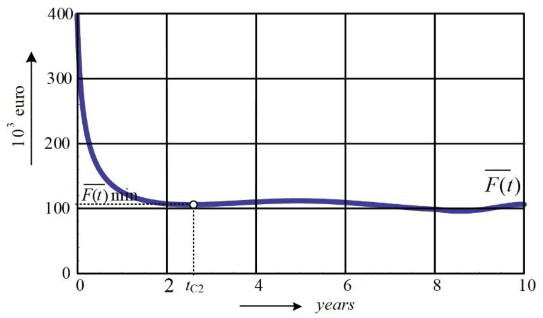
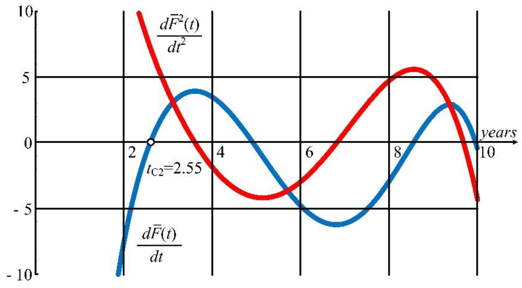
d F ¯ t d t = 1 t 2 K φ t + f t t K 1 φ t f t = 0 24.94660 0.02643 t 2 59.76600 t 1.5 20.92080 t + 14.03360 t 2 3.93604 t 3 + 0.45005 t 4 0.01782 t 5 = 0 t C 2 = 2.5484   y e a r s
Described functions are presented in Figure 7, Figure 8 and Figure 9.

4. Discussion

Reference points of the dozer’s lifetime are defined by calculations, and an overview of the results is presented in Table 3. Transition moments from stage I into II and from stage II into III of the lifetime, for both dozers, are given in the table. As it can be seen, machine type 2 reaches both reference points earlier, with a more significant difference at the transition from stage I into stage II. Moreover, machine type 2 incurs larger costs and deteriorates faster.

5. Conclusions

The lifetime of the engineering system comprises the following three time stages: the start of the operation when the machine is new, normal stationary life that represents the longest period of a lifetime, and the end of the lifetime when the machine suffers from intensive failures and deterioration. Each period has a typical failure rate and induced costs. It is difficult to accurately establish the boundary between these periods. However, it is important for the owner to define the moment of a significant increase in failure rate and associated costs. The possibility of replacing the old machine with a new one should be considered at these moments.
According to empirical data, it is possible to use statistical analysis to establish the failure rate as a function of costs. This calculation is of a high level of confidence during the initial years of operation. As the machine deteriorates, this calculation becomes more difficult due to disturbance values and causes uniformity disorder in the model. Machines manufactured in serial production were analyzed in this paper. It is suggested that the transition from the first into the second stage of the machine’s lifetime should be identified as a minimal cost lifetime. This point represents the moment until which machines generate profit without the cost of unplanned stoppages–failures. The period beyond this point has a slight increase in the machine’s operational costs, up until the economic lifetime point. At this point, the machine transits from the second into the third stage of the lifetime during which the costs of failures are becoming so large that the owner can create more profit by renting a similar machine from the specialized subcontractor.
A case study for this model is presented for the dozers operating in lignite open pits. It has been shown that reference points are not the same for two types of machines from different manufacturers. The first reference point occurs approximately after 3 ± 0.5 years of operation, while the second occurs after 7.2 ± 0.5 years of operation. This analytical approach can be a useful tool for decision-making on the acquisition of similar equipment.
The model from the case study is not universal due to the linear approximation of costs that is characteristic of machines that are constantly working and that are regularly maintained. The model is fully adaptable. It is necessary to adjust the cost function to some other mathematically defined trend line.

Author Contributions

Conceptualization, U.B. and M.T.; methodology, U.B. and M.T.; validation, M.T. and S.D.; formal analysis, S.D. and I.J.; resources D.I.; writing—original draft preparation, S.D. and I.J.; writing—review and editing, U.B. and M.T.; visualization, S.D.; supervision, D.I. All authors have read and agreed to the published version of the manuscript.

Funding

This research received no external funding.

Data Availability Statement

Not applicable.

Conflicts of Interest

The authors declare no conflict of interest.

References

  1. Dhillon, B.S. Mining Equipment Reliability, Maintainability, and Safety; Springer: London, UK, 2008. [Google Scholar]
  2. Optimization of the organization, resources and costs of auxiliary mechanization in order to increase the degree of utilization of tailings and coal systems at the surface mines of electric power industry of serbia. In Study; Faculty of Mining and Geology Belgrade: Belgrade, Serbia, 2018. (In Serbian)
  3. Jagodic-Krunic, D.; Vujic, S.; Tanasijevic, M.; Dimitrijevic, B.; Subaranovic, T.; Ilic, S.; Maksimovic, S. Model Approaches to Life Cycle Assessment of Auxiliary Machines Based on an Example of a Coal Mine in Serbia. J. Min. Sci. 2018, 54, 404–413. [Google Scholar] [CrossRef]
  4. Al-Chalabi, H.; Lundberg, J.; Jonsson, A. Economic lifetime of a drilling machine: A case study on mining industry. Int. J. Strateg. Eng. Asset Manag. 2015, 2, 177–189. [Google Scholar] [CrossRef] [Green Version]
  5. IEC 60300-3-3:2017; Dependability Management—Part 3–3: Application Guide—Life Cycle Costing. The International Electrotechnical Commission: Geneva, Switzerland, 2009.
  6. Janković, I. Optimisation of the Life Cycle concept of Auxiliary Machinery at Lignite Open-pit Mines. Ph.D. Thesis, University of Belgrade, Belgrade, Serbia, 2020. Available online: https://uvidok.rcub.bg.ac.rs/handle/123456789/3788 (accessed on 13 May 2020). (In Serbian).
  7. Bugaric, U.; Tanasijevic, M.; Polovina, D.; Ignjatovic, D.; Jovancic, P. Lost production costs of the overburden excavation system caused by rubber belt failure. Eksploat. I Niezawodn. Maint. Reliab. 2012, 14, 333–341. [Google Scholar]
  8. Jankovic, I.; Djenadic, S.; Ignjatovic, D.; Jovancic, P.; Subaranovic, T.; Ristovic, I. Multi-criteria approach for selecting optimal dozer type in open-cast coal mining. Energies 2019, 12, 2245. [Google Scholar] [CrossRef] [Green Version]
  9. Pantelić, M.; Bošnjak, S.; Misita, M.; Gnjatović, N.; Stefanović, A. Service FMECA of a bucket wheel excavator. Eng. Fail. Anal. 2020, 108, 104289. [Google Scholar] [CrossRef]
  10. Djenadic, S.; Tanasijevic, M.; Jovancic, P.; Ignjatovic, D.; Petrovic, D.; Bugaric, U. Risk Evaluation: Brief Review and Innovation Model Based on Fuzzy Logic and MCDM. Mathematics 2022, 10, 811. [Google Scholar] [CrossRef]
  11. Gössling, S.; Kees, J.; Litman, T. The lifetime cost of driving a car. Ecol. Econ. 2022, 194, 107335. [Google Scholar] [CrossRef]
  12. Caterpillar Inc. Handbook, C.P., 42nd ed.; Caterpillar Inc.: Deerfield, IL, USA, 2012; pp. 1381–1422. [Google Scholar]
  13. Komatsu Ltd. Specifications & Application Handbook, 30th ed.; Komatsu Ltd.: Tokyo, Japan, 2009. [Google Scholar]
  14. Djenadic, S.; Ignjatovic, D.; Tanasijevic, M.; Bugaric, U.; Jankovic, I.; Subaranovic, T. Development of the Availability Concept by Using Fuzzy Theory with AHP Correction, a Case Study: Bulldozers in the Open-Pit Lignite Mine. Energies 2019, 12, 4044. [Google Scholar] [CrossRef]
  15. Vaughan, E.J. Risk Management; Wiley: New York, NY, USA, 1997. [Google Scholar]
  16. Sazdanović, S. Elements of Operational Research; Naučna Knjiga: Belgrade, Serbia, 1980. (In Serbian) [Google Scholar]
  17. Hinkle, D.E.; Wiersma, W.; Jurs, S.G. Applied Statistics for the Behavioral Sciences; Houghton Mifflin Company: Boston, MA, USA, 2003. [Google Scholar]
  18. O’Connor, P.D.T.; Kleyner, A. Practical Reliability Engineering, 5th ed.; John Wiley & Sons Ltd.: West Sussex, UK, 2012. [Google Scholar]
  19. Wolfram research Inc. Mathematica for 386—Based MS-DOS Systems, User Guide; Wolfram research Inc.: Champaign, IL, USA, 1988. [Google Scholar]
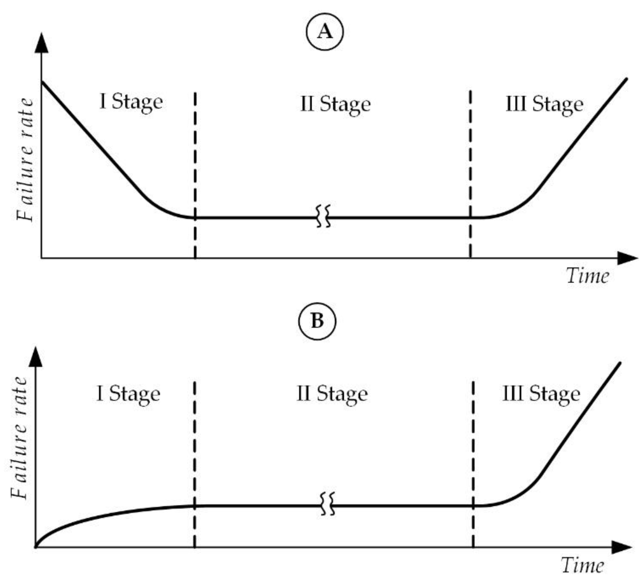
Figure 1. The failure rate in accordance with operation time; (A)—machines manufactured in individual production; (B)—machines manufactured in serial production.
Machines 10 00995 g001
Figure 2. The operational costs of engineering system.
Machines 10 00995 g002
Figure 3. Dependability of specific costs [EUR/wh] of a lifetime (Y-axis) and years (X-axis).
Machines 10 00995 g003
Figure 4. The function of cumulative maintenance costs f(t) and function of total costs of operating machine type 1.
Machines 10 00995 g004
Figure 5. The function of average costs for the machine type 1.
Machines 10 00995 g005
Figure 6. The first and second derivative of a function of average costs for the machine type 1.
Machines 10 00995 g006
Figure 7. The function of cumulative maintenance costs f(t) and function of total costs of operating machine type 2.
Machines 10 00995 g007
Figure 8. The function of average costs for the machine type 2.
Machines 10 00995 g008
Figure 9. The first and second derivative of a function of average costs for the machine type 2.
Machines 10 00995 g009
Table 1. Overview of failure rate and costs phenomenon in lifetime stages of different machine types.
Type of MachineStageFailure RateCosts
AI stage—Beginning of lifeDecreasing failure rateAdditional costs
BIncreasing failure rateMinimal costs
A & BII stage—Normal lifeThe low constant failure rateSlight increase in costs
III stage—End of lifeIncreasing failure rateStrong cost increase
Table 2. Specific costs of analyzed machines.
MachineType 1—CATType 2—LIE
YearOWC, [EUR/wh]OPC, [EUR/wh]HRC, [EUR/wh]TC, [EUR/wh]OWC, [EUR/wh]OPC, [EUR/wh]HRC, [EUR/wh]TC, [EUR/wh]
114.6226.7418.4357.7918.0418.0218.4354.49
226.4959.5423.0259.49
328.6061.6527.1863.65
437.0568.1026.9663.43
534.6467.6926.4762.94
632.9966.0432.0068.47
737.7870.8336.9173.38
826.8966.4236.3972.86
922.4467.4735.3071.77
1038.8578.3741.4077.87
Table 3. Calculated results of costs analysis.
MachineMinimal Costs LifetimeEconomic Lifetime
tC, YearsEUR/whtE, YearsEUR/wh
Type 13.5263.67.7070
Type 22.5560.16.8870
Publisher’s Note: MDPI stays neutral with regard to jurisdictional claims in published maps and institutional affiliations.