Article

Numerical Shape Planning Algorithm for Hyper-Redundant Robots Based on Discrete Bézier Curve Fitting

Department of Mechatronics and Machine Dynamics, Technical University of Cluj-Napoca, Str. Memorandumului, 28, 400114 Cluj-Napoca, Romania
*
Author to whom correspondence should be addressed.
Machines 2022, 10(10), 894; https://doi.org/10.3390/machines10100894
Submission received: 1 August 2022 / Revised: 23 September 2022 / Accepted: 28 September 2022 / Published: 3 October 2022

Abstract

:
The paper proposes a novel numerical method S-GUIDE that provides real-time planning of the shape of hyper-redundant robots with serial architecture by means of a guidance curve, represented in parametrized analytical form and in numerical form by a set of key points associated with the robot structure. To model the shape of the robot, the method uses an equivalent model, and a shape guidance curve obtained through a controlled adjustment of a Bézier curve. This is achieved in three computing steps were the robot equivalent structure, it’s associated kinematic parameters and the robot actuation parameters in joint space are calculated. The proposed method offers several advantages in relation with the precision, computing time and the feasibility for real-time applications. In the paper, the method accuracy, execution time, and the absolute error for different work scenarios are determined, compared and validated.

1. Introduction

Hyper-redundant robots (HRRs) are robotic mechanisms with a large or infinite degree of kinematic and/or actuator redundancy that have many similarities in shape and operation with snakes, tentacles, and elephants’ trunks as highlighted by Chirikjian et al. in [1,2]. Regarding their morphology, HRRs can be categorized as discrete and continuum/soft manipulators [3,4,5]. Discrete HRRs consists of a large and finite number of rigid links connected in series or a modular design approach where n identical modules (usually with 1-DoF, 2-DoF or 3-DoF topology [6]) are cascaded in series [7]. If the total number of degrees-of-freedom (DoF) tend to increase to infinity and the shape is continuously deformable we are discussing continuum/soft manipulators [8,9]. Both categories have their own advantages and disadvantages and area of applicability, and one category doesn’t exclude the other [4,5]. This paper addresses aspects related to discrete HRRs.
In the past few years, many discrete HRRs have been proposed as solutions for unstructured/dynamic environments where dexterous abilities and obstacle avoidance capabilities, to name a few, were important requirements to perform complex manipulation tasks [10]. Yeshmukhametov et al. [11] proposed TakoBot, a discrete hyper-redundant cable-driven continuum robot arm for harvesting cherry tomatoes with applicability in the agriculture industry. The robot is made up from 10 modules, each with 2-DoF (one module includes two discs interconnected through a universal joint) connected in series for a total of 20-DoF. The authors used an advanced motion planning algorithm based on video processing techniques to identify the cherry tomatoes and decide how to pick them. Their results indicates that the harvesting process can be improved by optimizing robot shape and trajectory. Canali et al. [12] developed SLIM, a cable-driven hyper-redundant robotic system for inspection and maintenance of infrastructures in industrial facilities. SLIM includes a 12-DoF robotic arm composed of 12 discrete modules, each one having one rotation (1 DoF). Their objective was to use a null-space approach to test if the robot can follow an imposed trajectory in the task space if path obstacles and limits of the actuators are considered. Based on experimental results they concluded that the imposed requirements can be fully accomplished if the accuracy of trajectory tracking is improved. Tang et al. [13] proposed a cable-driven hyper-redundant manipulator (CDHRM) for underwater applications. The robot was designed in such way that extra modules can be added or removed from the robot structure to offer greater flexibility in exploitation. The authors tested experimentally a prototype with five modules in an underwater environment for different trajectories and then compared their tracking results with other types of CDHRMs. Their proposed solution performed better due to the improved kinematic control algorithm. Besides these examples, there are many other applications and proposed solutions of HRRs in the medical field, aerospace industry, rescue scenarios and other unstructured environments. The reader should consult [14,15].
As can be seen in the literature, HRRs gained a lot of interests in the scientific world but their applicability is frequently limited to laboratory prototypes for different research activities. That’s because compared with traditional industrial robots, displacement analysis of HRRs is far more complex. Displacement analysis implies, among others, solving the robot’s forward kinematic problem (FKP) and inverse kinematic problem (IKP). FKP calculates the pose (position and orientation) of the end-effector when the inputs of the actuators are known while IKP calculates the required inputs of the actuators for a prescribed pose of the end-effector. FKP is used for example in robot shape and posture computation [7,16] or in simulations [17]. IKP is viewed as the foundation for trajectory planning and shape control algorithms [18]. Theoretically, due to the hyper redundancy nature of HRRs, IKP admits an infinite number of solutions [19]. This means that for a prescribed pose of the end-effector there are multiple shape correspondences (postures) of a HRR that satisfies the imposed constraints. Therefore, a shape planning strategy for designing motion control algorithms cannot be accomplished without a complex displacement analysis of HRRs.
As highlighted in [5,20], displacement analysis of HRRs can be solved with qualitative and quantitative models. Qualitative models are data-driven models based on learning algorithms that use input/output data sets. Popular approaches use fuzzy logic [21], genetic algorithms [22] and neural networks [23]. These types of models are very sensitive to datasets used for training and requires great computational resources. That is the reason why quantitative models became more popular in the literature. Quantitative models are classified as geometric and elasticity (mechanical) models. Both, geometric and elasticity models, are based on the concept of backbone curve (BC), a reference curve that models the macroscopic shape (spine) of the robot. The way the BC is modelled differentiates one approach from the other. In the case of geometric models, the piecewise constant curvature (PCC) approach proposed by Hannan [24] and the non-constant curvature approach (curve parametrization approach) proposed by Chirikjian [25] are widely used. On the other hand, elasticity models are usually based on Cosserat/Kirchhoff rod theories and captures, in addition to geometry of the BC, its elastic deformation by considering material properties of which it is made [26,27]. Whatever method is used, a choice must be made about the parametrization scheme of the BC for a particular task of the robot [28].
BC can be parametrized both intrinsically and extrinsically using parametric or non-parametric geometrical curves [5,20]. Non-parametric curves are not recommended for shape representation of HRRs due to their limitations [5]. Parametric curves can be expressed analytically—by using circles, ellipses, lines, helix, etc. or synthetically—by using Hermite curves, Bézier curves, B-Splines, non-uniform rational basis spline (NURBS), etc. [29,30]. Although analytical curves can be used to describe the shape of a HRR continuously from a starting point to a final point, they don’t have any intermediary control points to adjust the shape of the curve. Synthetic curves, on the other hand, are curves that are generated based on several control points and offers greater flexibility in controlling the shape of the BC [31]. Thus, many researchers proposed BC parametrization schemes using synthetic curves. Chirikjian [32] proposed a modal approach where the BC was modelled as a spline-like curve restricted to a set of intrinsic modes. However, the choice of the modes is not a simple task. Zanganeh et al. [33] parametrized extrinsically a reference BC by using 3rd and 5th order splines to solve the IKP of HRRs with different topologies. The approach was validated both for extensible and non-extensible variable geometry truss manipulators (VGTMs). The improved computational time using synthetic curves was highlighted also as an important advantage. Zhao et al. [18] proposed an inverse displacement analysis of a hyper-redundant elephant’s trunk robot (HRETR) by using a BC parametrized with modal functions. The HRETR robot consists of six discrete parallel mechanism modules connected in series. The idea was to generate a BC as a reference for the geometric characteristics of their robot and then to fit the modules of the robot on that curve. Once the shape of the robot was constructed, they could easily calculate IKP. One challenge was to find the corresponding shape of the robot configuration on the generated BC which depends on the robot kinematic configuration. Chibani et al. proposed in [19] a method for generating optimal reference kinematic configurations for HRRs based on BC parametrized with splines. Their method was tested on a real robot and lower computing times were also highlighted here as an advantage. Song et al. proposed in [34] a shape reconstruction algorithm for a wire-driven HRR based on a cubic Bézier curve and an electromagnetic sensor. The authors state that the Bézier curve is better than a spline curve to reconstruct the shape of HRRs if the position of the endpoints and vectors orientation at those points are known.
Even if the BC-based approaches, as highlighted above, were widely used with different methods as a way to solve the IKP of HRRs in the last decades, there are still important issues that need to be solved. An important aspect is related with the high computational time that these methods need [35], making them less suitable for real-time implementation. Another aspect is related with the positioning error due to the numerical algorithms used to implement the method and due to the fitting process of the robot modules on the curve [5,36]. Moreover, this error is in close dependence with the length of the robot, and it increases with the length of the robot. Parametrization of the BC is also an important issue. Synthetic curves are seen as being more advantageous in this matter due to their implicit way of construction using discrete data points.
In this context, the paper addresses the problem of determining the shape of HRRs with serial architecture by means of a guidance curve (BC), represented in parametrized analytical form and in numerical form by a set of key points associated with the robot structure. The main contribution of the paper is the proposed S-GUIDE method which uses a novel algorithm that fits an equivalent model on the parametrized guidance curve with high precision, the absolute error related to the method being of the order of microns. The accuracy does not depend on the length of the robot and can be indirectly controlled through a method input parameter. The execution time of the method allows its use in the development of real-time control algorithms of HRRs.
The S-GUIDE method can be used with different types of synthetic curves (spline, Bézier, Hermite etc.) to generate the BC. In this work the cubic Bézier curve was used due to the following advantages. The cubic Bézier curves are based on Bernstein polynomials (which have analytical solutions) and the solution of the curve is unique. A Bézier curve has endpoints common with a polygon and the tangents at the endpoints of the curve coincide with the first and last element of the polygon. This property allows defining the orientation and positioning of an end of the curve (robot end-effector in BC approach) by modifying two control points (last element of the polygon). If the geometry of a Bézier curve is modified, it never oscillates far from the control points (this allows to the curve-shifting algorithms to quickly find solutions in the immediate vicinity of a previous solution). Bézier curves can also be combined by joining their ends (common tangent) to form a composite curve whose geometry can be modified via control points. This property is exploited in the literature for dealing with the obstacle avoidance problem. A disadvantage of these type of curves is that the length of the curve is not in closed form, but it can be calculated using numerical methods.
The paper is structured as follows. Chapter 2 presents aspects regarding the conceptual description of the shape planning algorithm, while in Chapter 3 the performance of the proposed algorithm is evaluated, and the proposed S-GUIDE method is numerically tested for a virtual HRR (Python). The method accuracy, execution time, the absolute error for different work scenarios is determined, compared and validated. Finally, the paper ends with the conclusions.

2. Conceptual Description of Shape Planning Algorithm

For HRRs, the control of the shape during the handling operation (shape planning) is of distinct importance, especially in unstructured work environments. As previously seen, the shape of the robot can be simply described by a curve that follows the core of the robot, addressed in the literature as the backbone curve. The way of selecting this curve involves different approaches [2,37]. In this paper the BC is described (defined) by a set of key points Pi associated with the robot whose shape must be controlled. The Pi points are determined by constructing a simplified equivalent representation of the robot in the form of a virtual serial structure (see Figure 1), where the virtual joints are the Pi points. The simplified equivalent representation, with the choice of the Pi points, needs to be carried out so that the reconstruction of the robot is achievable starting from this representation.
In this context, assuming that (1) the modeling of the robot’s shape can be expressed through a parameterized curve on the entire robot’s working space, assuming that (2) a joint space solution exists for a shape described by such a curve, then the control of the shape of the robot in a manipulation task could be performed by controlling the parameters of this curve. In other words, under the specified assumptions the shape of the robot in the manipulation task can be controlled (guided) by means of a parametric curve, called the BC in the literature, used here as a shape guidance curve.
The first assumption involves that the shape of a HRR to be modeled by a spatial curve. If the robot’s backbone is described by a set of key points Pi associated with the centers of rotation of the robotic structure, then the problem is reduced to determining the curve passing through those points, the trivial solution leading to polynomial curves. So, the problem is not to find any curve that approximates the shape of the robot, but rather to identify a curve with a mathematical description as simple as possible that would allow modeling the shape of the robot described by the Pi points. The paper provides solutions in this sense using Bézier curves, curves with notable properties, for example these curves allow to define the orientation and position of the end-effector by only two parameters (two control points).
The second assumption (the existence of a solution in joint space) is conditioned by the robot’s architecture (kinematic configuration); therefore, any demonstration must be related to the specified targeted robot. In the current case, the research aimed a specific configuration (Python robot, a serially linked elements each defined by the length li), detailed in Chapter 3, which uses only universal joints to perform the motion. For a certain known architecture of a robot and a shape guidance curve, the problem of finding joint displacements which ensures the correspondence between robot and the imposed shape is called the shape inverse problem [38]. The solution existence for inverse shape problem is demonstrated and detailed in [38]. For a Python robot configuration, the existence of the solution for the inverse shape problem is conditioned only by the curvature value k of the shape guidance curve, which is limited by:
k 1 2 l m a x
where:
l m a x = max i ϵ { 1 , , n } l i
Under these specified assumptions the shape of the robot in the manipulation task can be controlled (guided) through a shape guidance curve (BC), by changing its parameters (the control points).
For solving the problem described above, a method is proposed (S-GUIDE) that uses numerical algorithms for iterative generation of the robot shape guide curve (BC) This allows it to run based on constraints related to the orientation and position imposed on the end-effector by path planning, which allows the transition from a shape space to a joint space (shape inverse problem, SIP [38]) and all of these in real-time operation. The proposed method is applied for HRRs which the equivalent model can be described through a serial topology with predefined lengths li for each element as presented in Figure 1.
The S-GUIDE method is structured on three steps which run sequentially. In the initial step the operating specifications (inputs) are updated at each sample time, in the third step the values of the joint’s displacements are provided which ensures robot folding on the imposed shape, thus completing the specified task through path planning. Table 1 briefly describes the specific steps of the proposed method. Their extensive description is detailed next.
Step 1—task specification: the algorithm inputs refer to the robot’s geometric characteristics, end-effector pose (position and orientation) and algorithm specific parameters (ex.: calculation precision of the robot BC). The robot’s geometric parameters (Figure 1) are: number of links n, length of the robot links l i   { i = 0 n } , position P 0 ( x 0 , y 0 , z 0 ) and orientation α 0 , β 0 , γ 0 of the fixed frame and the maxim angle between two adjacent elements θ m a x . The end-effector pose is defined through its position G ( x , y , z ) and orientation G α , G β , G γ . The algorithm parameters are: the maximum admitted error e b z for calculating the candidate Bézier curve and the maximum admitted error e r e in calculating the robot equivalent model.
The shape of the HRR through the associated Bézier curve (robot BC) is calculated between points P1 and Pn (Figure 1) which defines the position of the first and final joint in the structure. In addition, the position of these points P 1 ( x 1 , y 1 , z 1 ) and P n ( x n , y n , z n ) are calculated from the input data.
Step 2– robot shape planning: this step is composed of 2 algorithms, A1 −B-Curve candidate iterative generator and A2—Robot equivalent model reconstruction. (see Figure 2).
The algorithm A1- B-curve candidate iterative generation creates the Bézier candidate curve B(t) (Figure 3a) that is further used to define the robot BC (Figure 3b). For this, first the length reference for the Bézier candidate curve is calculated:
l t = i = 1 n l i
Next, the Bézier control points B 0 ,   B 1 ,   B 2 and B 3 are initialized. The position of B 0 and B 3 (starting and ending point of the B(t) curve) are associated with the points P1 and Pn of the robot that describe the position of the first and last joints in the kinematic chain. The other two points B 1 and B 2 , are placed on two support lines that pass through B0 and B1 and are colinear with the z axis of the O 0 x 0 y 0 z 0 and O n x n y n z n coordinate systems. By varying the position of B1 and B2 the length of the Bézier curve B(t) can be modified. The initial values for the two points are inherited from the solution found in the previous run of the S-GUIDE method. When the method is running for the first time, the position along the two-guidance lines for B 1 and B 2 are l t / 2 and l t / 2 , respectively.
The discretization of the Bézier curve is defined by the parameter Δ t . The value of this parameter is calculated using Equation (4).
Δ t e r e · 10 l t
The Bézier candidate curve is determined next in an iterative process by increasing/decreasing the distance between B 0 and B 1 , and B 3 and B 2 , respectively. At each iteration, the discretized Bézier curve B(t) is calculated using the equation:
B ( t ) = ( 1 t ) 3 B 0 + 3 ( 1 t ) 3 t B 1 + 3 ( 1 3 ) t 2 B 2 + t 3 B 3
where t = 0…1 with Δ t increment.
For this curve, the length is calculated and compared with the target value l t .
e 1 = l t j = 1 n b e z Δ x j 2 + Δ y j 2 + Δ y j 2
where: n b e z = 1 Δ t —number of discretized points on the Bézier curve.
Δ x j —cartesian distance along x axis between two consecutive points on B(t)
Δ y j —cartesian distance along y axis between two consecutive points on B(t)
Δ z j —cartesian distance along z axis between two consecutive points on B(t)
If the absolute value of the error | e 1 | (Equation (6)) is greater than e b z , new positions for the B 1 and B 2 are calculated. The new positions results from adding to the current position of B 1 and B 2 along the support lines by the value e 1 / 3 . If | e 1 | is smaller or equal to e b z the iteration stops, and the obtained B(t) curve is considered the candidate Bézier curve.
The positions for the control points B 1 and B 2 are memorized and used as a starting point to calculate the first Bézier candidate curve in the next S-GUIDE cycle, for the next position and orientation of the end-effector defined by its trajectory.
The algorithm A2-Robot equivalent model reconstruction uses the candidate Bézier curve B(t) to further refine it in order to be able to reconstruct an equivalent robot model (ERM) on the backbone curve BR(t) (Figure 3b). The ERM is further used, in S-GUIDE step 3, to calculate the SIP.
The backbone curve BR(t) is iteratively obtained by adjusting the candidate Bézier curve B(t). At each step in the iteration the ERM is reconstructed from P1 to Pi−1. The length dn−1 of the final element in the model is obtained by calculating the distance between the points Pi−1” (point belonging to the equivalent robot model) and point Pn calculated in step 1 from the position of end-effector. The obtained distance dn−1 is compared with the length of the n−1 element l n 1 , resulting in the error e 2 (Equation (7)).
e 2 = d n 1 l n 1
If the error | e 2 | is greater than the imposed e r e new positions for the points B 1 and B 2 are calculated. The new position is obtained by adding to the current positions of the two points along the support lines the value e 2 / 3 and e 2 / 3 , respectively. After this adjustment the backbone curve BR(t) is recalculated, and the iterative process on A2 starts from the beginning. The iteration loop ends when the condition | e 2 | < e r e is fulfilled.
The reconstruction process of the ERM in the above iteration is accomplished by sequentially adding elements in model (Figure 3b) at each level the sequence:
-
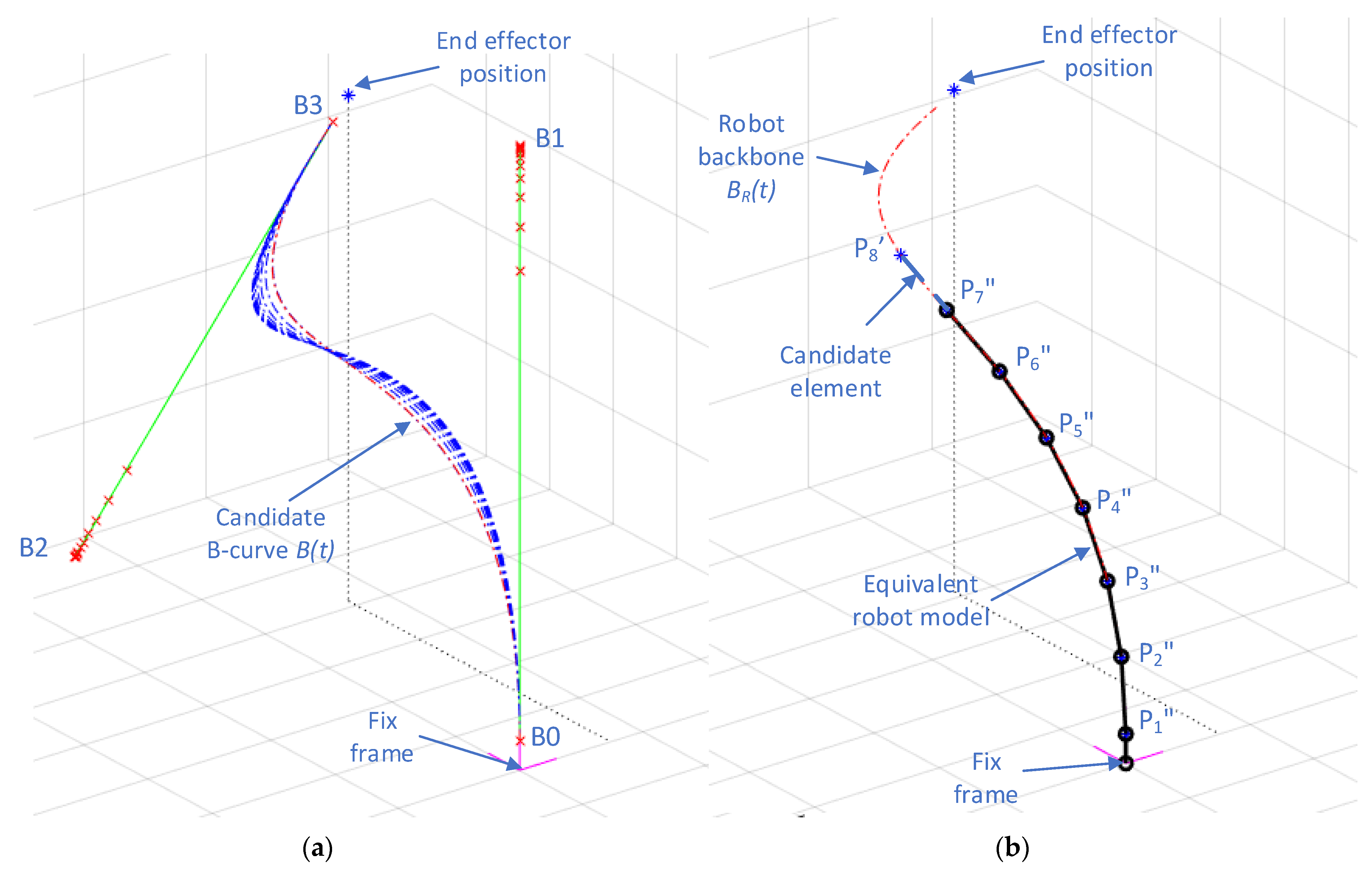
The position of point Pj′ {j = 2…n−1} belonging to the backbone curve BR(t) is determine by finding a segment (candidate element) on the BR(t) curve that has the length ≈ lj−1. The length of the candidate element is measured between the point Pi ϵ BR(t) and the point Pj−1 ϵ ERM that defines the end of the previous element.
-
For each obtained Pj′ the spherical coordinates are measured in respect to a coordinate system placed in Pj−1″ that has the orientation of the global coordinate system.
a z j = a r c t a n 2 ( P x j P x j 1 , P z j P z j 1 ) e l j = a r c t a n 2 ( P z j P z j 1 , P y j P y j 1 )
-
Using the angles a z j and e l j and the length lj, the elements j−1 from the ERM is constructed by finding the position of point P j ϵ ERM using Equation (9).
P x j = P x j 1 + l j cos ( e l j ) cos ( a z j ) P y j = P y j 1 + l j cos ( e l j ) sin ( a z j ) P z j = P z j 1 + l j sin ( e l j )
After finalizing A2, the output is the robot’s ERM (defined by a set of points P i   { i = 1 n } and their spherical coordinates).
Step 3 – shape inverse problem: in the third step the obtained ERM is validated and the kinematic parameters for the inverse shape problem are calculated.
For validating the ERM model, the angle θ i   { i = 1 n } between every two consecutive elements in the model are calculated (Equation (12)). The two elements are described as vectors (Equations (10) and (11)) and the angle calculation is reduced to find the angle between the two.
v i 1 ¯ = [ P x i P x i 1 , P y i P y i 1 , P z i P z i 1   ]
v i ¯ = [ P x i + 1 P x i , P y i + 1 P y i , P z i + 1 P z i   ]
θ i = a t a n 2 ( | | v i 1 x   v i | | , v i 1 · v i )
All values of θ i are verified to be less than θ m a x . If the condition is not fulfilled the input data (robot configuration and the end-effector pose) fails to have a solution that could be described by the method.
Next the rotation matrix for each element in the ERM is calculated. For this, first the absolute angles for each element along the x and y axis is calculated using Equation (13).
α i = asin ( d x i d y i 2 + d z i 2 ) β i = atan 2 ( d x i , d z i )
where: d x i = P x i P x i 1
d y i = P y i P y i 1
d z i = P z i P z i 1
The R i 0 rotation matrix is obtained using:
R i 0 = [ c o s β i 0 s i n β i 0 1 0 s i n β i 0 c o s β i ] [ 1 0 0 0 c o s α i s i n α i 0 s i n α i c o s α i ]
For calculating the actuation angles θ x i and θ y i in each of the universal joint, each point Pi from the ERM model is represented in a local coordinate system attached to the i−1 element, that have the z axis colinear with the element. These values are obtained by multiplying the inverse rotation matrix R i 1 0 with the position vector of point Pi.
[   P i 1 x i P i 1 y i P i 1 z i ] = i n v ( R i 1 0 ) [ P x i P y i P z i ]
These positions (Equation (15)) are used to calculate the θ x i and θ y i   { i = 1 n } relative angles using:
θ x i = asin ( P i 1 x i P i 1 y i 2 + P i 1 z i 2 ) θ y i = atan 2 ( P i 1 x i , P i 1 z i )
For the Python robot, its shape is defined by the angles θ x i , θ y i .

3. Numerical Results

The experimental results were developed using the MATLAB/Simulink environment developed by MathWorks. These experiments aimed to assess the performance of the method and to validate the results by planning the shape of the robot Python for a given manipulation task.

3.1. Performance Assessment of the S-GUIDE Method

In this section, the S-GUIDE method precision is evaluated, and the time needed for one processing cycle (Figure 4) is determined.
First, the method was tested for calculating the backbone shape of a robot structure that is composed from n = 12 element that have identical length li. Two experiments were developed that imposed a 3D trajectory for the end-effector through a spline curve defined by four points in the robot’s workspace.
The spline curve which defines the end effector trajectory was discretized in m = 26 sections/points that represent the reference for the end-effector (G point position and orientation). In the first case the orientation of the end-effector was constant ( G α = 110   [ d e g ] ,   G β = 0   [ d e g ] ,   G γ = 0   [ d e g ] ), and in the second case the orientation of the end-effector varied ( G α = 110 20   [ d e g ] ,   G β = 0   [ d e g ] ,   G γ = 0   [ d e g ] ). The obtained back bone curves for the two experiments are presented in Figure 5.
For each obtained BC (posture), the absolute position errors e G i { i = 1 m } for the end-effector were calculated. The e G i error is directly connected to the values of e r e and Δ t . The BCs presented in Figure 5 are calculated using e r e = 0.001   [ m m ] and Δ t is calculated using Equation (4) ( Δ t = 0.0001 ).
In order to evaluate the influence of parameter Δ t in relation with e G i , two other values were used for Δ t . The values used for Δ t were: 0.0005 (does not fulfil Equation (4)) and 0.00005 (fulfil Equation (4)). The obtained variations of the absolute position errors e G i for the two experiments with constant and variable end-effector orientations are presented in Figure 6.
It was observed that for the situation where the parameter Δ t did not fulfil the condition in Equation (4) there were spikes in the absolute errors due to the impossibility to find a final solution that respects the imposed e r e parameter for the ERM. For the situation where Δ t fulfiled the condition in Equation (4) the mean absolute errors (MAE) for e G i are presented in Table 2.
Decreasing or increasing the value of the parameters e r e (directly influencing the Δ t parameter through Equation (4)) influenced the computational time. As a result, depending on the application and the hardware resources for the control system the precision of the algorithm could be adjusted to best suit each situation. The average time needed for computing each step in the method for different e r e values for a robot structure with 12 modules (24 DoF) is presented in Table 3. The experiments were developed in MATLAB using a Lenovo working station with an i7−10750H processor at 2.6 GHz running Windows 10 OS developed by Microsoft.
It was observed (Table 3) that the time needed to compute steps 3.1 and 3.2 was not influenced by the variation of the e r e . Step 3 (3.1 and 3.2) calculation time was directly connected with the robot topological configuration. The A1 and A2 computational times was influenced by the variation of e r e . Decreasing the e r e directly decreased parameter Δ t , that influenced the discretization step of the candidate Bézier curve and the process of calculating the robot backbone and ERM reconstruction.
The cycle time was further evaluated for four HRR robots that had 18, 24, 30 and 36 DoF that had elements with same length l i = c t . The obtained average times for a cycle after completing the trajectory (discretized in 26 points) are presented in Table 4.
In Figure 7 the obtained cycle times for e r e that vary from 0.1 mm to 0.0005 mm are presented. As can be observed, for e r e errors that were equal or higher than 0.05 mm the total cycle processing time was less than 2.1 ms for all four HRRs. These values make the S-GUIDE method suitable for real-time application implementation.

3.2. S-GUIDE Method Testing for the Python Robot

For validating the S-GUIDE method, the IKP for a 24-DoF hyper-redundant robot Python was calculated for a given task. The robot structure consisted of n = 12 identical modules that were serially connected through universal joints (Figure 8). Each module had 2 DoF allowing two relative rotations between the upper and lower platform of each module along the Oix and Oiy {i = 112} local coordinate axis [7]. The actuation of each module was accomplish using two pairs of bellows that work in tandem in order to impose the rotation angles in the universal joints (Figure 8a).
The robot is intended to be used in farming activities that are related to fruit/vegetable harvesting. For this reason, the last module integrated a soft gripper produced by SoftGripping Co. [10]. In relation to the aforementioned activities, the robot’s tasks are:
-
remain in a home position until a harvest command is received
-
determine the needed trajectory from the home position to the object to grasp
-
perform grasping
-
place the object in designated containers and return to the home position.
In the developed experiment, the S-GUIDE method was used to calculate the robot’s shape for a task of grasping an object placed in the robot’s workspace. The robot started from the home position and using an already determined trajectory the robot’s inverse shape was calculated for the whole process.
In order to simulate the process, a model of the robot was implemented in MATLAB/Simulink using Simscape components. Simscape allows the attachment of sensors in the robot’s structure that can be used to measure the kinematic parameters of the robot. The input for the robot model are the angles for the universal joints. During simulations the ideal representation of the robot is used, which does not take into consideration any potential joint manufacturing errors, deflection of joints due to mechanical loads or the control system performance. Using this representation, it allowed the evaluation of the S-GUIDE method’s algorithm errors obtained due to deviation from the imposed trajectory.
In the developed experiment, a grasping task was simulated. The robot started to move from the home position at Gx = 0 mm Gy = 390 mm and Gz = 435 mm with the orientation Gα = −110 deg, Gβ = 0 deg and Gγ = 0 deg (Figure 9b). From this position the end-effector moved to Gx = 0 mm, Gy = 578 mm and Gz = 345 with the final orientation Gα = −90 deg, Gβ = 0 deg, and Gγ = 0 deg (Figure 9c). The transition between the start and stop points was implemented using a spline with three intermediary points, the orientation Gα was changed linearly between the initial value to the final value.
The parameters used as input data for the S-GUIDE method were: the number of modules n = 12 , length of each element l i   { i = 0 12 } resulting in the total length of the robot being 799 mm, and a maximum angle between two adjacent elements θ m a x = 30   d e g . The initial position of the end-effector, and the position and orientation of the base was as mentioned above. The parameters e b z and e r e are 0.5 mm and 0.05 mm.
The obtained backbone curves for the robot along the imposed trajectory are displayed in Figure 9a.
For each robot pose during the trajectory transition of the end-effector, the S-GUIDE method provides the joint angles θ x i and θ y i  {i = 112} for all robot modules. The variation of the joint angles during the simulation is presented in Figure 10. The obtained values vary smoothly during the simulation.
The variation of the imposed position for P12 (reference value) and the position resulting at the robot’s 12th universal joint (the associated point P12 on the robot) are presented in Figure 11a. The obtained absolute errors between the two parameters along the Ox, Oy and Oz axis are displayed in Figure 11b.
The obtained MAE errors during the simulation were: 0 mm for Px12 position, 0.051 mm for Py12 position and 0.0151 mm for Pz12 position. These values were in the same range as the imposed ere, and were characterized by slight random fluctuation around ere.
The imposed trajectory (blue) and the simulation results (red) for the end-effector positions are presented in Figure 12a. The end-effector position error e T is presented in Figure 12b. The obtained MAE, 0.0537 mm and 0.006%, represents the method error (S-GUIDE algorithm) for a preset input parameters ( e b z = 0.5 mm e r e = 0.05 mm) and for an ideal robot (without joint errors, structure bending and torsion etc.).

3.3. Discussions and Results Comparison

The developed experiments aimed to test the S-GUIDE method from three perspectives: precision, computational time and quality of the obtained solution. The precision of the results for the method is directly connected with the algorithm parameter e r e . During the developed experiments the imposed values for the e r e parameter varied from 0.0005 mm to 0.5 mm. It was observed that varying this value directly influenced the computational time of the method. For the developed experiments where the structures with DoFs varying from 18 to 36, a good tradeoff for e r e was the value 0.05 mm (the length of the robots varied from 605 mm to 1211 mm) at which the computational time for all tested robots was less than 2.1 ms. If the value for the e r e parameter was increased the computational time decreased (e.g., for an e r e = 0.5 for an 18-DoF structure the computational time was 0.846 ms). The experimental results emphasize that the robot joints have incremental and uniform movements that ensured a fluid motion of the structure along the imposed trajectories.
In the proposed algorithm, another advantage is the fact that the precision of the solution remains in the same range for a given value of the e r e parameter and does not depend on the robot’s number of modules or length.
To evaluate the performance of the proposed S-GUIDE method, the obtained results were compared with the results presented in the literature that used other techniques to calculate the robot’s shape and IKP. The comparation took in account the execution time and the end-effector position error:
-
a comparative study between different algorithms for solving the IKP problem for a 10-DoF structure was presented in [36]. The authors used an exhaustive method and error optimization algorithms for this purpose. It was observed that the exhaustive methods gave good results on positioning errors, but the processing time was fairly high and not applicable for real-time applications (ex.:18 s for a 4 DoF structure). Using error optimization algorithms (Patternsearch, Genetic algorithms, Multistart and Simulannelbnd), the computation time for a 10-DoF robot varied from 0.5 s to 14 s with errors that ranged from 4 to 10 mm. Using S-GUIDE for a 24-DoF robot, the computational time was 0.001 s with an average positioning error of 0.0537 mm.
-
Another method proposed for calculating the inverse kinematics of HRRs called PASO is based on a particle swarm optimization algorithm and was presented in [35]. Using this method for a 30-DoF robot (ReMod3D) a processing time of 1.57 s with an average positioning error of 0.46 mm was obtained. Using S-GUIDE for a robot with 30 DoF the processing time was 0.001731 s with a similar positioning precision.
-
A good performance in relation to the computational time was obtained using the natural CCD algorithm presented in [39]. For a 20-DoF robot (integrates joints with 2 DoF) the processing time was around 0.05 s with a precision of 0.1. Using S-GUIDE for a 24-DoF robot the computational time was 0.001 s with a precision of 0.006%.
From the above comparisons, the proposed method offers good execution time and positioning errors in relation to state-of-the-art algorithms. The obtained precision and low computational time make this method a good candidate for integration into control algorithms for these type of robots.
There are also some method limitations: the proposed algorithm’s search BC solutions for a given orientation for the robot base does not modify the orientation of the base in order to calculate a wider range of solutions when the joint angle limit is reached. The S-GUIDE method calculates the HRR’s IKP solution using a cubic Bézier curve, further developments which combine multiple cubic Bézier curves aim to increase the robustness of the path planning and include functionalities for obstacle avoidance.

4. Conclusions

The proposed S-GUIDE method allows the planning the shape of HRRs with serial architecture, obtaining and driving the shape of this class of robots in real-time manipulation processes. To model the shape of the robot, the method uses an equivalent model, a shape guidance curve (BC) obtained through a controlled adjustment of a Bézier curve. The method is characterized by high precision (of the order of microns) which is maintained regardless of the length of the robot. For a HRR composed of 12 modules (Python), the following results were obtained: the processing time related to one cycle is less than 2 ms, with a precision of 0.0537 mm.
In addition, the precision can be adjusted through the e r e input parameter, which gives an important advantage in real-time applications (e g., for a method error of 0.05 mm, for all tested HRRs (18 DoF-36 DoF) configurations, the execution time is below 2 ms, if the imposed error increases, the execution times related to the method decrease).
The proposed method can also be extended to HRRs with other topologies which can be functionally reduced to the equivalent model the method works with.

Author Contributions

Conceptualization, C.L. and O.H.; methodology, C.L., O.H. and C.R.; software, C.L.; validation, C.L., O.H. and C.R.; formal analysis, C.L., O.H. and C.R.; investigation, C.R., O.H. and C.L.; resources, C.L., O.H. and C.R.; data curation, C.L.; writing—original draft preparation, C.L., C.R. and O.H.; writing—review and editing, C.L., C.R. and O.H.; visualization, C.L.; supervision, O.H.; project administration, O.H.; funding acquisition, O.H. All authors have read and agreed to the published version of the manuscript.

Funding

This research was funded by the Romanian Ministry of Education and Research, CCCDI—UEFISCDI, project number PN-III-P2-2.1-PED-2019-4939, within PNCDI III https://uefiscdi.gov.ro/proiect-experimental-demonstrativ-ped (accessed on 21 July 2022).

Acknowledgments

This work was supported by a grant from the Romanian Ministry of Education and Research, CCCDI—UEFISCDI, project number PN-III-P2-2.1-PED-2019-4939, within PNCDI III”.

Conflicts of Interest

The authors declare no conflict of interest. The funders had no role in the design of the study; in the collection, analyses, or interpretation of data; in the writing of the manuscript, or in the decision to publish the results.

References

  1. Chirikjian, G.S.; Joel, W.B. An obstacle avoidance algorithm for hyper-redundant manipulators. In Proceedings of the IEEE International Conference on Robotics and Automation, Cincinnati, OH, USA, 13–18 May 1990; pp. 625–631. [Google Scholar] [CrossRef] [Green Version]
  2. Chirikjian, G.S. Theory and Applications of Hyperredundant Robotic Mechanisms. Ph.D. Thesis, Department of Applied Mechanics, California Institute of Technology, Pasadena, CA, USA, 22 May 1992. Available online: https://thesis.library.caltech.edu/4458/1/Chirikjian_gs_1992.pdf (accessed on 21 July 2022).
  3. Rad, C.; Hancu, O.; Lapusan, C. Aspects regarding “soft” grasping in smart agricultural harvesting tasks. Acta Tech. Napoc. Ser. Appl. Math. Mech. Eng. 2020, 63, 389–394. [Google Scholar]
  4. Martín-Barrio, A. Design, Modelling, Control and Teleoperation of Hyper-Redundant Robots. Ph.D. Thesis, Universidad Politécnica de Madrid, Madrid, Spain, 2 November 2020. Available online: https://oa.upm.es/65161/1/ANDRES_MARTIN_BARRIO.pdf (accessed on 21 July 2022).
  5. Singh, I. Curve Based Approach for Shape Reconstruction of Continuum Manipulators. Ph.D. Thesis, Universite de Lille, Lille, France, 2018. Available online: https://hal.archives-ouvertes.fr/tel-01967054/document (accessed on 21 July 2022).
  6. Liu, J.; Tong, Y.; Liu, J. Review of snake robots in constrained environments. Robot. Auton. Syst. 2021, 101, 103785. [Google Scholar] [CrossRef]
  7. Lapusan, C.; Hancu, O.; Rad, C. Shape Sensing of Hyper-Redundant Robots Using an AHRS IMU Sensor Network. Sensors 2022, 22, 373. [Google Scholar] [CrossRef] [PubMed]
  8. Walker, I.D. Continuous backbone “continuum” robot manipulators. ISRN Robot. 2013, 2013, 726506. [Google Scholar] [CrossRef] [Green Version]
  9. Kolachalama, S.; Lakshmanan, S. Continuum robots for manipulation applications: A survey. J. Robot. 2020, 2020, 4187048. [Google Scholar] [CrossRef]
  10. Rad, C.; Hancu, O.; Lapusan, C. Data-Driven Kinematic Model of PneuNets Bending Actuators for Soft Grasping Tasks. Actuators 2022, 11, 58. [Google Scholar] [CrossRef]
  11. Yeshmukhametov, A.; Koganezawa, K.; Yamamoto, Y.; Buribayev, Z.; Mukhtar, Z.; Amirgaliyev, Y. Development of Continuum Robot Arm and Gripper for Harvesting Cherry Tomatoes. Appl. Sci. 2022, 12, 6922. [Google Scholar] [CrossRef]
  12. Canali, C.; Pistone, A.; Ludovico, D.; Guardiani, P.; Gagliardi, R.; De Mari Casareto Dal Verme, L.; Sofia, G.; Caldwell, D.G. Design of a Novel Long-Reach Cable-Driven Hyper-Redundant Snake-like Manipulator for Inspection and Maintenance. Appl. Sci. 2022, 12, 3348. [Google Scholar] [CrossRef]
  13. Tang, J.; Zhang, Y.; Huang, F.; Li, J.; Chen, Z.; Song, W.; Zhu, S.; Gu, J. Design and Kinematic Control of the Cable-Driven Hyper-Redundant Manipulator for Potential Underwater Applications. Appl. Sci. 2019, 9, 1142. [Google Scholar] [CrossRef] [Green Version]
  14. Lapusan, C.; Rad, C.; Hancu, O. Kinematic analysis of a hyper-redundant robot with application in vertical farming. IOP Conf. Ser. Mater. Sci. Eng. 2021, 1190, 012014. [Google Scholar] [CrossRef]
  15. Martin, A.; Terrile, S.; Barrientos, A.; del Cerro, J. Hyper-redundant robots: Classification, state-of-the-art and issues. Rev. Iberoam. De Automática E Inf. Ind. 2018, 15, 351–362. [Google Scholar] [CrossRef]
  16. Lee, C.; An, D. AI-Based Posture Control Algorithm for a 7-DOF Robot Manipulator. Machines 2022, 10, 651. [Google Scholar] [CrossRef]
  17. Lapusan, C.; Hancu, O.; Rad, C. Quaternion-Based Approach for Solving the Direct Kinematics of a Modular Hyper Redundant Robot. Acta Tech. Napoc. Ser. Appl. Math. Mech. Eng. 2020, 63, 363–366. [Google Scholar]
  18. Zhao, Y.; Jin, L.; Zhang, P.; Li, J. Inverse Displacement Analysis of a Hyper-redundant Elephant’s Trunk Robot. J. Bionic Eng. 2018, 15, 397–407. [Google Scholar] [CrossRef]
  19. Chibani, A.; Mahfoudi, C.; Chettibi, T.; Merzouk, R.; Zaatri, A. Generating optimal reference kinematic configurations for hyper-redundant parallel robots. Proc. Inst. Mech. Eng. Part I J. Syst. Control Eng. 2015, 229, 867–882. [Google Scholar] [CrossRef]
  20. Bieze, T.M. Contribution to the Kinematic Modeling and Control of Soft Manipulators Using Computational Mechanics. Ph.D. Thesis, Universite de Lille, Lille, France, 24 October 2017. Available online: https://hal.archives-ouvertes.fr/tel-03516545/document (accessed on 21 July 2022).
  21. Qi, P.; Liu, C.; Zhang, L.; Wang, S.; Lam, H.-K.; Althoefer, K. Fuzzy logic control of a continuum manipulator for surgical applications. In Proceedings of the IEEE International Conference on Robotics and Biomimetics (ROBIO), Bali, Indonesia, 5–10 December 2014; pp. 413–418. [Google Scholar] [CrossRef]
  22. Runge, G.; Peters, J.; Raatz, A. Design optimization of soft pneumatic actuators using genetic algorithms. In Proceedings of the IEEE International Conference on Robotics and Biomimetics (ROBIO), Macau, Macao, 26 March 2018; pp. 393–400. [Google Scholar] [CrossRef]
  23. Melingui, A.; Lakhal, O.; Daachi, B.; Mbede, J.B.; Merzouki, R. Adaptive Neural Network Control of a Compact Bionic Handling Arm. IEEE/ASME Trans. Mechatron. 2015, 20, 2862–2875. [Google Scholar] [CrossRef]
  24. Hannan, M.W.; Walker, I.D. Novel kinematics for continuum robots. In Advances in Robot Kinematics; Lenarčič, J., Stanišić, M.M., Eds.; Springer: Dordrecht, Netherlands, 2000; pp. 227–238. [Google Scholar]
  25. Chirikjian, G.S. Conformational Modeling of Continuum Structures in Robotics and Structural Biology: A Review. Adv. Robot. 2015, 29, 817–829. [Google Scholar] [CrossRef] [PubMed] [Green Version]
  26. Trivedi, D.; Lotfi, A.; Rahn, C.D. Geometrically Exact Models for Soft Robotic Manipulators. IEEE Trans. Robot. 2008, 24, 773–780. [Google Scholar] [CrossRef]
  27. Trivedi, D.; Rahn, C.D.; Kier, W.M.; Walker, I.D. Soft robotics: Biological inspiration, state of the art, and future research. Appl. Bionics Biomech. 2008, 5, 99–117. [Google Scholar] [CrossRef]
  28. Wang, T.; Lin, B.; Chong, B.; Whitman, J.; Travers, M.; Goldman, D.I.; Blekherman, G.; Choset, H. Reconstruction of backbone curves for snake robots. IEEE Robot. Autom. Lett. 2021, 6, 3264–3270. [Google Scholar] [CrossRef]
  29. Zeid, I. Mastering CAD/CAM, 1st ed.; McGraw-Hill Science/Engineering/Math: New York, NY, USA, 2004. [Google Scholar]
  30. Sarcar, M.M. Computer Aided Design and Manufacturing, 1st ed.; Prentice-Hall of India Pvt. Ltd: Delhi, India, 2008. [Google Scholar]
  31. Pérez, L.H.; Aguilar, M.C.M.; Montés Sánchez, N.; Montesinos, A.F. Path Planning Based on Parametric Curves. In Advanced Path Planning for Mobile Entities; Róka, R., Ed.; IntechOpen: London, UK, 2017; pp. 125–143. [Google Scholar]
  32. Chirikjian, G.S.; Burdick, J.W. A modal approach to hyper-redundant manipulator kinematics. IEEE Trans. Robot. Autom. 1994, 10, 343–354. [Google Scholar] [CrossRef] [Green Version]
  33. Zanganeh, K.E.; Angeles, J. The inverse kinematics of hyper-redundant manipulators using splines. In Proceedings of the IEEE International Conference on Robotics and Automation, Nagoya, Japan, 21–27 May 1995; pp. 2797–2802. [Google Scholar] [CrossRef]
  34. Song, S.; Li, Z.; Yu, H.; Ren, H. Shape reconstruction for wire-driven flexible robots based on Bézier curve and electromagnetic positioning. Mechatronics 2015, 29, 28–35. [Google Scholar] [CrossRef]
  35. Collins, T.; Shen, W.M. PASO: An Integrated, Scalable PSO-Based Optimization Framework for Hyper-Redundant Manipulator Path Planning and Inverse Kinematics; Technical Report No. ISI-TR-697; Information Sciences Institute, University of Southern California (USC) Viterbi School of Engineering: Los Angeles, CA, USA, 2016. [Google Scholar]
  36. Espinoza, M.S.; Gonçalves, J.; Leitao, P.; Sánchez, J.L.G.; Herreros, A. Inverse kinematics of a 10 DoF modular hyper-redundant robot resorting to exhaustive and error-optimization methods: A comparative study. In Proceedings of the 2012 Brazilian Robotics Symposium and Latin American Robotics Symposium, Fortaleza, Brazil, 16–19 October 2012; pp. 125–130. [Google Scholar] [CrossRef] [Green Version]
  37. Gravagne, I.A.; Walker, I.D. Manipulability, force, and compliance analysis for planar continuum manipulators. IEEE Trans. Robot. Autom. 2002, 18, 263–273. [Google Scholar] [CrossRef] [PubMed] [Green Version]
  38. Mochiyama, H.; Shimemura, E.; Kobayashi, H. Shape correspondence between a spatial curve and a manipulator with hyper degrees of freedom, In Proceedings of the IEEE/RSJ International Conference on Intelligent Robots and Systems. Innovations in Theory, Practice and Applications, Victoria, BC, Canada, 17 October 1998; Volume 1, pp. 161–166. [Google Scholar] [CrossRef]
  39. Martin, A.; Barrientos, A.; Del Cerro, J. The natural-CCD algorithm, a novel method to solve the inverse kinematics of hyper-redundant and soft robots. Soft Robot. 2018, 5, 242–257. [Google Scholar] [CrossRef] [PubMed]
Figure 1. Kinematic diagram—equivalent robot model.
Machines 10 00894 g001
Figure 2. S-GUIDE method steps (a) Task specification initial points (b) Attached robot shape on the Bézier curve (c) Robot shape based on the algorithm results.
Machines 10 00894 g002
Figure 3. Robot shape planning (a) calculating the candidate Bézier curve (algorithm A1) (b) reconstruction of the equivalent robot model (algorithm A2).
Machines 10 00894 g003
Figure 4. Step processing cycle.
Machines 10 00894 g004
Figure 5. Calculation of the BC for a 3D imposed trajectory (a) constant orientation for the end-effector (b) variable orientation for the end-effector.
Machines 10 00894 g005
Figure 6. Variation of the absolute positioning error e G i (a) for constant orientation of the end−effector (b) for variable orientation of the end−effector.
Machines 10 00894 g006
Figure 7. Cycle time variation for different e r e values.
Machines 10 00894 g007
Figure 8. Python robot (a) detailed view of a module (b) CAD model.
Machines 10 00894 g008
Figure 9. Python virtual model in Simscape (a) backbone curve for the imposed trajectory (b) initial position (c) final position.
Machines 10 00894 g009
Figure 10. Variation of the joint angles (a) angle θ x i (b) angle θ y i .
Machines 10 00894 g010
Figure 11. Simulation results (a) variation of the end-effector position along the Ox, Oy and Oz axis (b) variation of the absolute error.
Machines 10 00894 g011
Figure 12. Simulation results (a) end-effector trajectory (b) position error.
Machines 10 00894 g012
Table 1. S-GUIDE method. Short description and symbolic graphical representation of each method steps.
I. Task SpecificationsII. Robot Shape PlanningIII. Shape Inverse Problem
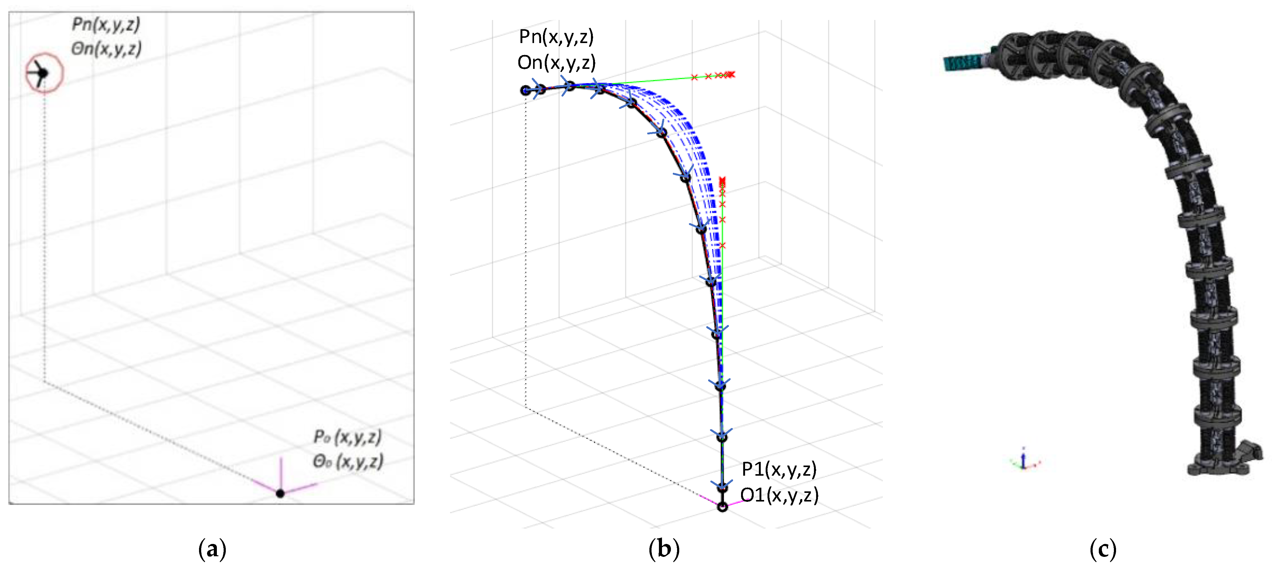
Specifying the robot’s geometric characteristics, end-effector pose (position and orientation) and algorithm specific parameters. (See Figure 2a)Based on the operational specifications, a candidate 3D Bézier parametric curve for modeling the shape of the robot is generated (A1). Further, the candidate curve is iteratively adjusted (BC of HRR) simultaneously with the reconstruction of an equivalent model of the robot (A2). (See Figure 2b)For a particular robotic structure (here, a Python robot) and a planned 3D shape the joint displacements are determined (based on step 3 results). (See Figure 2c)
Table 2. Variation of MAE.
Experiment MAE   ( Δ t = 0.0001 )
(mm)
MAE   ( Δ t = 0.00005 )
(mm)
Constant orientation for end −effector0.00120.00077
Variable orientation for end −effector0.00190.00076
Table 3. Cycle time for different imposed values for e r e .
Method   Imposed   Error   e r e
(mm)
Step 2 A1 Time
(s)
Step 2 A2
Time
(s)
Step 3.1 Time
(s)
Step 3.2 Time
(s)
Cycle Time
(s)
e r e = 0.5 0.0003840.0003180.0000540.0001030.000859
e r e = 0.1 0.0004030.0003340.0000550.0001050.000897
e r e = 0.05 0.0003910.0005070.0000550.0001060.001059
e r e = 0.01 0.0004410.00130.0000600.0001080.001909
e r e = 0.005 0.0004900.00220.0000620.0001060.002858
e r e = 0.001 0.00110.01140.0000610.0001030.012664
e r e = 0.0005 0.00220.02510.0000620.0001070.027469
Table 4. Cycle time for robots with different DoFs and imposed values for e r e
Method   Imposed   Error   e r e
(mm)
Cycle Time for HRR 18 DoF
(s)
Cycle Time for HRR 24 DoF
(s)
Cycle Time for HRR 30 DoF
(s)
Cycle Time for HRR 36 DoF
(s)
e r e = 0.5 0.0008460.0008590.0014140.001414
e r e = 0.1 0.0008670.0008970.0016490.001726
e r e = 0.05 0.0010370.0010590.0017310.002053
e r e = 0.01 0.0016650.0019090.0042470.004725
e r e = 0.005 0.0027140.0028580.0069680.008511
e r e = 0.001 0.010120.0126640.033280.041637
e r e = 0.0005 0.022740.0274690.0644860.064486
Publisher’s Note: MDPI stays neutral with regard to jurisdictional claims in published maps and institutional affiliations.

