Application of Improved Robust Local Mean Decomposition and Multiple Disturbance Multi-Verse Optimizer-Based MCKD in the Diagnosis of Multiple Rolling Element Bearing Faults

Abstract

Rolling element bearings are an important joint in mechanical equipment and have a high engineering application value. To solve the problem of the difficulty in extracting periodic fault pulses due to complex noise interference and the interference of transmission paths in rolling element bearing fault characteristic signals, a novel hybrid fault diagnosis method based on complementary complete ensemble robust local mean decomposition with adaptive noise (CCERLMDAN) combined with multiple disturbance multi-verse optimizer (MDMVO)-based Maximum correlated Kurtosis deconvolution (MCKD) is proposed in this paper, and applied in different rolling element bearing fault conditions. Firstly, the CCERLMDAN method adaptively decomposes the fault vibration signal into multiple product functions (PF), and then selects the PF with the most fault information through the sensitive index (SI). Finally, the MDMVO method adaptively selects the best parameter combination of the MCKD method and then uses MCKD to perform a deconvolution operation on the selected PF, highlighting the periodic fault pulse excited by the bearing fault. The field-measured vibration signals of rolling element bearing faults are applied to verify the proposed method. The final results show that the method effectively improves the fault diagnosis accuracy of rolling element bearings, and both CCERLMDAN and MDMVO methods achieve a better performance than the original method.

1. Introduction

Rolling element bearings are an important mechanical precision component to reduce friction consumption, and their working conditions seriously affect the functionality of mechanical equipment [1,2,3]. The vibration signal from a faulty rolling element bearing is typically non-stationary and nonlinear. Nonlinear and non-stationary signal analysis is a hot issue in the field of mechanical fault diagnosis research, so a variety of time–frequency analysis methods were born. In 1946, a real time–frequency analysis method called the Gabor distribution appeared in digital signal processing. Through the efforts of scholars all over the world, various methods like the Short Time Fourier Transform (STFT) [4], the Winger-Ville distribution (WVD) [5], the wavelet transform (WT) [6,7], and the Hilbert–Huang transform (HHT) [8] have now been born and have been widely used in medicine, engineering, climate, agriculture, and physics [9,10,11].

The signal is divided into a weighted sum of several sinusoidal signals by the STFT, WVD, and WT, and these methods are all bound by the Fourier transform. For irregular and unstable signals, it is easy to produce false sinusoidal components and frequency errors. However, these methods have poor adaptability and cannot accurately describe the law of signal frequency changing with time [12,13,14]. In 1998, Norden E. Huang et al. [8] proposed an empirical modal decomposition (EMD), and applied the Hilbert spectrum to time–frequency analysis, namely the Hilbert–Huang transform (HHT). There are two main stages to HHT, in the first stage, EMD decomposes the signal into multiple IMFs; in the second stage, to obtain the instantaneous frequency and amplitude, the Hilbert–Huang transform is applied to each IMF, and then the Hilbert spectrum of the signal is obtained. This method can have better adaptivity and can truly reflect the distribution law of signal energy on the spatial scale.

Smith [15] suggested the Local Mean Decomposition (LMD) to address EMD’s drawbacks, including modal mixing, under-envelope, and over-envelope. A non-stationary signal can be decomposed, using the LMD approach, into a series of product functions, each of which is the product of the envelope signal and the pure frequency modulation (FM) signal. The most important feature of the LMD method is the combination of signal decomposition and demodulation, and demodulation and decomposition are carried out simultaneously. This method does not have under-envelope, over-envelope, or negative frequency phenomena, so it is widely used in multi-component signal analysis. However, LMD still has problems such as endpoint effects and modal mixing [16,17,18]. To improve LMD, LIU et al. [19] suggested the robust local mean decomposition (RLMD) approach to optimize LMD from three criteria of sifting stopping criterion, envelope estimation and boundary conditions; this method is superior to the LMD method for signal processing and is more suitable for time–frequency analysis and the feature extraction of signals. Jie Ma et al. [20] used the RLMD method to reconstruct the fault vibration signal to achieve signal noise reduction and to obtain more effective features. Anh Ngoc-Lan Huynh et al. [21] applied the RLMD method to process solar radiation signals, thereby improving the performance of the model in prediction. Zicheng Wang et al. [22] first applied RLMD to establish an air pollution early warning system, which realized the treatment of particulate matter in the atmosphere.

Although the RLMD method optimizes the LMD in the above three aspects, the analysis finds that the RLMD method still suffers from modal mixing when processing intermittent signals, and the two main causes of modal mixing are noise and intermittent signals [23]. Therefore, inspired by Complementary Ensemble Empirical Mode Decomposition (CEEMD) [24] and improved CEEMD of adaptive noise (ICEEMDAN) [25], a complementary complete ensemble RLMD with adaptive noise (CCERLMDAN) method is proposed in this paper. By incorporating adaptive white noise in positive and negative pairs to each decomposition stage, and then performing RLMD decomposition on each added white noise signal, the average residuals obtained from the decomposition are used as the input for the next stage, which is used to improve the problem of uneven distribution of poles caused by noise and intermittent signals, and to further suppress the phenomenon of modal mixing.

Considering the effects of strong noise and complex transmission paths, the deconvolution method is considered to be a powerful means for extracting periodic pulses. The Minimum entropy deconvolution (MED) method [26] selects the optimum filter to maximize the kurtosis of the filtered signal, but the MED method cannot distinguish between random and periodic pulses. Therefore, McDonald et al. [27] proposed the Maximum Correlated Kurtosis Deconvolution (MCKD), which is more sensitive to periodic pulse faults. However, the deconvolution quality of the MCKD method is influenced by the filter length $L$, the deconvolution period $T$ and the number of filter shifts $M$ [28]. Therefore, a method is needed to adaptively determine the best combination of $L$, $T$ and $M$ in the MCKD method. The literature [29] used a cuckoo search algorithm to optimize MCKD parameters $L$ and $M$, ignoring the random sliding of bearing rolling elements, which leads to inaccuracies. In the literature [30], a quantum genetic algorithm was used to adaptively select $L$ and $T$, ignoring $M$’s impact on the signal’s pulse count. The above optimization algorithm has many influence parameters, a weak operability and calculation accuracy is easily affected.

In recent years, a large number of meta-heuristic algorithms, such as the sheath swarm algorithm (SSA) [31] and the Sine cosine algorithm (SCA) [32] have been proposed. Meta-heuristics algorithms are widely used to solve nonlinear optimization problems due to their simplicity, insensitivity to initial values and ease of implementation. Among them, the multi-verse optimizer (MVO) [33] has better global optimization abilities, fewer adjustment parameters, stable performance and easy implementation. Xin Li et al. [34] improved the TDR of the MVO algorithm and added a universe collapse search mechanism to obtain better optimization accuracy. Zhaotian Wei et al. [35] introduced an adaptive compression factor and differential mutation strategy to the MVO algorithm to obtain better results for UAV allocation. However, although the above research has improved the optimization of MVO, there is still room for improvement in solution accuracy and global search capability. To increase the MVO algorithm’s capabilities for global optimization and convergence accuracy, a multiple disturbance MVO (MDMVO) algorithm is proposed in this paper. Firstly, Latin hypercube sampling is used to initialize the universe population to boost the initial universe’s diversity. Secondly, the nonlinear convergence factor is used to maintain a faster global search capability in the early iterations and a better local exploitation capability in the later iterations. Finally, the Cauchy mutation [36], Gaussian mutation [37] and Lévy flight [38] disturbance strategies are used in the early, middle and later iterations to expand the diversity of solutions and to reduce the risk of the algorithm falling into local optimum in the late iterations. A parameter-adaptive MDMVO-based MCKD technique is therefore presented to address the drawbacks of the MCKD approach in parameter selection.

In summary, this paper proposes a novel CCERLMDAN noise-assisted time–frequency analysis method and an MDMVO algorithm. To fully showcase the superiority of the CCERLMDAN method in time–frequency analysis and the advantage that MDMVO-based MCKD can highlight the continuous pulses masked by noise, the method is applied to rolling element bearing outer race fault diagnosis and compound fault diagnosis. After comparative analysis, the proposed CCERLMDAN method outperforms RLMD and CEEMDAN methods in terms of decomposition performance, and when compared to other optimization techniques, the MDMVO algorithm has a greater solution accuracy. In addition, the proposed new fault diagnosis technique of CCERLMDAN combined with MDMVO-based MCKD has identified bearing faults with satisfactory success.

This paper is organized as follows: In Section 2, we focus on the CCERLMDAN method and verify the validity of the CCERLMDAN method by comparative analysis using ICEEMDAN, RLMD and other methods. In Section 3, we introduce the principle of MDMVO in detail and compare its performance with other optimization algorithms. In Section 4, we present the flow of the proposed hybrid time–frequency analysis method. In Section 5 we focus on the application of the proposed method to roller bearing fault diagnosis. Concluding remarks are presented in Section 6.

2. Background Theory of CCERLMDAN

2.1. RLMD Method

The RLMD method optimizes LMD in the following three aspects and effectively solves the problems of modal mixing and endpoint effects. The specific optimization method for various aspects are as follows:

Step 1 (Optimization of boundary conditions): Optimization of the boundary conditions is carried out using the mirror extension method for signal extension, which is widely used in various modal decomposition methods [39].

Step 2 (Optimization of the envelope estimation of the signal): Firstly, obtain the step size of the signals $m_0(n)$ and $a_0(n)$ with the values is $e_{k+1}-e_k+1$; Subsequently, a histogram meta-count was applied to the step set and obtained the probabilities $S(k)$ and meta-edges $edge(k)$ in each meta, defining the center of the step ${\mu }_s$, and the standard deviation ${\delta }_s$, is as Equations (1) and (2). The final size of the selected subset can be calculated as $k=odd({\mu }_s+3{\delta }_s)$.

$${\mu }_s={\displaystyle \sum _{k=1}^{N_b}s(k)S(k)}$$

(1)

$${\delta }_s=\sqrt{{\displaystyle \sum _{k=1}^k{[s(k)-{\mu }_s]}^{2}S(k)}}$$

(2)

where $s(k)=[edge(k)+edge(k+1)]/2$.

Step 3 (Optimization of sifting stopping criteria): $a_{ij}(n)$ is the smoothed local amplitude generated by the $j-th$ iteration for the $i-th$ PF component sifting process. In each iteration, the objective function is Equation (3) for each iteration; $f_{ij+1}>f_{ij}$ and $f_{ij+2}>f_{ij+1}$ stop at the $j-1-th$ iteration and return the corresponding result; otherwise, continue iterating until the maximum number of iterations is achieved.

$$f=RMS(z(n))+EK(z(n))$$

(3)

where RMS means root mean square, EK means excess kurtosis and Zero baseline envelope signal is $z(n)=a(n)-1$.

2.2. CCERLMDAN Method

RLMD improves the LMD in the above three aspects: it improves the computational speed of processing multi-FM-AM signals, shows good decomposition effects, further suppresses the endpoint effects and has a good time–frequency resolution. Modal mixing, however, continues to be a problem for the RLMD approach in practical applications when processing signals. To address this issue, this paper is inspired by the CEEMD and ICEEMDAN methods to further improve RLMD through noise-assisted analysis methods. The CEEMD method adds pairs of positive and negative white noise as assisted noise to the original signal, and compared to the addition of independent noise in the EEMD, there is a significant reduction in the quantity of residual white noise in the signal. The ICEEMDAN method improves decomposition accuracy and reduces the generation of false modes by adding adaptive white noise and then averaging the residuals of each decomposition, using the average residuals as input to the next stage. Therefore, this paper extracts the essence of CEEMD and ICEEMDAN methods and proposes a new time domain analysis method called the CCERLMDAN method, which aims to improve the decomposition effect and anti-modal mixing performance of the RLMD method. The CCERLMDAN algorithm process is as in Steps 1 to 4 below:

Step 1: Adding pairs of positive and negative $R_1(n_i(t))$ to the original signal $x(t)$ to obtain a new signal $x_i^{+}(t)$ and $x_i^{-}(t)$.

$$x_i^{+}(t)=x(t)+{\beta }_0{R}_1(n_i(t))$$

(4)

$$x_i^{-}(t)=x(t)-{\beta }_0{R}_1(n_i(t))$$

(5)

where $i=1,2,\dots ,I/2$, ${\beta }_0=\beta std(x)/std(R_1(n_i(t)))$ and $R_1(n_i(t))$ is the first PF obtained by using RLMD to decompose white noise $n_i(t)$.

Step 2: Calculate the first residue $r_1(t)$. Then, calculate the first true PF as PF₁.

$$r_1(t)=(M(x_i^{+}(t))+M(x_i^{-}(t)))/2$$

(6)

$$P{F}_1=x(t)-r_1(t)$$

(7)

where $M(x_i^{+}(t))$ and $M(x_i^{-}(t))$ stands for the residuals obtained from the RLMD decomposition.

Step 3: Calculate the $j-th(j>1)$ residue $r_j(t)$ and the $j-th$ PF as $P{F}_j$.

$$r_j(t)=((M(r_{j-1}(t)+{\beta }_{j-1}{R}_j(n_i(t))))+(M(r_{j-1}(t)-{\beta }_{j-1}{R}_j(n_i(t)))))/2$$

(8)

$$P{F}_j=r_{j-1}(t)-r_j(t)$$

(9)

where ${\beta }_j=\beta std(r_j)/std(R_j(n_i(t)))$.

Step 4: Repeat Step 3 until residue $r_{j+1}(t)$ cannot be decomposed by RLMD.

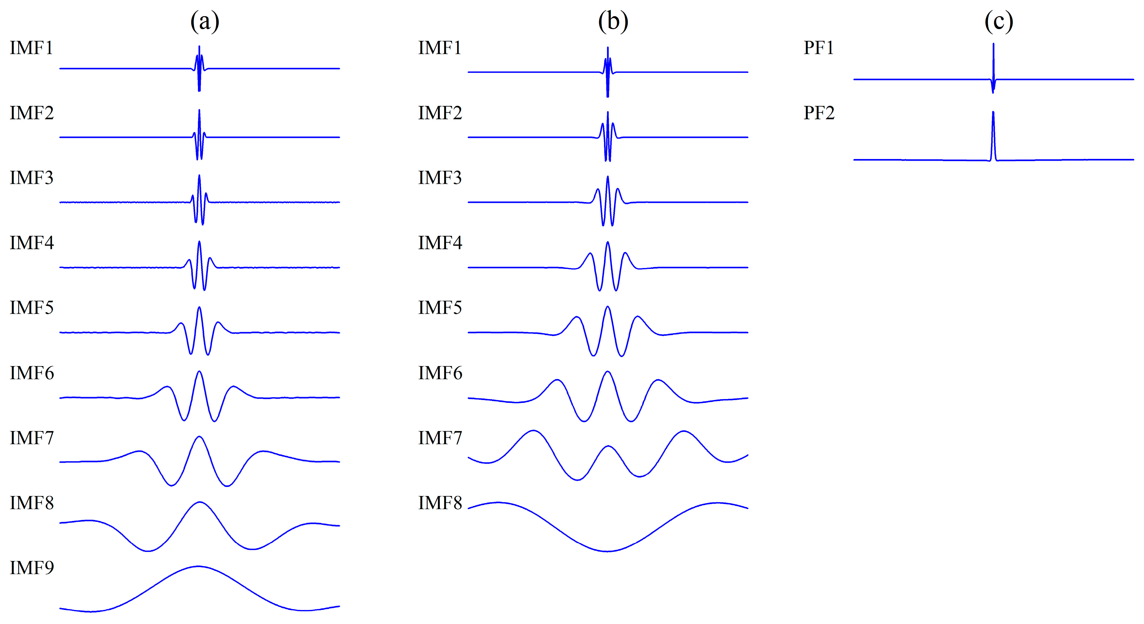
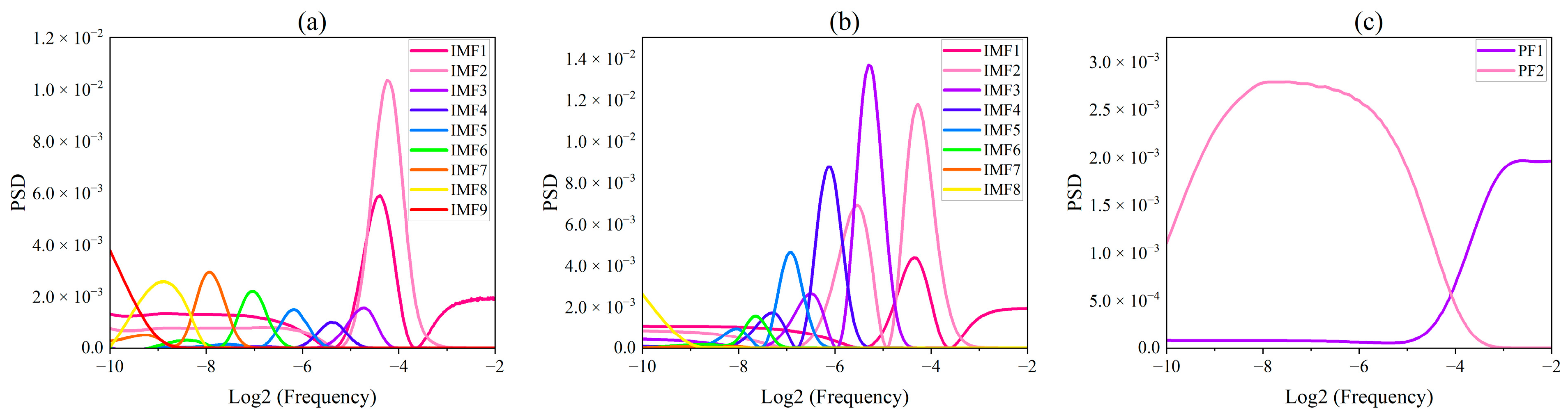
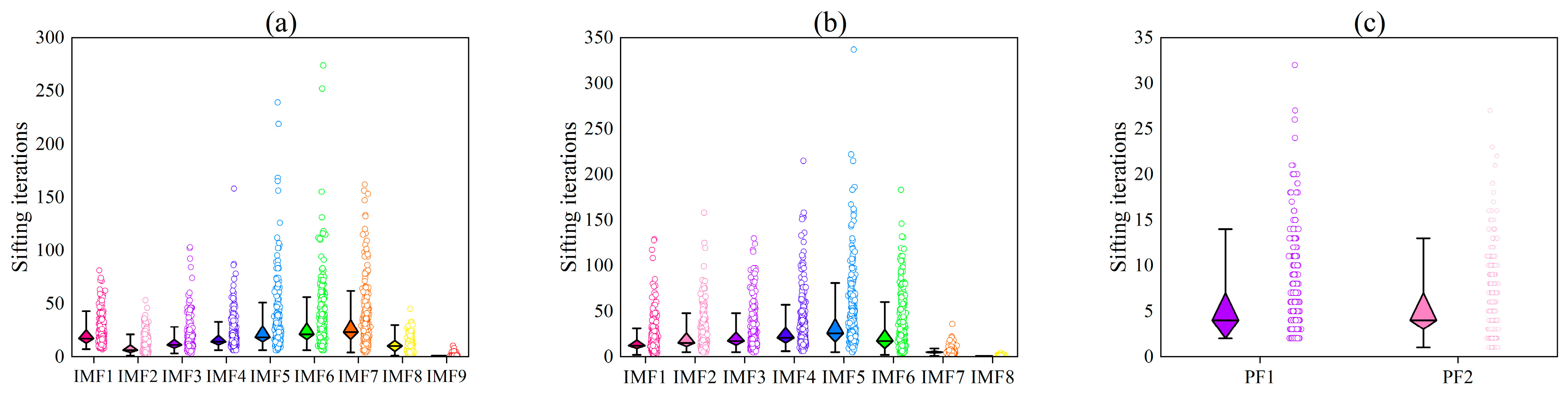
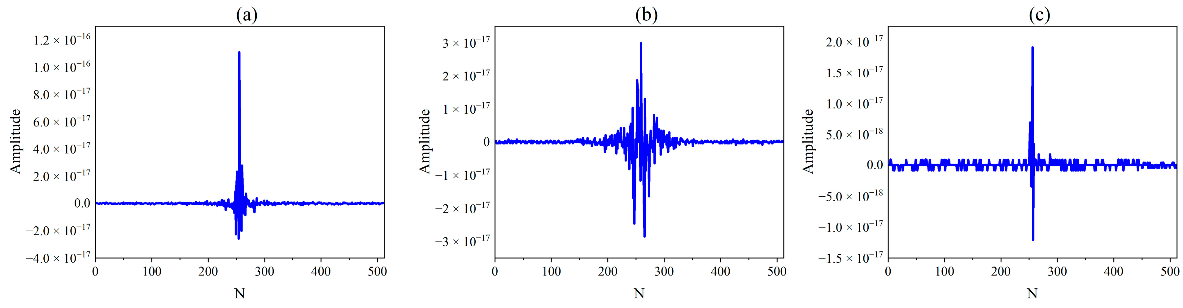
2.3. Impulse Signal Decomposition Experiments

Because most mechanical fault vibration signals, such as rolling element bearing fault signals, contain a large number of impulse signals due to the impact of fault shocks, most scholars often use the Dirac function as an impulse response signal to test the feasibility of empirical modal decomposition methods. The literature [40] compares the decomposition results of the EEMD and CEEMDAN methods for Dirac functions and verifies the advantages of the CEEMDAN method in decomposition ability. So, in this section, we compare the decomposition effects of CEEMDAN, ICEEMDAN, RLMD and CCERLMDAN for Dirac functions $\delta (t)$ with a sample length of 512.

Figure 1 shows the decomposition results obtained for the CEEMDAN, ICEEMDAN, and CCERLMDAN methods, all with the same parameters (SNR = 14 dB). The CEEMDAN method obtained nine modal components, the ICEEMDAN method obtained eight modal components, the method in this paper obtained only two modal components, and the RLMD method could not decompose $\delta (t)$. Compared with the CEEMDAN and ICEEMDAN methods, the CCERLMDAN method obtained fewer modes, indicating that the method outperforms the other two methods in the field of computational efficiency and information aggregation. By observing the decomposed mode component waveforms, the CCERLMDAN method has more compact mode component waveforms, higher component amplitudes and retains more shock features.

To compare the high and low spectral separation properties of the three methods, the power spectral density (PSD) of the modal components obtained by the three methods is given in Figure 2. It is noted that in the CEEMDAN, the overlap between adjacent modal components is serious, especially the overlap between IMF1 and IMF2, which is the most obvious. In the ICEEMDAN method, the energy leakage occurs in IMF7–8, which is barely observed in the power spectrum. Compared with the other two methods, the spectral overlap of each component obtained by the CCERLMDAN method is less, and the separation of frequency components between modes can be clearly displayed.

The number of iterations to compare the three methods is shown in Figure 3. Note the difference in the vertical axis size of the three box diagrams (300 vs. 350 vs. 35, respectively), and the total number of sifting iterations of the three methods are 79,043, 78,859, and 5462, respectively. The number of screening iterations of the proposed method CCERLMDAN accounts for only 7% of CEEMDAN and 6.9% of ICEEMDAN, so this method has a good computational efficiency.

The residual noise in CCERLMDAN and the other two approaches were used for further comparison. The reconstruction errors of the CCERLMDAN and the other two approaches are shown in Figure 4, which are similar in magnitude (orders of 10⁻¹⁶,10⁻¹⁷ and 10⁻¹⁷, respectively), but the CCERLMDAN method is closer to zero.

To make a more precise comparison,

Table 1. The orthogonality and correlation coefficient of the three methods.

Method	IO	Cor1	Cor2
CEEMDAN	0.7936	0.4496	0.4502
ICEEMDAN	0.7504	0.4705	0.3473
CCERLMDAN	0.0365	0.8721	0.5470

shows the outcomes of three approaches for calculating the orthogonality index (IO) and the correlation coefficient (Cor) of the first two modal components. The results show that the IO value of CCERLMDAN is the lowest, so this method can effectively suppress modal mixing. CCERLMDAN has the highest Cor1 and Cor2 among the three methods, which means that the outcome of the decomposition is more consistent with the original signal.

In summary, through the comparison of the above aspects, CCERLMDAN achieves better decomposition accuracy while reducing false components, and obtains a better decomposition performance than CEEMDAN, ICEEMDAN and RLMD.

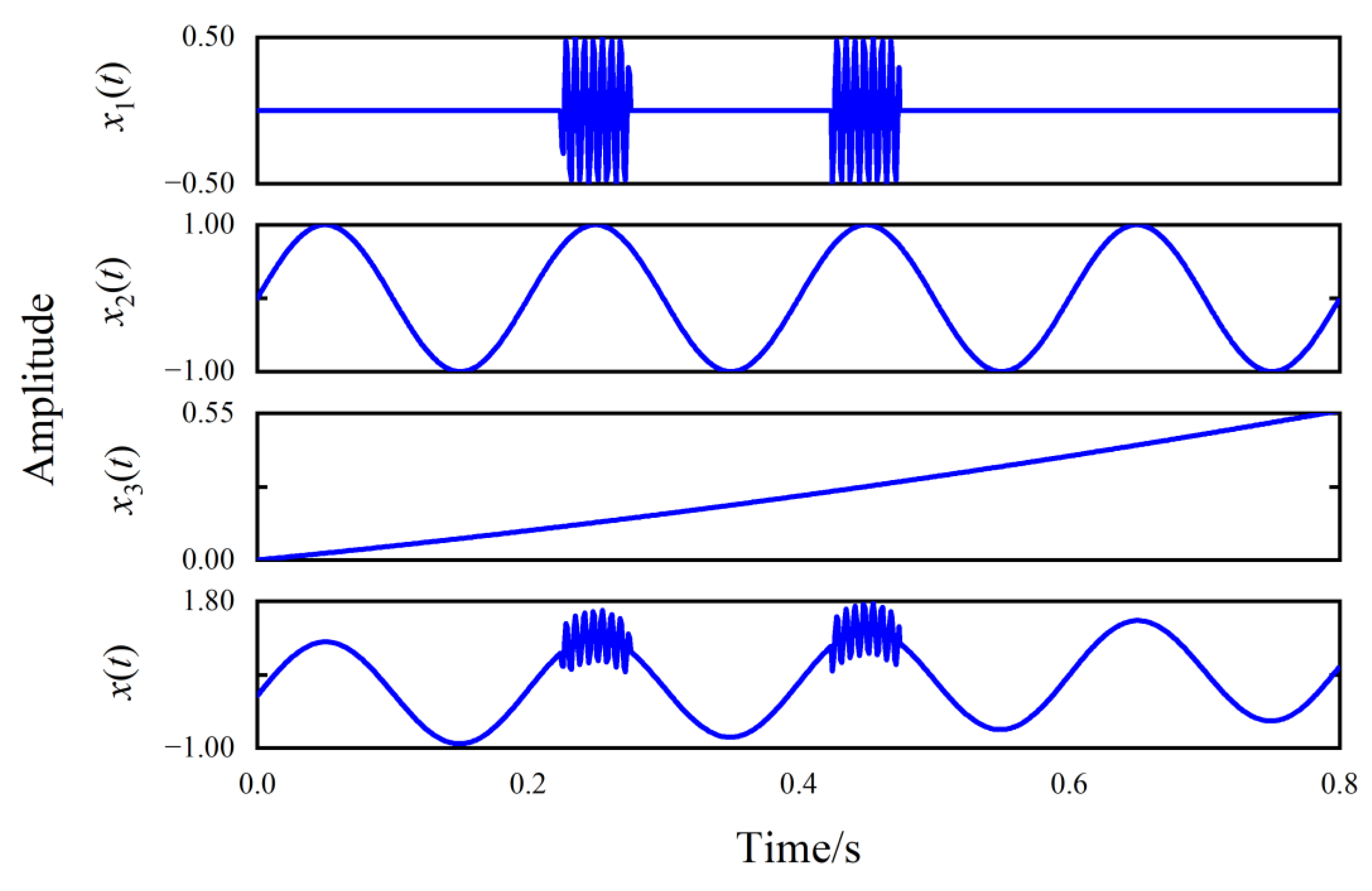
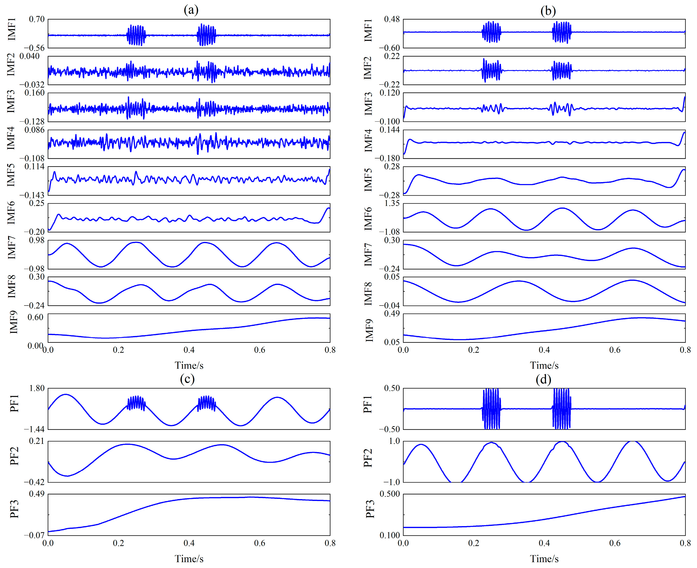
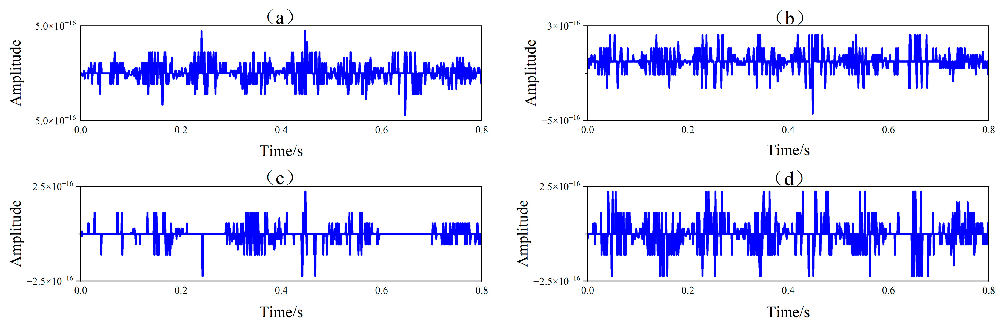
2.4. Synthesis Signal Decomposition Experiments

In this section, the decomposition performance of CEEMDAN, ICEEMDAN, RLMD and CCERLMDAN is further compared by taking the synthetic analog signal as an example. The analog signal $x(t)$ consists of three components $x_1(t)$, $x_2(t)$ and $x_3(t)$, where $x_1(t)$ is an intermittent signal, $x_2(t)$ is a sinusoidal signal and $x_3(t)$ is a quadratic trend signal, and they are expressed as follows:

$$\{\begin{array}{c}\begin{array}{l}{x}_1(t)=0.2\times \sin (150\times 2\times \pi \times t)\times (u(t-0.225)\\ -u(t-0.275)+u(t-0.425)-u(t-0.475))\end{array}\\ x_2(t)=\sin (5\times 2\times \pi \times t)\\ \begin{array}{c}{x}_3(t)=\frac{t}{2}+{(\frac{t}{2})}^2\\ x(t)=x_1(t)+x_2(t)+x_3(t)\end{array}\end{array}$$

(10)

where $u(t)$ is a step function, the sampling rate is set to 1000 and the sampling point is 800. The analog signal $x(t)$ and its three superimposed stimulation signals are shown in Figure 5.

The outcomes of decomposing the analog signal $x(t)$ by the CEEMDAN, ICEEMDAN, RLMD, and CCERLMDAN methods are shown in Figure 6. The CEEMDAN, ICEEMDAN, and CCERLMDAN methods are set to the same parameters ${\beta }_0=0.2$ (SNR is equal to 14 dB) and $I=100$. As illustrated in Figure 6, although CEEMDAN and ICEEMDAN can decompose the synthesis signals adaptively and reflect the real components, there is an obvious mode mixing between modals and multiple false components which symbolize that intermittent signals and sinusoidal signals (such as IMF2–6 and IMF8 of CEEMDAN, IMF2–5 and IMF7–8 of ICEEMDAN) are being generated. Further, as mentioned before, the RLMD showed strong modal mixing when dealing with intermittent signals, and cannot decompose the intermittent signal $x_1(t)$ and the sinusoidal signal $x_2(t)$. In contrast, the CCERLMDAN can further suppress the modal mixing phenomenon and decompose the signal effectively; the decomposition results show good agreement with the intermittent and sinusoidal components, and the quadratic trend signal $x_3(t)$ has less loss compared to other methods. Figure 7 shows the reconstruction errors generated by the four methods in decomposing synthetic signal $x(t)$. Note that the reconstruction errors from all four methods are close to 0 (in the order of 10⁻¹⁶), but the RLMD and CCERLMDAN methods have much smaller errors.

In addition, to better quantify and compare the decomposition ability of the four methods, The IO values and correlation coefficients calculated by the four methods are shown in

Table 2. The orthogonality and correlation coefficient of the four methods.

Method	IO	Cor1	Cor2	Cor3
CEEMDAN	0.1476	0.9818	0.9621	0.9613
ICEEMDAN	0.1419	0.9853	0.9828	0.9489
RLMD	0.1517	0.1627	−0.1353	0.8185
CCERLMDAN	0.0270	0.9973	0.9955	0.9852

. The findings demonstrate that the CCERLMDAN method outperforms the other methods in relation to orthogonality and decomposition accuracy in the decomposition of the simulated signals.

In summary, the CCERLMDAN suppresses the modal mixing problem of RLMD when dealing with intermittent signals under the effect of noise-assisted methods, and produces fewer false components than CEEMDAN and ICEEMDAN. Therefore, this method has a better decomposition ability and decomposition accuracy.

3. Background Theory of MDMVO

3.1. MVO Method

The Multi-Verse Optimizer simulates the transfer of matter through black holes, wormholes and white holes in the universe. The principle simulates the theory that the universe always moves from a high expansion rate to a low expansion rate in a random environment, and promotes the transfer process under the action of the driving force, namely universal gravitation. The process can also be explained as the universe gradually converging on the optimal position in the search space. The iterative process is divided into the global exploration process and local exploitation process. In the whole process, the wormhole acts as a medium, and searches for space through the interaction between the black hole and the white hole. The universe represents the problem’s workable solution, and the expansion rate of the universe represents the fitness value.

3.2. MDMVO Method

Despite the fact that the MVO has fewer parameters and a simple structure, it also has the disadvantages of easily falling into local optimum and premature convergence. The MVO algorithm is improved in this study using population initialization, a nonlinear convergence factor, and multi-disturbance tactics to increase the algorithm’s speed and accuracy during convergence. Among them, the multi-disturbance strategy is the division framework suitable for the early, middle and late search of the algorithm, which are Cauchy mutation, Gaussian mutation and Lévy flight. A schematic of the algorithm framework is shown in Figure 8f.

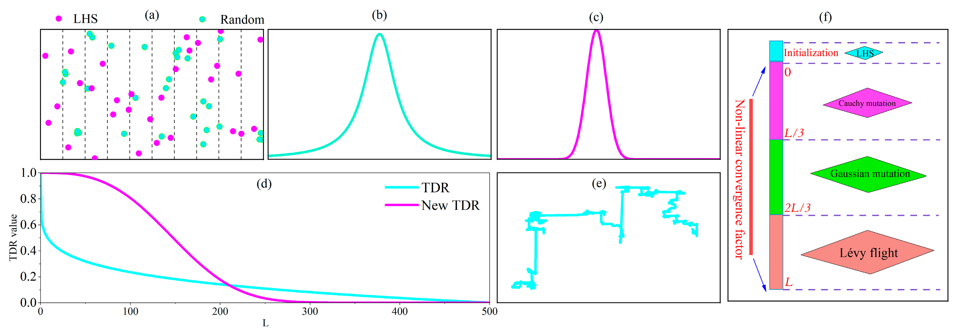
3.2.1. Latin Hypercube Sampling

The MVO algorithm population initialization uses random sequence generation, which can easily lead to population diversity and the irrational distribution of the population search space. In contrast, Latin hypercube sampling (LHS) is a stratified random sampling method, the principle of which is to sample effectively from the distribution intervals of the variables. Assuming that there are $k$ population variables $x_1,x_2,\dots x_k$, we first extract N samples from a specific interval, and then the memory distribution of each variable is divided into N micro-intervals of the same size. A value is randomly selected from each interval, and the N values in each variable are randomly combined with the values of other variables. Compared with other sampling methods, this sampling method enables each edge distribution to be stratified, allowing full coverage of the search space to be achieved for each variable. Therefore, Latin hypercube sampling is applied to the initialization of the algorithm, allowing the initial population of individuals to cover the search space as much as possible to increase the initial population’s diversity, thereby improving the algorithm’s search efficiency.

As observed in Figure 8a, when the original MVO algorithm initializes the population in a random manner, the distribution of the population is relatively concentrated, and there are fewer individuals of the universe in the edge region, so the diversity of the population is small. The population obtained by Latin hypercube sampling is more evenly distributed throughout the search space.

3.2.2. Nonlinear Convergence Factor

In the MVO algorithm, the optimization of the algorithm primarily relies on black holes to journey around the optimal universe and explore, based on wormholes, the travel distance rate (TDR), which has an inverse relationship with the number of iterations, and is a crucial variable to coordinate the algorithm’s ability to explore and develop. It is also the key factor determining the MVO algorithm’s search optimality. The capacity for global exploration is better served by a high TDR value, whereas the capability for local deep mining is better served by a low TDR value. Therefore, to retain the fast global search capabilities of early iterations and the better local exploitation capabilities of later iterations, the TDR is updated to Equation (11), where $L$ is the maximum number of iterations and $l$ is the number of iterations that have already been reached. The comparison of the two travel distance rates is shown in Figure 8d.

$$TDR=\exp (-{(\frac{3l}{L})}^3)$$

(11)

3.2.3. Cauchy Mutation

As shown in Figure 8b, The Cauchy mutation is a continuous probability distribution, common in probability theory, with a higher probability density at the origin, a smaller density at the ends, and a long, flat shape. It is for this reason that features can produce large disturbances to the universe of individuals by incorporating Cauchy mutation, enabling the algorithm to leave the local optimum with less difficulty. Equation (12) provides the common formula for the Cauchy mutation probability density function.

$$C(x)=\frac{1}{\pi }\times \frac{1}{(x^2+1)}$$

(12)

Since the Cauchy mutation decreases from the peak to both sides, and has a relatively flat and small peak, the universe population will spend less time searching the adjacent space after the mutation, and spend its main effort on finding the global optimum. The global optimum obtained from the search space is mutated using Cauchy mutation, as in Equation (13), where $C(x)$ is the Cauchy mutation.

$$X_n=X(j)+X(j)\times C(x)$$

(13)

3.2.4. Gaussian Mutation

From the probability distribution of the Gaussian distribution, it is clear that the Gaussian mutation strategy is an individual neighborhood exploited in depth, which aids in the enhancement of the solution’s convergence accuracy. Therefore, during the iteration of MVO, Gaussian mutation is performed on the individual position of the universe, and the position with the highest fitness is chosen as best universe position after comparing the positions before and after the mutation. The formula is given in Equation (14), and the shape is shown in Figure 8c where $Gauss(0,1)$ is a random variable of the Gaussian distribution.

$$X_n=X(j)+X(j)\times Gauss(0,1)$$

(14)

3.2.5. Lévy Flight

Lévy flight is a non-Gaussian walking model derived from chaos theory. Its main principle is to simulate the flight behavior of insects in nature; the flight process includes short-distance exploitation and long-distance exploration, and the diversity of its activities effectively prevents the algorithm from converging too early. Its mathematical model is described as Equations (15)–(17), where $\mu$ and $v$ are normally distributed, $\beta$ is an important parameter for adjusting the stability of Lévy’s flight, and is taken to be 1.5 in this paper. Applying the Lévy flight to the MVO algorithm updates the universe position, as in Equation (18), where $L(\lambda )$ is the Lévy flight.

The trajectory of the Lévy flight is shown in Figure 8e. The trajectory is a random wandering, and most likely in the form of large strides. The direction of the next movement and the speed of flight are random and unpredictable.

$$Levy(\lambda )=\alpha \times \frac{\mu \times \sigma }{|\nu {|}^{\frac{1}{\beta }}}$$

(15)

$$\lambda =\beta +1$$

(16)

$$\sigma =\left(\frac{\Gamma (1+\beta )\times \sin \left(\frac{\pi \beta }{2}\right)}{\Gamma \left(\frac{1+\beta }{2}\right)\times \beta \times 2\left(\frac{\beta -1}{2}\right)}\right)$$

(17)

$$X_n=X(j)+X(j)\times L(\lambda )$$

(18)

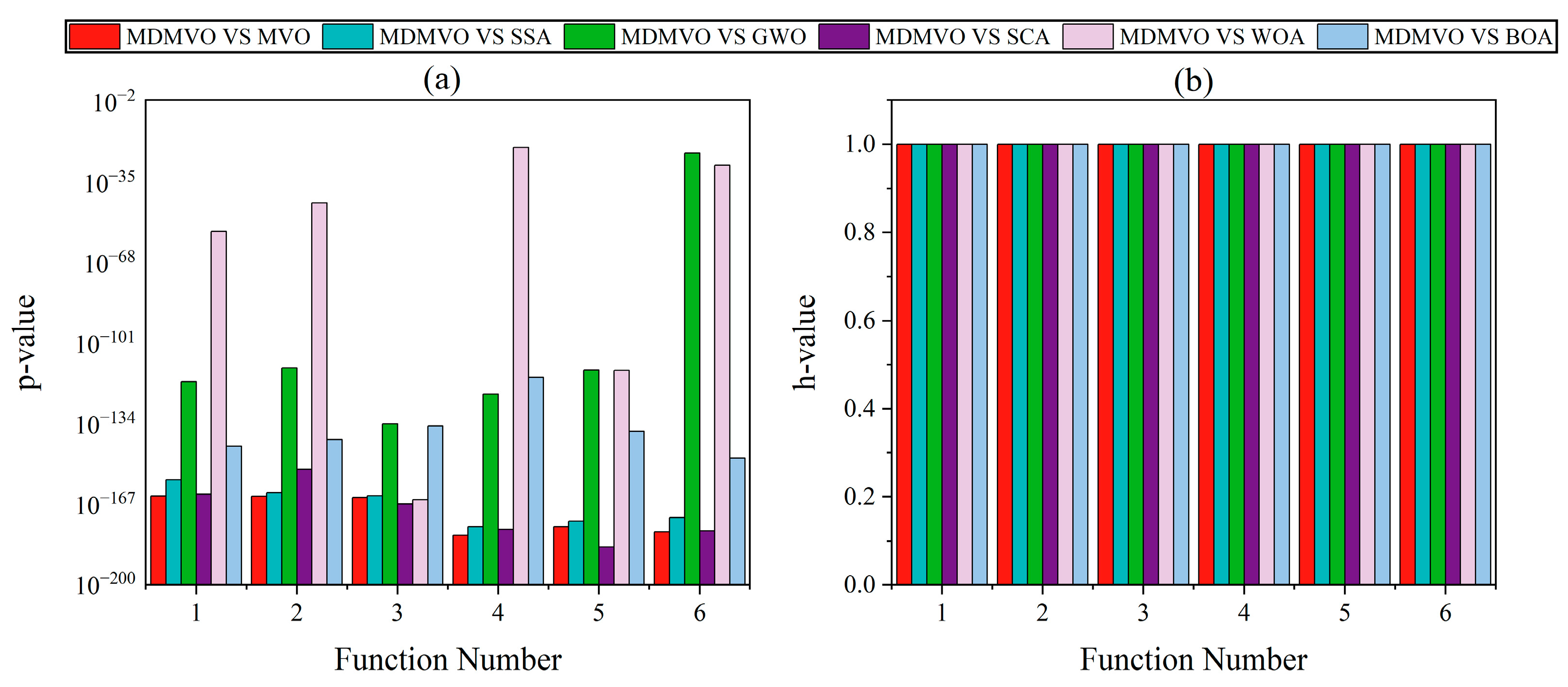
3.2.6. Evaluation of the Exploitation Ability of MDMVO

To evaluate the MDMVO algorithm performance in terms of convergence, as well as optimization-seeking accuracy, six test functions were chosen for experimental comparison, which included unimodal functions $F_1-F_3$ and multimodal functions $F_4-F_6$. The test functions are listed in

Table 3. Unimodal test functions and Multimodal test functions.

Function	Dim	Range	${\mathit{f}}_{\mathbf{min}}$
$F_1(x)={\displaystyle {\sum }_{i=1}^n{x}_i^2}$	30	[−100, 100]	0
$F_2(x)={\displaystyle {\sum }_{i=1}^n\left|x_i\right|}+{\prod }_{i=1}^n\left|x_i\right|$	30	[−10, 10]	0
$F_3(x)={\max }_i\left\{\left|x_i\right|,1\le i\le n\right\}$	30	[100, 100]	0
$F_4(x)={\displaystyle {\sum }_{i=1}^n\left[x_i^2-10\cos (2\pi x_i)+10\right]}$	30	[−5.12, 5.12]	0
$F_5(x)=-20\exp (-0.2\sqrt{\frac{1}{n}{\displaystyle {\sum }_{i=1}^n{x}_i^2}})-\exp (\frac{1}{n}{\displaystyle {\sum }_{i=1}^n\cos (2\pi x_i)})+20+e$	30	[−32, 32]	0
$F_6(x)=\frac{1}{4000}{\displaystyle {\sum }_{i=1}^n{x}_i^2}-{\prod }_{i=1}^n\cos (\frac{x_i}{\sqrt{i}})+1$	30	[−600, 600]	0

. The Whale Optimization Algorithm (WOA), the Multi-Verse Optimizer (MVO), the Salp Swarm Algorithm (SSA), the Grey Wolf Optimization Algorithm (GWO), the Sine Cosine Optimization Algorithm (SCA), and the Butterfly Optimization Algorithm (BOA) were selected for comparison experiments. Each algorithm was run 30 times independently with a maximum iteration count of 500, and population size of 30.

Table 4. The findings from tests on unimodal and multimodal functions.

ID	Metric	MDMVO	MVO	SSA	GWO	SCA	WOA	BOA
	Best	0.00 × 100	0.58 × 100	2.51 × 10−8	5.94 × 10−28	0.01 × 100	1.10 × 10−82	1.03 × 10−11
F1	AVG	0.00 × 100	1.19 × 100	1.61 × 10−7	7.30 × 10−26	3.01 × 101	2.38 × 10−74	1.25 × 10−11
	SD	0.00 × 100	0.39 × 100	3.56 × 10−7	1.57 × 10−25	7.30 × 101	9.02 × 10−74	1.09 × 10−12
	Best	2.20 × 10−170	0.43 × 100	0.45 × 100	8.62 × 10−17	1.91 × 10−4	8.03 × 10−59	2.25 × 10−9
F2	AVG	4.21 × 10−152	0.89 × 100	2.16 × 100	6.69 × 10−16	0.02 × 100	2.36 × 10−51	4.86 × 10−9
	SD	1.30 × 10−151	0.35 × 100	1.44 × 100	4.28 × 10−16	0.03 × 100	8.35 × 10−51	9.49 × 10−10
	Best	1.26 × 10−174	1.04 × 100	3.97 × 100	9.01 × 10−8	7.77 × 100	1.55 × 100	5.36 × 10−9
F3	AVG	2.39 × 10−150	1.95 × 100	1.11 × 101	6.46 × 10−7	3.45 × 101	4.52 × 101	6.21 × 10−9
	SD	7.56 × 10−150	0.79 × 100	3.97 × 100	5.06 × 10−7	1.08 × 101	2.56 × 101	4.37 × 10−10
	Best	0.00 × 100	5.71 × 101	2.19 × 101	5.68 × 10−14	0.02 × 100	0.00 × 100	0.00 × 100
F4	AVG	0.00 × 100	1.24 × 102	5.27 × 101	0.48 × 100	4.42 × 101	0.00 × 100	3.86 × 101
	SD	0.00 × 100	3.02 × 101	1.72 × 101	1.27 × 100	4.12 × 101	0.00 × 100	7.78 × 101
	Best	8.88 × 10−16	1.05 × 100	1.50 × 100	7.90 × 10−14	8.56 × 100	8.88 × 10−16	3.70 × 10−9
F5	AVG	8.88 × 10−16	2.33 × 100	2.42 × 100	1.56 × 10−13	1.41 × 101	4.20 × 10−15	5.93 × 10−9
	SD	0.00 × 100	3.28 × 100	0.59 × 100	4.52 × 10−14	0.04 × 100	2.27 × 10−15	7.68 × 10−10
	Best	0.00 × 100	0.68 × 100	0.01 × 100	0.00 × 100	0.02 × 100	0.00 × 100	7.13 × 10−13
F6	AVG	0.00 × 100	0.85 × 100	0.02 × 100	0.01 × 100	0.89 × 100	0.01 × 100	4.55 × 10−12
	SD	0.00 × 100	0.07 × 100	0.02 × 100	0.01 × 100	0.34 × 100	0.04 × 100	2.43 × 10−12

displays the best results, mean, and standard deviation for each algorithm after 30 independent runs, the optimal results have been expressed in bold.

Based on the experimental findings, it can be seen that the MDMVO algorithm proposed in this paper outperforms other algorithms according to average, best value and standard deviation of the optimization results of all test functions. For the unimodal functions $F_2$ and $F_3$, MDMVO is significantly higher than the other algorithms in order of magnitude, although it does not find the optimal value of 0. For the functions $F_1$, $F_4$ and $F_6$, the MDMVO algorithm finds the theoretical best value of 0. For the function $F_5$, the MDMVO algorithm finds the general best value, 8.88 × 10⁻¹⁶, of the function.

As can be seen from Figure 9, since the MDMVO method uses Latin hypercube sampling, it provides a basis for the algorithm to find a better initial value than other algorithms, which is very obvious for all function results. With the increase in iterations, the global search ability of the algorithm is improved through Cauchy mutation, Gaussian mutation and Lévy flight. Compared with other comparison algorithms, the algorithm does not fall into local optimum. For functions $F_4$ and $F_6$, the MDMVO algorithm converges faster than the WOA algorithm, which also finds the optimal value.

In order to further compare the obvious differences between the MDMVO algorithm and other algorithms, results from the Wilcoxon rank-sum test for each function are shown in Figure 10, with a significance level of 5%. In this figure, the h values are all equal to 1, and the p values for the MDMVO compared to the MVO, SSA, GWO, SCA, WOA, and BOA are less than 0.05. The findings indicate that the pairwise Wilcoxon rank-sum test was successful, and compared to MVO, SSA, GWO, SCA, WOA and BOA, the MDMVO algorithm shows a statistically superior performance.

In conclusion, the MDMVO algorithm has a better optimization performance, faster convergence speed and a higher stability than the MVO algorithm. The pseudocode of MDMVO is displayed in Algorithm 1.

Algorithm 1. The pseudocode for MDMVO algorithm.

Assign values for parameters $WE{P}_{\max }$, $WE{P}_{\min }$, $p$, $L$ and $n$, $d$, $l$

Define objective function $f(x)$

Latin hypercube sampling initial Multi-Verse population

Get the current optimal universe $x_{best}$

While $l<L+1$

Update $WEP$ and $TDR$

For $j=1:n$

Calculate the inflation rate (fitness) of universes

if $l\le L/3$

Create the new Position of universes $x_n$ using Equation (13)

if $x_n$ better than $x(j)$

$x(j)=x_n$

end if

if $L/3<l<2L/3$

Create the new Position of universes $x_n$ using Equation (14)

If $x_n$ better than $x(j)$

$x(j)=x_n$

end if

if $l\ge 2L/3$

Create the new Position of universes $x_n$ using Equation (18)

if $x_n$ better than $x(j)$

$x(j)=x_n$

end if

for $n=1:d$

Calculate the random variable $r1,r2,r3,r4$ and update the Position of the universes

end for

Update the convergence curve

end for

$l=l+1$

End

4. Proposed Method

4.1. Maximum Correlated Kurtosis Deconvolution (MCKD)

The MCKD approach selects an appropriate filter for the deconvolution computation iteratively to maximize the correlated kurtosis, and extracts the periodic impulse component of the signal. The correlated kurtosis expression is shown in Equation (19), where $y_n$ is the output signal:

$$K_c(T)={\max }_f\frac{{\displaystyle \sum _{n=1}^N{\left({\displaystyle \prod _{m=0}^M{y}_{n-mT}}\right)}^2}}{{\left({\displaystyle \sum _{n=1}^N{y}_n^2}\right)}^{M+1}}$$

(19)

The derivative of Equation (19) is set to zero to determine the best filter $f$, which results in Equation (20):

$$\frac{d}{d{f}_k}{K}_c(T)=0,\hspace{1em}k=1,2,\dots ,L$$

(20)

The combination of the coefficients of the filter vector is represented by Equation (21):

$$f=\frac{{\Vert y_n\Vert }^2}{2\Vert \beta {\Vert }^2}{\left(X_0{X}_0^{\mathrm{T}}\right)}^{-1}{\displaystyle \sum _{m=0}^M{X}_{mT}}{\alpha }_{mn}$$

(21)

where the parameters are shown in Equations (22)–(24):

$$X_{mT}={\left[\begin{array}{ccccc}{x}_{1-mT}& x_{2-mT}& x_{mT}& \dots & x_{N-mT}\\ 0& x_{1-mT}& x_{2-mT}& \dots & x_{N-mT-1}\\ 0& 0& x_{1-mT}& \dots & x_{N-mT-2}\\ ⋮& ⋮& ⋮& & ⋮\\ 0& 0& 0& \dots & x_{N-mT-(L-1)}\end{array}\right]}_{L\times N}$$

(22)

$$\beta ={\left[\begin{array}{c}{y}_1{y}_{1-T}\dots y_{1-MT}\\ y_2{y}_{2-T}\dots y_{2-MT}\\ ⋮\\ y_N{y}_{N-T}\dots y_{N-MT}\end{array}\right]}_{N\times 1}$$

(23)

$${\alpha }_m={\left[\begin{array}{ccc}{y}_{1-mT}^{-1}(y_1^2& y_1^2-T\dots & y_{1-mT}^2)\\ y_{2-mT}^{-1}(y_2^2& y_{2-T}^2\dots & y_{2-mT}^2)\\ ⋮& & \\ y_{N-mT}^{-1}(y_N^2& y_{N-T}^2\dots & y_{N-mT}^2)\end{array}\right]}_{N\times 1}$$

(24)

4.2. MDMVO-Based MCKD

The inverse of the squared Crest Factor of the MCKD deconvolution signal is chosen as the fitness function for the MDMVO to find the optimum. If the fitness function value $FV$ is smaller, the crest factor will be larger, the periodic shock characteristics of the vibration signal will be stronger, and the fault characteristics will be more obvious. The fitness function $FV$ is given in Equation (26), where $C$ is the Crest Factor, $x_p$ is the Crest of the signal, and $x_{rms}$ represents the signal’s root mean square value.

$$C=\frac{x_p}{x_{rms}}$$

(25)

$$FV=1/C^2$$

(26)

Define the range of the filter length $L$, the deconvolution period $T$ and the filter shifts $M$ in the MCKD method influence parameters as the universe search space of the MDMVO algorithm, and $F{V}_i=[L_i,T_i,M_i]$ is the position of the universe. The adaptive process for the parameters $L$, $T$ and $M$ is as for Algorithm 2.

Algorithm 2. MDMVO-based MCKD

Step 1: Define the initial parameters of the MDMVO algorithm and the MCKD influence parameter search interval. set the universe population size to 20, the maximum number of iterations to 30, the MDMVO algorithm wormhole existence probability $WE{P}_{\min }$ to 0.2 and $WE{P}_{\max }$ to 1. The sampling frequency is $f_s$. The fault characteristic frequency $f$, fault period $T=f_s/f$ and fault pulse interval $△T=1/f$ of each component of the bearing are calculated according to the bearing parameters. Set the MCKD method parameters $L\in [10,500]$, $M\in [1,7]$, $T\in [f_s/f-10,f_s/f+10]$.

Step 2: Initialize the position of the universe, obtain the best universe $U_{best}$ and the position of the best universe $F{V}_{best}$.

Step 3: Update the wormhole existence probability $WEP$ and travel distance rate $TDR$, compare the universe expansion rate value during the iteration, and update the optimal universe expansion rate if the rate of the universe’s expansion is higher than it currently is; otherwise, keep the universe as it is. Update the best universe individual $U_{best}$ and the best universe position $F{V}_{best}$.

Step 4: If the condition that the universe is best or if the maximum iteration has been achieved, output the best solution, otherwise go to step 3.

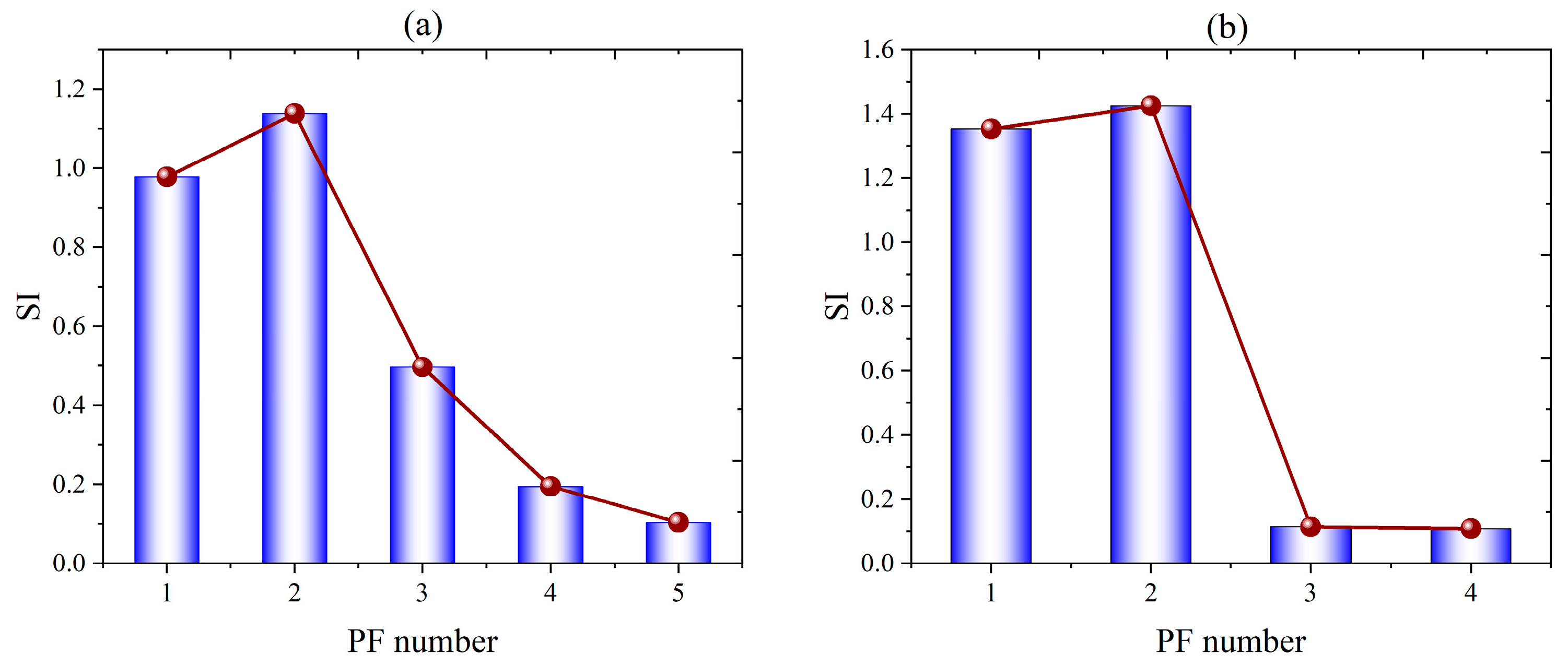
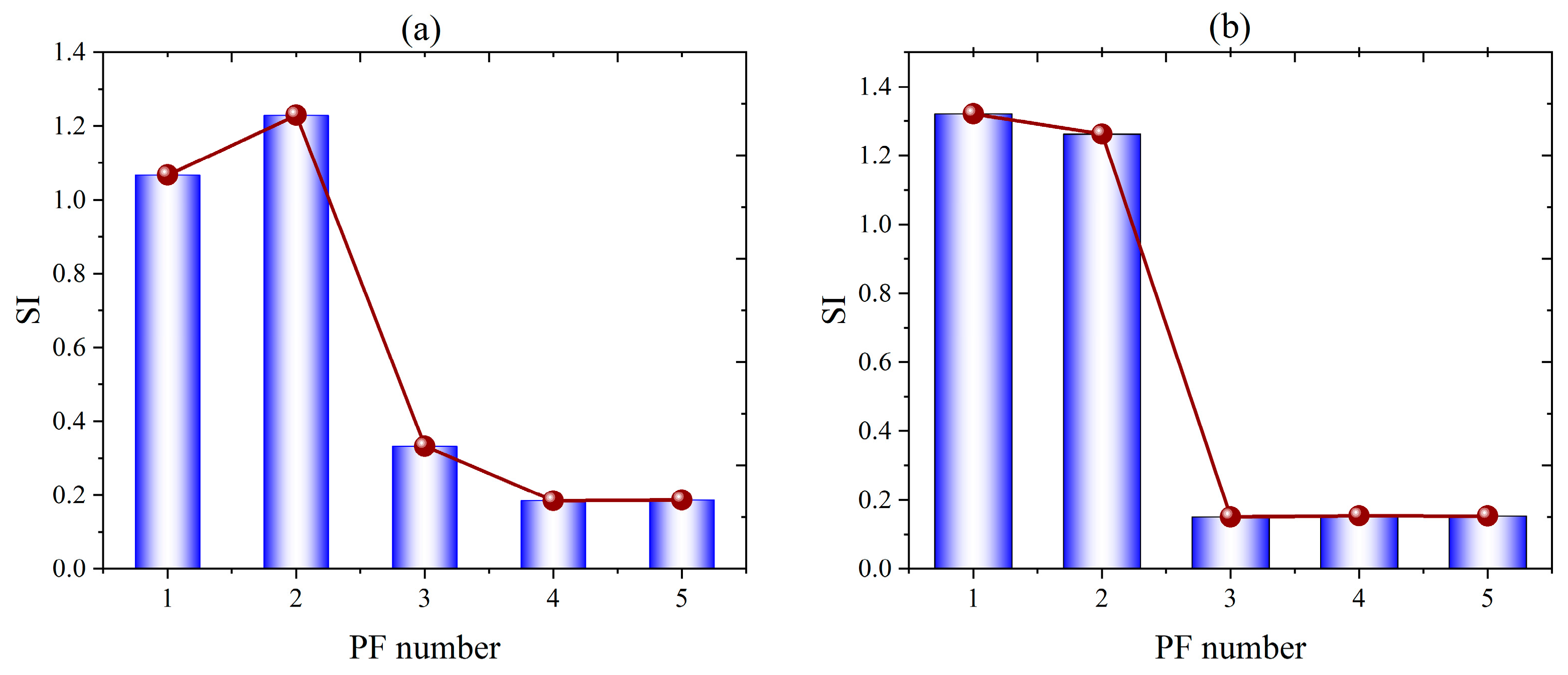
4.3. Selection of Sensitive PF

The selection of modal components in fault diagnosis is also particularly important for the acquisition of fault information. Due to the presence of false components, only a few modal components contain fault information [41]. Most studies to date have adopted the maximum kurtosis principle for the selection of modal components. Despite the fact that kurtosis is especially susceptible to shock signals, kurtosis is also sensitive to disturbances from other external sources and is not suitable for modal component selection when particularly influenced by noisy environments. Multi-scale fuzzy entropy (MFE) is derived from the improved sample entropy and can describe the irregularity and complexity of time series under different scale factors. However, the results of MFE entropy are affected by its embedding dimension and the width of the fuzzy function boundary. Directly using it to select the PF component will also lead to unstable results. The correlation coefficient (CC) reflects the similarity between signals; it is also one of the most commonly used indicators in PF selection. However, when there is a complex non-simple linear correlation between signals, the CC cannot accurately reflect the similarity between signals. Therefore, we proposed the sensitivity index (SI) based on the combination of MFE, CC and kurtosis to select the components generated by the decomposition method. The formula is as Equations (27)–(32):

$$Kurtosis=\frac{E\left[{(X-\mu )}^4\right]}{{\left(E\left[{(X-\mu )}^2\right]\right)}^2}$$

(27)

$$CC=\frac{{\displaystyle \sum _{n=0}^{\infty }x}(n)y(n)}{\sqrt{{\displaystyle \sum _{n=0}^{\infty }{x}^2}(n){\displaystyle \sum _{n=0}^{\infty }{y}^2}(n)}}$$

(28)

$$FE(m,n,r)=\underset{N\to }{\lim }\left[\ln {\varphi }^m(n,r)-\ln {\varphi }^{m+1}(n,r)\right]$$

(29)

$$y_j(\tau )=\frac{1}{\tau }{\displaystyle \sum _{i={(j-1)}_{\tau }+1}^{j\tau }{x}_i},1⩽j⩽\frac{N}{\tau }$$

(30)

$$MFE=FE(y_j(\tau ))$$

(31)

$$S{I}_i=\frac{\overline{MF{E}_i}}{{\displaystyle \sum _{i=1}^{N}MF{E}_i}}+\frac{Kurtosi{s}_i}{{\displaystyle \sum _{i=1}^{N}Kurtosi{s}_i}}+\frac{C{C}_i}{{\displaystyle \sum _{i=1}^{N}C{C}_i}}$$

(32)

Then, the best K order PF component can be stated as Equation (33):

$$K=\arg \max (SI)$$

(33)

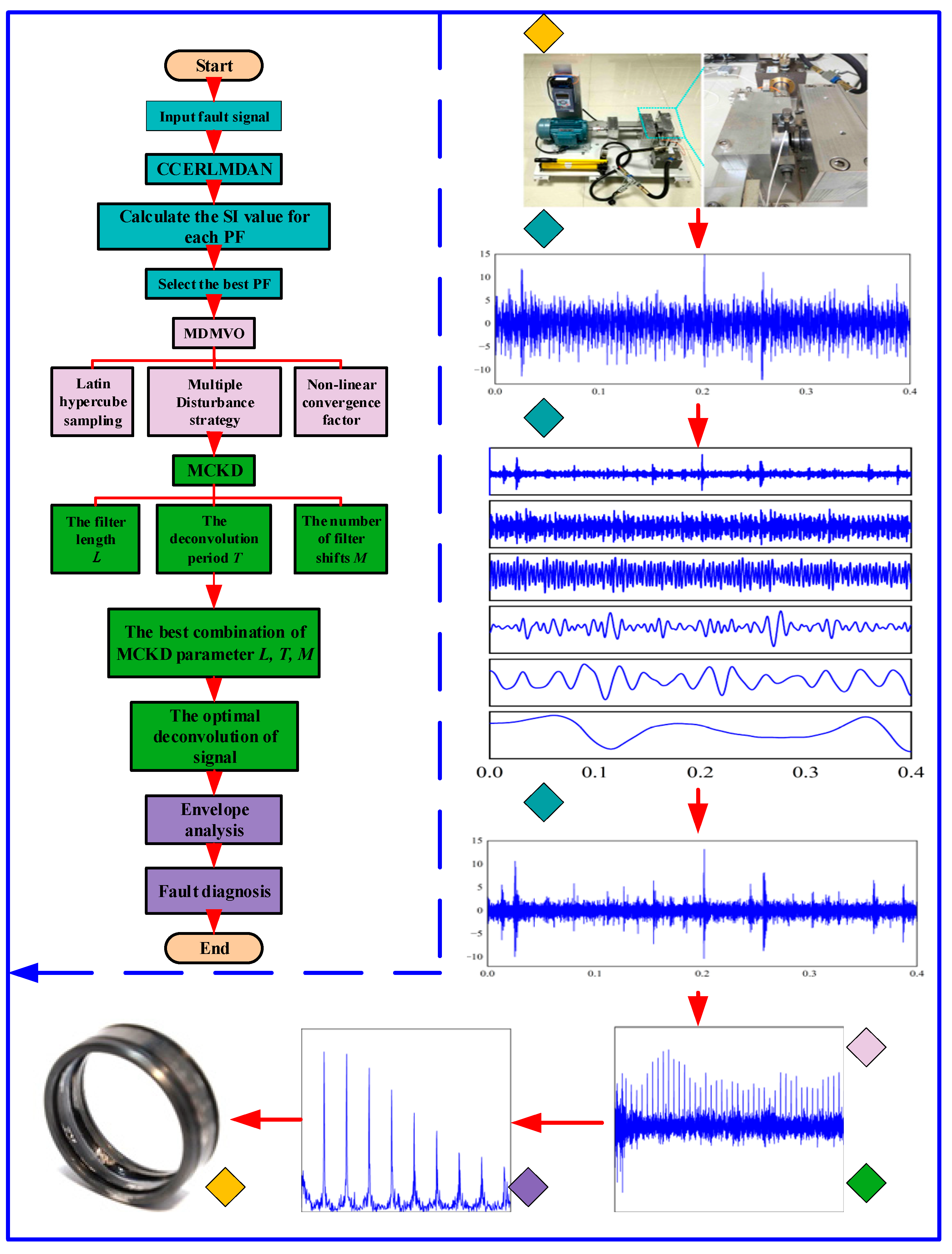
4.4. The Proposed Time—Frequency Method for Diagnosing Rolling Element Bearing Faults

In Section 2 and Section 3, we demonstrated that the proposed CCERLMDAN and MDMVO are more effective than the original method. However, in actual working environments, bearing vibration signals face a more brutal environment, where the information generated by bearing faults is often drowned out by noise, so we need to use relevant methods to enhance the fault information in the signal. Combining all these factors, we propose a novel hybrid fault diagnosis method which combines CCERLMDAN and MDMVO-based MCKD to fully exploit the benefits of the MCKD method in enhancing fault pulse in fault extraction. The method flow is as for Algorithm 3, and also shown in Figure 11.

Algorithm 3. CCERLMDAN and MDMVO-based MCKD

Step 1: The rolling element bearing vibration signal collected by the sensor is decomposed into a series of PF components by CCERLMDAN.

Step 2: The SI value of each PF component is calculated, and the best PF component is selected according to the principle of maximum SI.

Step 3: The MDMVO-based MCKD is used to enhance the fault impulses contained in the selected best PF component and select the best combination of MCKD parameters $L$, $T$ and $M$.

Step 4: Envelope demodulation analysis is used for the best deconvoluted signal in order to extract the bearing fault characteristic frequencies and to determine the fault type.

5. Practical Application

This section will verify the validity of the proposed method in the previous sections by analyzing roller bearing fault signals, where local bearing faults often excite a vibration to produce periodic fault characteristic information. Using established bearing parameters, the formula for calculating the fault frequency of the corresponding position is shown in

Table 5. The characteristic frequency calculation table for different bearing faults.

Calculation formula of inner race fault	$f_{inner}=\frac{N}{2}{f}_r(1+\frac{d}{D}\cos \alpha )$
Calculation formula of outer race fault	$f_{outer}=\frac{N}{2}{f}_r(1-\frac{d}{D}\cos \alpha )$
Calculation formula of roller fault	$f_{roller}=\frac{1}{2}{f}_r[1-{(\frac{d}{D})}^2{\cos }^2\alpha ]\frac{D}{d}$

.

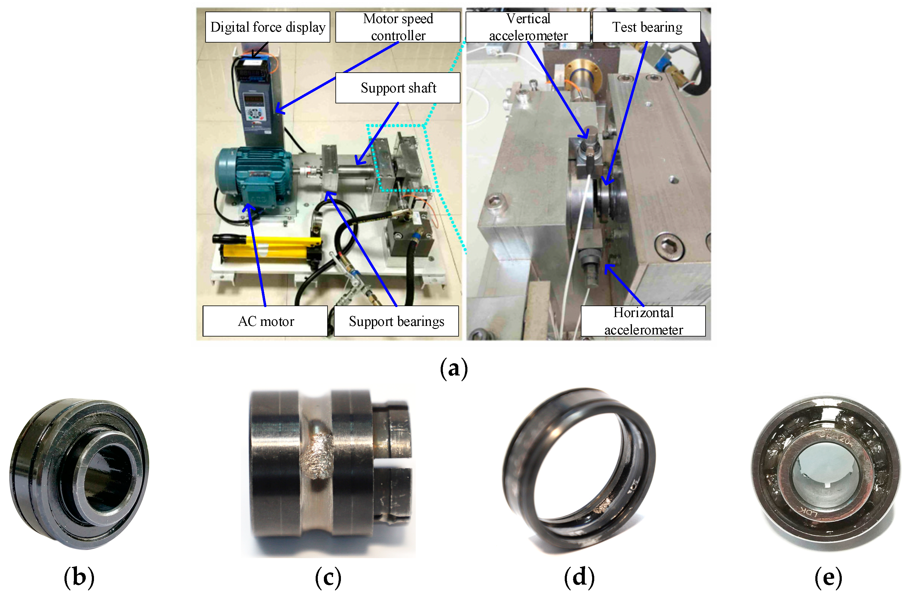
5.1. Data Acquisition

The XJTU-SY rolling element bearing test bench [42] collects rolling element bearing signals. Figure 12 shows the test bench and the rolling element bearings used in the experiment. Magnetic bases are used to fix the two PCB-352C33 acceleration sensors to the horizontal and vertical axes of the test bearing, and the full life cycle fault signal is obtained by adjusting the radial force on the bearing in both the horizontal and vertical directions to be tested, and the speed of the AC motor. The rolling element bearing is an LDK UER204 type, and the diameter of the rolling element, $d$, is 7.92 mm, the diameter of the pitch circle, $D$, is 34.55 mm, the number of rolling elements, $N$, is 8 and the load angle, $\alpha$, is 0 degree. In this study, the data length $N_l$, is 10,240 points, with a sampling frequency $f_s$ of 25.6 kHz.

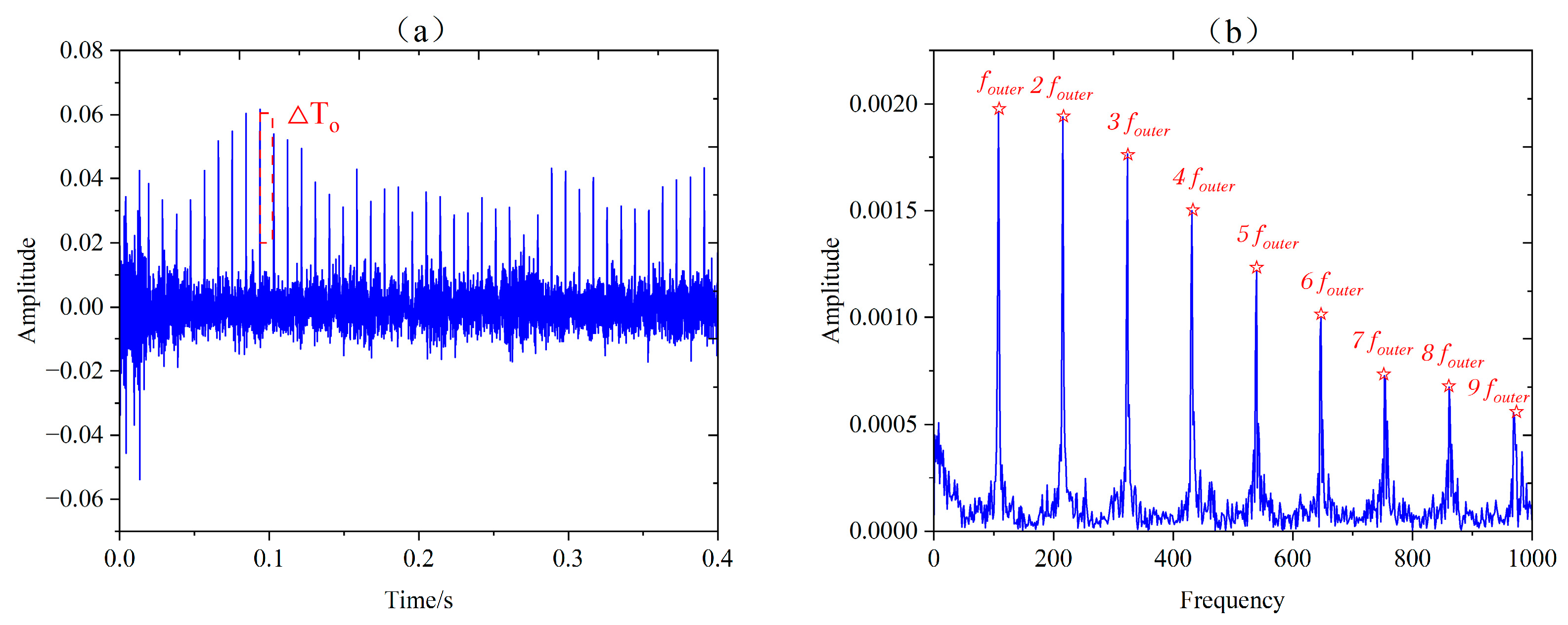
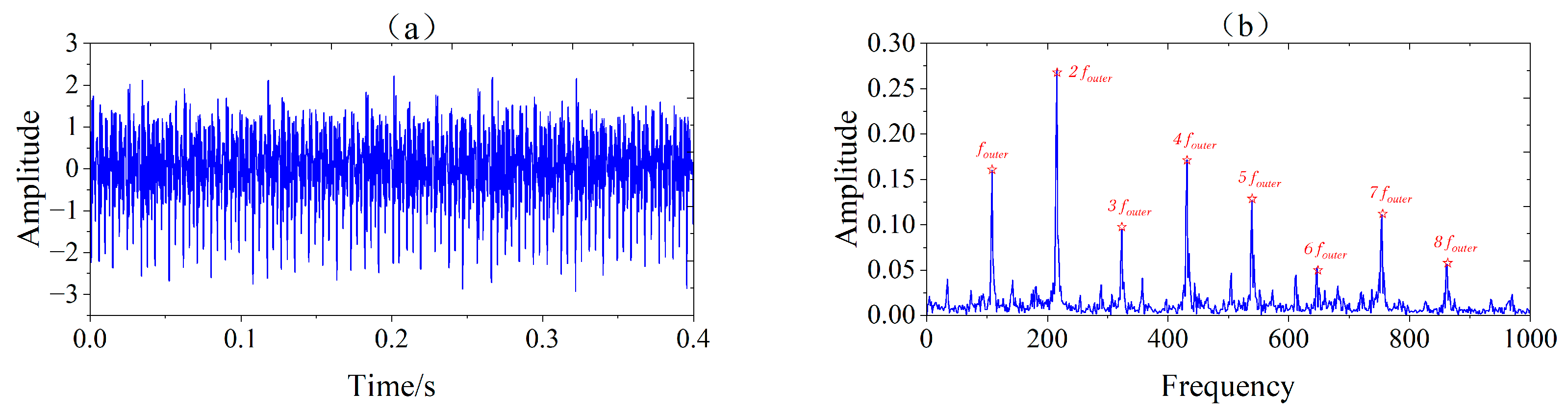
5.2. Experiment and Analysis of Outer Race Fault in Rolling Element Bearings

In this experiment, the motor speed was set to 2100 r/min (The frequency of rotation $f_r$ was 30 Hz) and the bearing outer race was spalled off at the end of the experiment. In light of Table 5, the fault characteristic frequency of the outer race $f_{outer}$ was calculated as 107.91 Hz, the fault period $T_o$ was 237.26, and the fault pulse interval $△T_o$ was 0.0093 s.

Figure 13a displays the bearing outer race failure time domain signal. In the envelope spectrum of Figure 13b, the periodic fault characteristic frequency can be seen. Therefore, noise has less of an impact on the outer race fault signal. This signal is used as a less-disturbed fault signal to compare the decomposition capability of the CCERLMDAN and RLMD methods. The CCERLMDAN setting adds noise with a standard deviation of 0.2 (SNR = 14 dB) and the ensemble number is 100. The SI was calculated according to Equation (33), and is shown in Figure 14. The PF2 component was selected for further envelope analysis according to the principle of maximum SI. Figure 15b depicts the envelope spectrum acquired by the CCERLMDAN approach, while Figure 15a depicts the envelope spectrum obtained by the RLMD method based on the SI. As the figure illustrates, the envelope obtained by the decomposition of the CCERLMDAN method retains more fault characteristic frequency information, while the envelope obtained by the RLMD method can also extract multi-fold fault characteristic frequency information, but the first and sixth harmonics of the fault frequency information ($f_{outer}$, 6$f_{outer}$) are not as evident, since the amplitude of the interference frequency and the resolution is not high, the eighth harmonic of the fault characteristic frequency (8$f_{outer}$) in the envelope spectrum is not seen, so the decomposition effect is poorer than that of CCERLMDAN.

To obtain better fault diagnosis results, the parameter $T\in [227,247]$, and the range of parameters $L$, $M$ in Section 4.2 were set. According to the bearing fault diagnosis approach in this paper, Figure 16 displays the results of processing the bearing outer race fault signal. The best combination of MCKD parameters obtained by this method was [7, 237, 466]. Figure 16a shows the best deconvolution signal for this combination of parameters, where the periodic shock component at intervals of $△T_o$ can be clearly observed, and when compared with the original outer race fault signal, the signal’s kurtosis increases by 4.65 times. The outer race fault characteristic frequency and its ninth harmonic are more prominent in the deconvoluted signal envelope spectrum, as shown in Figure 16b. Compared with the envelope spectrum of the PF2 component, obtained by the CCERLMDAN method, it is clearly obvious that less information exists for the fault characteristic frequency of the outer race (There is a ninth harmonic fault frequency 9 $f_{outer}$).

In conclusion, more fault frequency information can be extracted from the rolling element bearing outer race fault signal using the CCERLMDAN approach than the RLMD approach, and the MDMVO-based MCKD method can adaptively select the best combination of MCKD parameters and achieve better fault frequency extraction results.

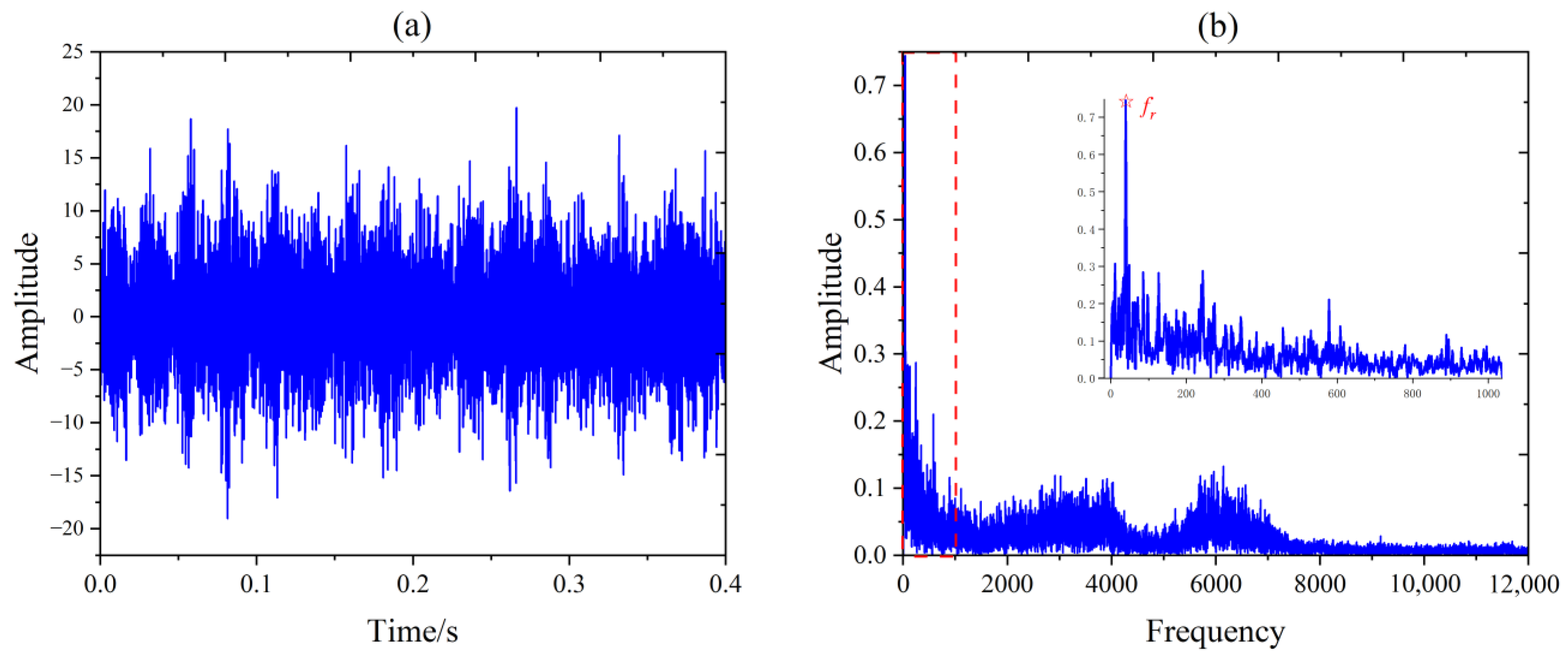
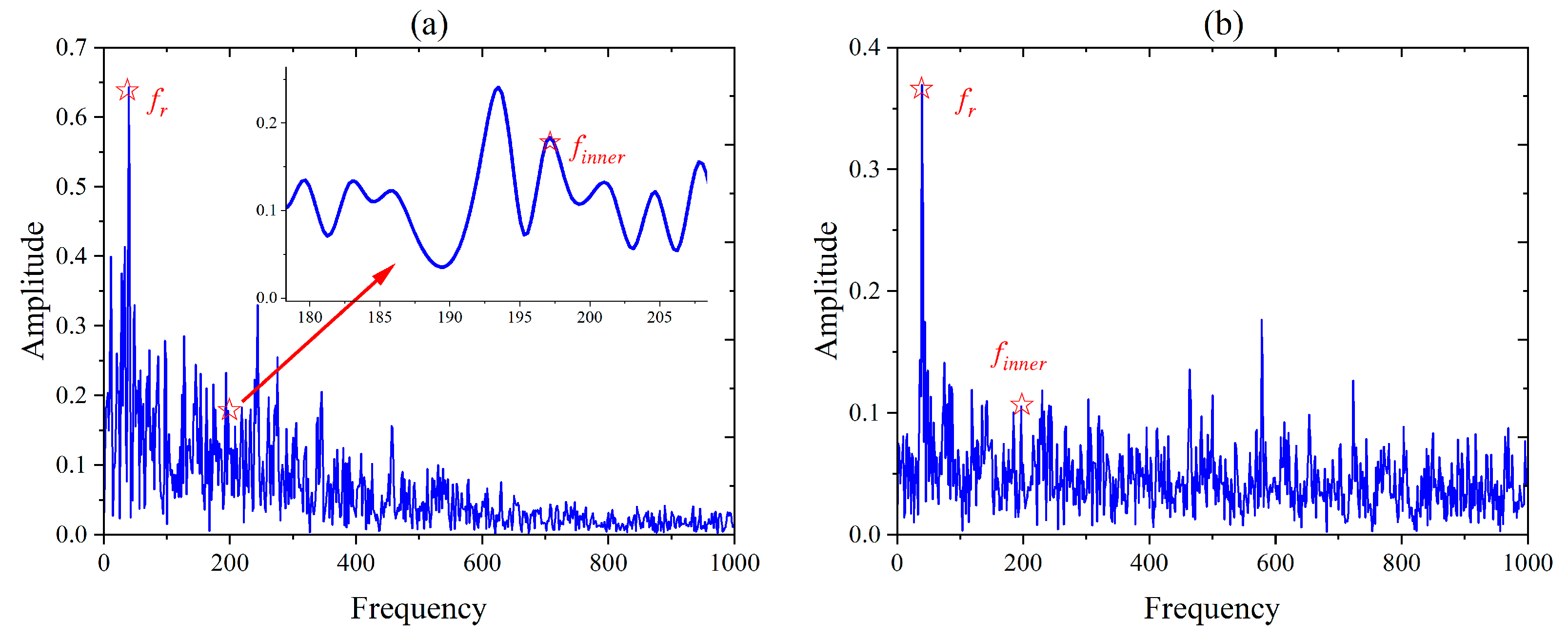
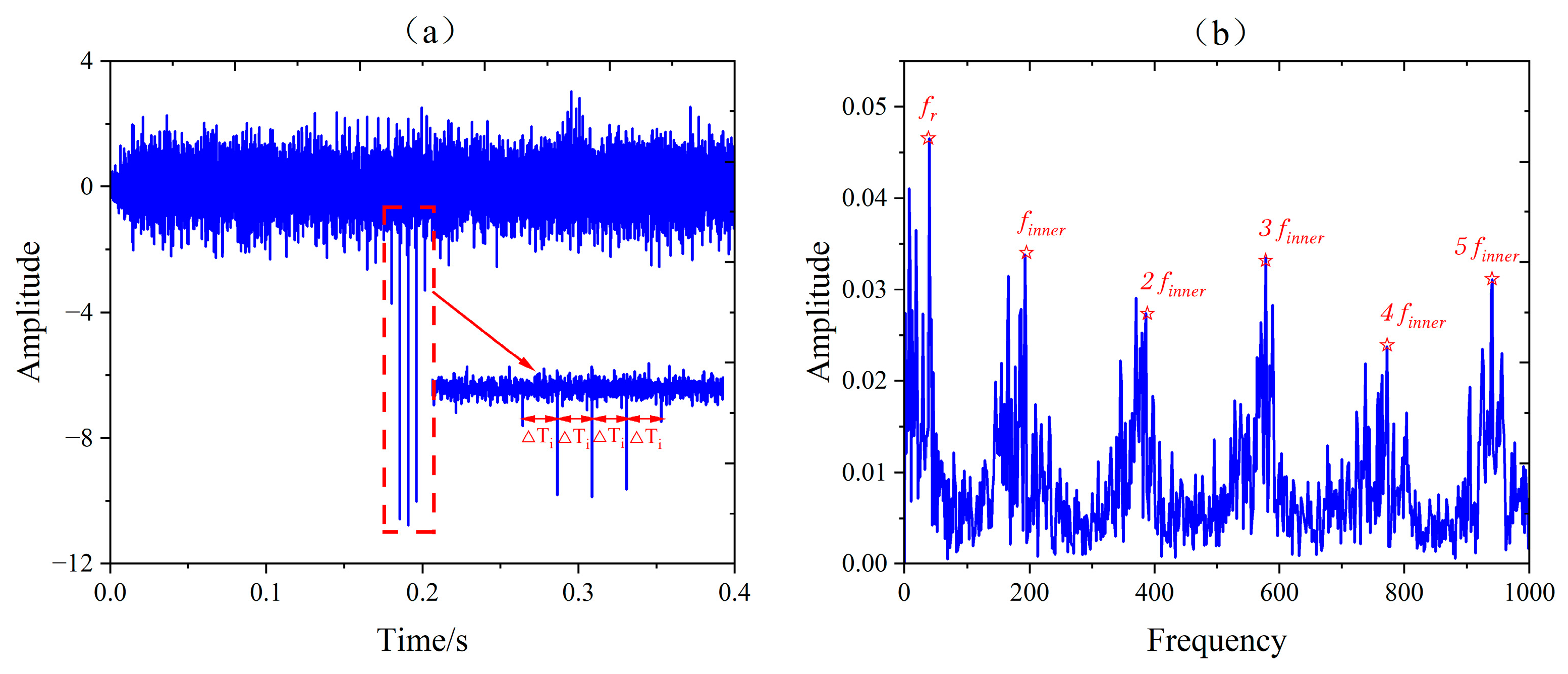
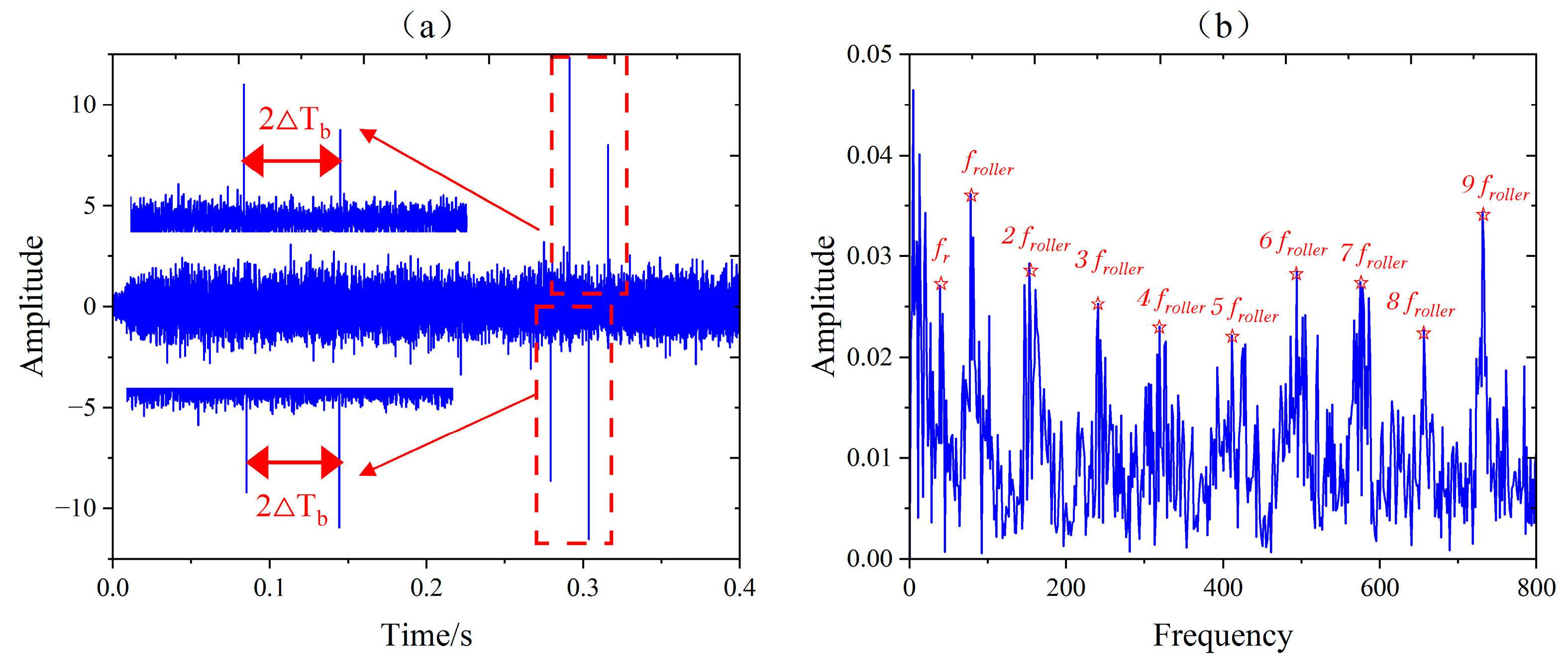
5.3. Experiment and Analysis of Compound Fault in Rolling Element Bearings

In this experiment, the motor speed was set to 2400 r/min (The frequency of rotation $f_r$ is 40 Hz), and at the conclusion of the experiment, the bearing’s inner race, outer race, and roller had failed. According to Table 5, the fault characteristic frequencies of the three different faults were calculated as $f_{inner}$ = 196.68 Hz, $f_{outer}$ = 123.32 Hz, $f_{roller}$ = 82.66 Hz. The fault period is $T_i$ = 130.16, $T_o$ = 207.59, $T_b$ = 309.69, respectively, and the fault pulse interval is $△T_i$ = 0.005, $△T_o$ = 0.008, $△T_b$ = 0.012, respectively.

Figure 17a displays the time domain waveform of the bearing fault signal. In the time domain waveform, the periodic fault pulse is invisible, and the existence of rotational frequency can only be observed in the envelope spectrum Figure 17b, thus it is impossible to locate the fault characteristic frequency of the bearing inner race, outer race, and roller, so the direct spectrum analysis could not determine the bearing fault type or the number of fault sources. The signal is decomposed using the CCERLMDAN and RLMD, and the SI of each PF is then calculated, as shown in Figure 18. In Figure 19a,b, the envelope spectrum of the PF1 component of the RLMD and the CCERLMDAN is displayed, respectively. The inner race fault characteristic frequency can be clearly extracted from the envelope spectrum of CCERLMDAN, while the frequency of inner race fault and interference frequency in the envelope spectrum obtained by the RLMD method are mixed, and the amplitude is not as large as the interference frequency, making the distinction difficult. Therefore, the CCERLMDAN method still has a better decomposition capability than the RLMD method in the case of more severe interference in the time domain of compound fault. However, the two decomposition methods are still unable to determine the type of bearing fault and the number of fault sources, and further processing of the PF is required.

Due to the different fault periods corresponding to each type of fault in the compound fault signal, when using the MCKD method to extract fault features, the optimal interval of $T$ is set as [120, 140], [197, 217], [299, 319], respectively. The MDMVO algorithm is used to optimize the parameters of MCKD.

As shown in Figure 20, Figure 21 and Figure 22, when $T$ belongs to different parameter search ranges, the optimal parameter combinations of MCKD, obtained by MDMVO search, are [2, 136, 500], [3, 218, 494], [2, 313, 495]. The fault pulses with intervals of $△T_i$, $△T_o$ and 2$△T_b$ are extracted from the best deconvolution signal, and the kurtosis of the signal was increased by 4.71, 3.68 and 4.04 times, respectively. The inner race $f_{inner}$, outer race $f_{outer}$, and roller fault characteristic frequencies $f_{roller}$ and their multiple harmonics are clearly visible in the envelope spectrum of the best deconvolution signal.

In summary, the CCERLMDAN method still shows a better decomposition ability than the RLMD method in the case of severe compound fault time-domain signal interference. The proposed method for fault diagnosis in this research can effectively extract the characteristic frequencies of each fault type from the bearing compound fault signal.

5.4. Contrast Verification

To demonstrate the superiority of the MDMVO algorithm in practical applications, Figure 23 displays the optimization effects of the MDMVO algorithm and the MVO algorithm in the above two cases. Figure 23a,d demonstrates that the MVO algorithm tends to arrive at a local optimal solution, and Figure 23b,c illustrates how the MDMVO converges more quickly than the MVO. Due to the Latin hypercube sampling principle, the MDMVO algorithm is superior to the MVO algorithm in the initial universe value, which fully demonstrates the superiority of the MDMVO algorithm.

Additionally, this article compares the fault diagnostic approach suggested in this paper with two other advanced techniques. Figure 24 displays the outcomes of the Fast Kurtogram (FK) [43] processing of the outer race fault signal, where the color depth in Figure 24a represents the kurtosis—the deeper the color, the greater the kurtosis. The optimal filter center frequency and bandwidth can be found by comparing all kurtosis. Then the original signal is band-pass-filtered to obtain the filtered time domain signal, Figure 24b Finally, the square envelope spectrum Figure 24c can be obtained by envelope demodulation of the filtered signal Figure 24b. But here, the square envelope spectrum Figure 24c can only detect the distinctive frequency and second harmonic of the outer race fault. Therefore, the approach is less efficient than the proposed approach. The output from the MED technique for the outer race fault signal is shown in Figure 25. The critical probability $\alpha$, is set to 0.99, the length of the MED filter $L$, is set to 100, and there are 100 iterations in this approach. The analysis demonstrated that the approach is capable of observing the outer race fault frequency and its multiple harmonics, but the sixth harmonic 6 $f_{outer}$ is not obvious, which is not effective when compared with the method in this paper in Figure 16b.

Figure 26 shows the processing result of the compound fault signal by the FK method. The method does not extract the bearing fault frequency from the squared envelope spectrum, so the method is invalid. The processing outcome of the compound fault signal using the MED approach is shown in Figure 27. Only the fault characteristic frequencies of the inner and outer races are visible in the envelope spectrum following the processing of the experimental signal by the MED method; the roller fault characteristic frequency is not visible, so it is impossible to determine the type of fault of this bearing; This method is also invalid.

6. Conclusions

In this study, a novel signal time–frequency processing fault diagnosis method based on CCERLMDAN and MDMVO-based MCKD is proposed and applied in different rolling element bearing fault conditions. The main conclusions are as follows:

(1)

The CCERLMDAN method proposed in this paper further suppresses the modal mixing effect and improves the decomposition performance of the RLMD method. Compared with the RLMD method, the CCERLMDAN method can better eliminate the noise interference contained in the original signal, and extract the fault information hidden in the signal.

(2)

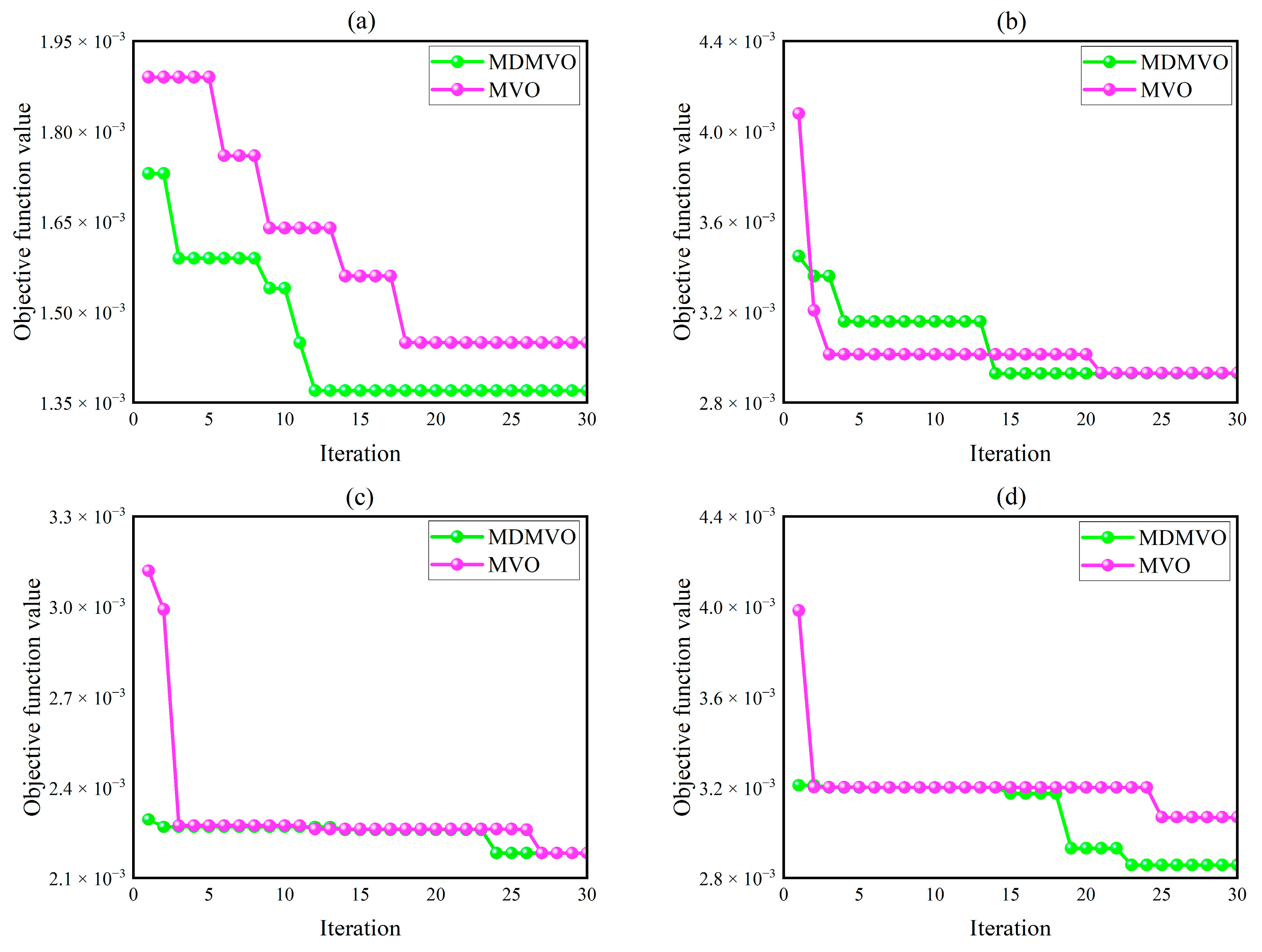
In this paper, an improved MDMVO algorithm is proposed. Through Latin hypercube sampling, nonlinear convergence factor and multiple disturbance strategies, the MVO algorithm is optimized globally. Therefore, the MDMVO algorithm obtains better optimization finding accuracy and convergence speed compared to the original MVO algorithm.

(3)

Aiming at the shortcomings of the MCKD method in fault feature extraction of rolling element bearings under a strong noise environment, a parameter-adaptive optimization MCKD fault feature extraction method is proposed. Using the MDMVO, avoiding the interference of human subjective factors on the selection of MCKD parameters and achieving the best deconvolution of fault signals.

From the perspective of reality, the CCERLMDAN proposed in this paper is affected by noise standard deviation and the number of ensembles. The fault diagnosis method proposed in this paper combines a large number of algorithms and has a certain signal processing delay, especially in the processing of the MDMVO algorithm for the selection of MCKD-adaptive parameters. In future research, we will focus on the optimal selection of noise standard deviation and the number of ensembles, and optimize the delay. In addition, in the future, we will add real engineering cases to further improve and test the effectiveness of the proposed method.

References

1. Wang, L.; Liu, Z.; Miao, Q.; Zhang, X. Complete ensemble local mean decomposition with adaptive noise and its application to fault diagnosis for rolling bearings. Mech. Syst. Signal Process. 2018, 106, 24–39. [Google Scholar] [CrossRef]
2. Wang, L.; Liu, Z. An improved local characteristic-scale decomposition to restrict end effects, mode mixing and its application to extract incipient bearing fault signal. Mech. Syst. Signal Process. 2021, 156, 107657. [Google Scholar] [CrossRef]
3. Li, J.; Li, M.; Zhang, J. Rolling bearing fault diagnosis based on time-delayed feedback monostable stochastic resonance and adaptive minimum entropy deconvolution. J. Sound Vibr. 2017, 401, 139–151. [Google Scholar] [CrossRef]
4. Peng, P.Z.; Song, Y.; Yang, L.; Wei, H.K. Seizure Prediction in EEG Signals Using STFT and Domain Adaptation. Front. Neurosci. 2022, 15, 1880. [Google Scholar] [CrossRef] [PubMed]
5. Pachori, R.B.; Nishad, A. Cross-terms reduction in the Wigner–Ville distribution using tunable-Q wavelet transform. Signal Process. 2016, 120, 288–304. [Google Scholar] [CrossRef]
6. Shao, R.; Hu, W.; Wang, Y.; Qi, X. The fault feature extraction and classification of gear using principal component analysis and kernel principal component analysis based on the wavelet packet transform. Measurement 2014, 54, 118–132. [Google Scholar] [CrossRef]
7. Hu, C.; Xing, F.; Pan, S.; Yuan, R.; Lv, Y. Fault Diagnosis of Rolling Bearings Based on Variational Mode Decomposition and Genetic Algorithm-Optimized Wavelet Threshold Denoising. Machines 2022, 10, 649. [Google Scholar] [CrossRef]
8. Huang, N.E.; Shen, Z.; Long, S.R.; Wu, M.C.; Shih, H.H.; Zheng, Q.; Yen, N.-C.; Tung, C.C.; Liu, H.H. The Empirical Mode Decomposition and the Hilbert Spectrum for Nonlinear and Non-Stationary Time Series Analysis. Proc. R. Soc. A-Math. Phys. Eng. Sci. 1998, 454, 903–995. [Google Scholar] [CrossRef]
9. Ompokov, V.D.; Boronoev, V.V. Mode Decomposition and the Hilbert-Huang Transform. In Proceedings of the 2019 Russian Open Conference on Radio Wave Propagation (RWP), Kazan, Russia, 1–6 July 2019; Volume 1, pp. 222–223. [Google Scholar]
10. Valdes, G.; O’Reilly, B.; Diaz, M. A Hilbert-Huang transform method for scattering identification in LIGO. Class. Quantum Gravity 2017, 34, 235009. [Google Scholar] [CrossRef] [Green Version]
11. Alaifari, R.; Wellershoff, M. Uniqueness of STFT phase retrieval for bandlimited functions. Appl. Comput. Harmon. Anal. 2021, 50, 34–48. [Google Scholar] [CrossRef]
12. Feng, Z.P.; Liang, M.; Chu, F.L. Recent advances in time-frequency analysis methods for machinery fault diagnosis: A review with application examples. Mech. Syst. Signal Process. 2013, 38, 165–205. [Google Scholar] [CrossRef]
13. Yang, Y.; Peng, Z.K.; Zhang, W.M.; Meng, G. Parameterised time-frequency analysis methods and their engineering applications: A review of recent advances. Mech. Syst. Signal Process. 2019, 119, 182–221. [Google Scholar] [CrossRef]
14. Kumar, K.M.A.; Manjunath, T.C. Vibration Signal Analysis using Time and Timefrequency Domain: Review. In Proceedings of the 2017 IEEE International Conference on Power, Control, Signals and Instrumentation Engineering (ICPCSI), Chennai, India, 21–22 September 2017; pp. 1808–1811. [Google Scholar]
15. Smith, J.S. The local mean decomposition and its application to EEG perception data. J. R. Soc. Interface 2005, 2, 443–454. [Google Scholar] [CrossRef] [PubMed]
16. Fan, S.S.; Wang, X.H.; Yang, S.Y. Voltage Disturbance Signals Identification Based on ILMD and Neural Network. Int. J. Pattern Recognit. Artif. Intell. 2020, 34, 2058007. [Google Scholar] [CrossRef]
17. Liang, J.H.; Wang, L.P.; Wu, J.; Liu, Z.G.; Yu, G. Elimination of end effects in LMD by Bi-LSTM regression network and applications for rolling element bearings characteristic extraction under different loading conditions. Digit. Signal Prog. 2020, 107, 102881. [Google Scholar] [CrossRef]
18. Nassef, M.G.A.; Hussein, T.M.; Mokhiamar, O. An adaptive variational mode decomposition based on sailfish optimization algorithm and Gini index for fault identification in rolling bearings. Measurement 2021, 173, 108514. [Google Scholar] [CrossRef]
19. Liu, Z.L.; Jin, Y.Q.; Zuo, M.J.; Feng, Z.P. Time-frequency representation based on robust local mean decomposition for multicomponent AM-FM signal analysis. Mech. Syst. Signal Process. 2017, 95, 468–487. [Google Scholar] [CrossRef]
20. Ma, J.; Liu, F. Bearing Fault Diagnosis with Variable Speed Based on Fractional Hierarchical Range Entropy and Hunter-Prey Optimization Algorithm-Optimized Random Forest. Machines 2022, 10, 763. [Google Scholar] [CrossRef]
21. Huynh, A.N.L.; Deo, R.C.; Ali, M.; Abdulla, S.; Raj, N. Novel short-term solar radiation hybrid model: Long short-term memory network integrated with robust local mean decomposition. Appl. Energy 2021, 298, 117193. [Google Scholar] [CrossRef]
22. Wang, Z.C.; Chen, H.Y.; Zhu, J.M.; Ding, Z.N. Daily PM2.5 and PM10 forecasting using linear and nonlinear modeling framework based on robust local mean decomposition and moving window ensemble strategy. Appl. Soft. Comput. 2022, 114, 108110. [Google Scholar] [CrossRef]
23. Xu, G.M.; Yang, Z.X.; Wang, S. Study on mode mixing problem of empirical mode decomposition. In Proceedings of the 2016 Joint International Information Technology, Mechanical and Electronic Engineering, Xi’an, China, 3–5 October 2016; Volume 59, pp. 389–394. [Google Scholar]
24. Yeh, J.R.; Shieh, J.S.; Huang, N.E. Complementary ensemble empirical mode decomposition: A novel noise enhanced data analysis method. Adv. Adapt. Data Anal. 2010, 2, 135–156. [Google Scholar] [CrossRef]
25. Colominas, M.A.; Schlotthauer, G.; Torres, M.E. Improved complete ensemble EMD: A suitable tool for biomedical signal processing. Biomed. Signal Process. Control 2014, 14, 19–29. [Google Scholar] [CrossRef]
26. Endo, H.; Randall, R.B. Enhancement of autoregressive model based gear tooth fault detection technique by the use of minimum entropy deconvolution filter. Mech. Syst. Signal Process. 2007, 21, 906–919. [Google Scholar] [CrossRef]
27. McDonald, G.L.; Zhao, Q.; Zuo, M.J. Maximum correlated Kurtosis deconvolution and application on gear tooth chip fault detection. Mech. Syst. Signal Process. 2012, 33, 237–255. [Google Scholar] [CrossRef]
28. Deng, W.; Li, Z.; Li, X.; Chen, H.; Zhao, H. Compound Fault Diagnosis Using Optimized MCKD and Sparse Representation for Rolling Bearings. IEEE Trans. Instrum. Meas. 2022, 71, 3508509. [Google Scholar] [CrossRef]
29. Tang, G.J.; Wang, X.L.; He, Y.L. Diagnosis of compound faults of rolling bearings through adaptive maximum correlated kurtosis deconvolution. J. Mech. Sci. Technol. 2016, 30, 43–54. [Google Scholar] [CrossRef]
30. Lyu, X.; Hu, Z.; Zhou, H.; Wang, Q. Application of improved MCKD method based on QGA in planetary gear compound fault diagnosis. Measurement 2019, 139, 236–248. [Google Scholar] [CrossRef]
31. Mirjalili, S.; Gandomi, A.H.; Mirjalili, S.Z.; Saremi, S.; Faris, H.; Mirjalili, S.M. Salp Swarm Algorithm: A bio-inspired optimizer for engineering design problems. Adv. Eng. Softw. 2017, 114, 163–191. [Google Scholar] [CrossRef]
32. Mirjalili, S. SCA: A Sine Cosine Algorithm for solving optimization problems. Knowl.-Based Syst. 2016, 96, 120–133. [Google Scholar] [CrossRef]
33. Mirjalili, S.; Mirjalili, S.M.; Hatamlou, A. Multi-Verse Optimizer: A nature-inspired algorithm for global optimization. Neural Comput. Appl. 2016, 27, 495–513. [Google Scholar] [CrossRef]
34. Li, X.; Bi, F.; Zhang, L.; Yang, X.; Zhang, G. An Engine Fault Detection Method Based on the Deep Echo State Network and Improved Multi-Verse Optimizer. Energies 2022, 15, 1205. [Google Scholar] [CrossRef]
35. Wei, Z.; Zhao, X. Multi-UAVs Cooperative Reconnaissance Task Allocation Under Heterogeneous Target Values. IEEE Access 2022, 10, 70955–70963. [Google Scholar] [CrossRef]
36. Zhao, X.D.; Fang, Y.M.; Liu, L.; Xu, M.; Li, Q. A covariance-based Moth-flame optimization algorithm with Cauchy mutation for solving numerical optimization problems. Appl. Soft. Comput. 2022, 119, 108538. [Google Scholar] [CrossRef]
37. Han, L.; Xu, H.S.; Ma, J.M.; Jia, Z.C. A Feature Selection Method of the Island Algorithm Based on Gaussian Mutation. Wirel. Commun. Mob. Comput. 2022, 2022, 1438999. [Google Scholar] [CrossRef]
38. Campeau, W.; Simons, A.M.; Stevens, B. The evolutionary maintenance of Levy flight foraging. PLoS Comput. Biol. 2022, 18, e1009490. [Google Scholar] [CrossRef] [PubMed]
39. Wang, J.; Liu, W.Y.; Zhang, S. An approach to eliminating end effects of EMD through mirror extension coupled with support vector machine method. Pers. Ubiquitous Comput. 2019, 23, 443–452. [Google Scholar] [CrossRef]
40. Torres, M.E.; Colominas, M.A.; Schlotthauer, G.; Flandrin, P. A complete ensemble empirical mode decomposition with adaptive noise. In Proceedings of the 2011 IEEE International Conference on Acoustics, Speech and Signal Processing (ICASSP), Prague, Czech Republic, 22–27 May 2011; pp. 4144–4147. [Google Scholar]
41. Akhenia, P.; Bhavsar, K.; Panchal, J.; Vakharia, V. Fault severity classification of ball bearing using SinGAN and deep convolutional neural network. Proc. Inst. Mech. Eng. Part C-J. Eng. Mech. Eng. Sci. 2022, 236, 3864–3877. [Google Scholar] [CrossRef]
42. Wang, B.; Lei, Y.G.; Li, N.P.; Li, N.B. A Hybrid Prognostics Approach for Estimating Remaining Useful Life of Rolling Element Bearings. IEEE Trans. Reliab. 2020, 69, 401–412. [Google Scholar] [CrossRef]
43. Antoni, J. Fast computation of the kurtogram for the detection of transient faults. Mech. Syst. Signal Process. 2007, 21, 108–124. [Google Scholar] [CrossRef]
Figure 1. Decomposition results of δ ( t ) : (a) CEEMDAN (b) ICEEMDAN and (c) CCERLMDAN. (Setting the same noise standard deviation parameter and ensemble number parameter in three methods).
Machines 10 00883 g001
Figure 2. The power spectral densities (PSD) of the modal components: (a) CEEMDAN (b) ICEEMDAN and (c) CCERLMDAN.
Machines 10 00883 g002
Figure 3. The sifting iterations obtained by (a) CEEMDAN (b) ICEEMDAN and (c) CCERLMDAN.
Machines 10 00883 g003
Figure 4. Residual noise from: (a) CEEMDAN (b) ICEEMDAN and (c) CCERLMDAN.
Machines 10 00883 g004
Figure 5. The synthesis analog signal x ( t ) and its three superimposed simulation signals x1(t), x2(t), x3(t).
Machines 10 00883 g005
Figure 6. The results of the synthesis signal decomposed by: (a) CEEMDAN, (b) ICEEMDAN, (c) RLMD, and (d) CCERLMDAN. (Setting the same noise standard deviation parameter and ensemble number parameter in three methods).
Machines 10 00883 g006
Figure 7. Residual noise from: (a) CEEMDAN, (b) ICEEMDAN, (c) RLMD, (d) CCERLMDAN.
Machines 10 00883 g007
Figure 8. (a) Comparison of methods for population initialization distribution, (b) Cauchy mutation, (c) Gaussian mutation, (d) Nonlinear convergence factor, (e) Lévy flight and (f) Schematic of the MDMVO algorithm.
Machines 10 00883 g008
Figure 9. Convergence curves of seven methods on test functions F1, F2, F3, F4, F5 and F6.
Machines 10 00883 g009
Figure 10. Wilcoxon rank-sum test for MDMVO compared with the other six techniques: (a) p - v a l u e and (b) h-value.
Machines 10 00883 g010
Figure 11. Flowchart for the approach of fault diagnostics proposed in this study.
Machines 10 00883 g011
Figure 12. (a) XJTU-SY rolling element bearing test bench, (b) the test bearing, (c) the test bearing with inner race defect, (d) the test bearing with outer race defect, and (e) the test bearing with cage defect.
Machines 10 00883 g012
Figure 13. (a) The 2100 r/min outer race fault signal and (b) its envelope spectrum.
Machines 10 00883 g013
Figure 14. The SI value for each PF was calculated by processing the outer race fault signal at 2100 r/min: (a) RLMD and (b) CCERLMDAN.
Machines 10 00883 g014
Figure 15. (a) The best PF in the RLMD envelope spectrum, and (b) The best PF in the CCERLMDAN envelope spectrum.
Machines 10 00883 g015
Figure 16. The outcomes produced by MDMVO-MCKD adaptively enhancing fault pulse: (a) The best deconvoluted signal and (b) its envelope spectrum.
Machines 10 00883 g016
Figure 17. (a) The 2400 r/min compound fault signal and (b) its envelope spectrum.
Machines 10 00883 g017
Figure 18. The SI value for each PF were calculated by processing the compound fault signal at 2400 r/min: (a) RLMD and (b) CCERLMDAN.
Machines 10 00883 g018
Figure 19. (a) The best PF in the RLMD envelope spectrum, and (b) The best PF in the CCERLMDAN envelope spectrum.
Machines 10 00883 g019
Figure 20. The outcomes produced by MDMVO-MCKD adaptively enhance the inner race fault pulse: (a) The best deconvoluted signal, and (b) its envelope spectrum.
Machines 10 00883 g020
Figure 21. The outcomes produced by MDMVO-MCKD adaptively enhance the outer race fault pulse: (a) The best deconvoluted signal, and (b) its envelope spectrum.
Machines 10 00883 g021
Figure 22. The outcomes produced by MDMVO-MCKD adaptively enhancing the roller fault pulse: (a) The best deconvoluted signal, and (b) its envelope spectrum.
Machines 10 00883 g022
Figure 23. Comparison of MCKD parameters optimized by MDMVO and MVO: (a) extraction of outer race fault, (b) inner race fault extraction from compound fault signal, (c) outer race fault extraction from compound fault signal, (d) roller fault extraction from compound fault signal.
Machines 10 00883 g023
Figure 24. Processing 2100 r/min outer race fault signal with Fast Kurtogram: (a) Kurtogram diagram, (b) Filtered signal, and (c) its square envelope spectrum.
Machines 10 00883 g024
Figure 25. (a) The filtered signal from MED by processing the selected PF in the outer race fault signal, and (b) the envelope spectrum of filtered signal.
Machines 10 00883 g025
Figure 26. Processing 2400 r/min compound fault signal with Fast Kurtogram: (a) Kurtogram diagram, (b) Filtered signal, and (c) its square envelope spectrum.
Machines 10 00883 g026
Figure 27. (a) The filtered signal from MED by processing the selected PF in the compound fault signal, and (b) the envelope spectrum of filtered signal.
Machines 10 00883 g027