An Overview of Generalized Gamma Mittag–Leffler Model and Its Applications

Abstract

Recently, probability models with thicker or thinner tails have gained more importance among statisticians and physicists because of their vast applications in random walks, L$\acute{e}$vi flights, financial modeling, etc. In this connection, we introduce here a new family of generalized probability distributions associated with the Mittag–Leffler function. This family gives an extension to the generalized gamma family, opens up a vast area of potential applications and establishes connections to the topics of fractional calculus, nonextensive statistical mechanics, Tsallis statistics, superstatistics, the Mittag–Leffler stochastic process, the L$\acute{e}$vi process and time series. Apart from examining the properties, the matrix-variate analogue and the connection to fractional calculus are also explained. By using the pathway model of Mathai, the model is further generalized. Connections to Mittag–Leffler distributions and corresponding autoregressive processes are also discussed.

1. Introduction

In model building situations in physical, biological, social and engineering sciences, the usual procedure is to select a probability model from a parametric family of distributions. In many practical problems, it is often found that the selected model is not a good fit for the experimental data, because it requires a model with a thicker or thinner tail than the ones available from the parametric family of distributions. In order to make the tail thicker or thinner, a technique is introduced here by augmenting a series to the original density. Our first step is to construct the thicker or thinner tailed distribution associated with the Mittag–Leffler function, because this function is connected to fractional calculus, the Mittag–Leffler stochastic process, non-Gaussian time series, L$\acute{e}$vi flights and in a limiting process to the topics of Tsallis statistics, superstatistics, as well as to statistical distribution theory.

In reaction rate theory, input-output type situations and reaction-diffusion problems in physics and chemistry, when the integer derivatives are replaced by fractional derivatives, the solutions automatically go in terms of Mittag–Leffler functions and their generalizations; see Haubold and Mathai (2000) [1]. The ordinary and generalized Mittag–Leffler functions interpolate between a purely exponential law and power-law-like behavior of phenomena governed by ordinary kinetic equations and their fractional counterparts; see Kilbas et al. (2004) [2], Kiryakova (2000) [3], Mathai (2010) [4] and Mathai et al. (2010) [5]. This paper examines a new family of statistical distributions associated with Mittag–Leffler functions, which gives an extension to the gamma family, which will then connect to fractional calculus and statistical distribution theory through the theory of special functions. The model investigated in this paper is useful in the study of life testing problems, reliability analysis, in physical situations to describe stable solutions, as well as unstable and chaotic neighborhoods, etc. We will start with the definition of the Mittag–Leffler function.

A two-parameter Mittag–Leffler function is defined as follows:

$$E_{\mathsf{\alpha },\mathsf{\beta }}(x^{\mathsf{\alpha }})=\sum _{k=0}^{\infty }\frac{x^{\mathsf{\alpha }k}}{\mathrm{\Gamma }(\mathsf{\alpha }k+\mathsf{\beta })},\Re (\mathsf{\alpha })>0,\Re (\mathsf{\beta })>0,$$

(1)

where $\Re (·)$ denotes the real part of $(·)$. Observe that the Mittag–Leffler function is an extension of the exponential function. When $\mathsf{\alpha }=1,\mathsf{\beta }=1$, Equation (1) reduces to ${\mathrm{e}}^x$. In statistical model building, usually, the parameters are real, but since the results to be discussed hold for complex parameters, as well, we will state the corresponding relevant conditions. Various properties, generalizations and applications of the Mittag–Leffler function can be seen from Kilbas et al. (2004) [2].

Consider a probability density of the form:

$$f(x)=\left\{\begin{array}{c}{a}^{\mathsf{\beta }}[1+\frac{\delta }{a^{\mathsf{\alpha }}}]x^{\mathsf{\beta }-1}{\mathrm{e}}^{-ax}{E}_{\mathsf{\alpha },\mathsf{\beta }}(-\delta x^{\mathsf{\alpha }}),\mathsf{\beta }>0,\mathsf{\alpha }>0,a>0,x\ge 0\hfill \\ 0,\mathrm{elsewhere},\hfill \end{array}\right.$$

(2)

where C is the normalizing constant and $E_{\mathsf{\alpha },\mathsf{\beta }}(-\mathsf{\delta }{x}^{\mathsf{\alpha }})$ is the Mittag–Leffler function. Some interesting special cases of Equation (2) are the following: The density in Equation (2) includes two-parameter gamma, exponential, chi square, noncentral chi square and the like. When $\mathsf{\delta }=0$, Equation (2) reduces to the two-parameter gamma density:

$$f_1(x)=C_1{x}^{\mathsf{\beta }-1}{\mathrm{e}}^{-ax},x\ge 0.$$

(3)

For $\mathsf{\alpha }=\mathsf{\beta }=1$ in Equation (2), we have the exponential density. For $\mathsf{\beta }=\frac{n}{2}$ and $a=\frac{1}{2}$ in $f_1(x)$, we have the chi square density with n degrees of freedom. For $\mathsf{\beta }=p,p=2,3,\cdots$ in Equation (3), we have the Erlang density. For $p=1$ in Erlang density, we have the exponential density. For fixed values of $a,\mathsf{\beta }$ and for various values of δ, we can look at the graphs that give a suitable interpretation to the model in Equation (2).

The above figures show a comparison between gamma density and gamma Mittag–Leffler density for different values of δ. Observe that $\mathsf{\delta }=0$ corresponds to the gamma density. In Figure 1, as the value of δ decreases, the right tail of the new density becomes thicker and thicker compared to that of a gamma density. Similarly the peakedness of the curve slowly decreases. In Figure 2, also, $\mathsf{\delta }=0$ corresponds to the gamma density. When the values of δ increases from $\mathsf{\delta }=0$, the right tail of the new density becomes thinner and thinner compared to that of a gamma density. Similarly, the peakedness of the curve slowly increases. Hence, when we look for a model with a thicker or thinner tail while a gamma density is found to be more or less a proper fit, then a member from the new family of densities introduced here will become quite useful and handy. Observe that the new density is mathematically and computationally easily tractable, just like a gamma density.

The moment-generating function of Equation (2) is given by:

$$\begin{array}{ccc}\hfill M_x(t)& =& a^{\mathsf{\beta }}[1+\frac{\mathsf{\delta }}{a^{\mathsf{\alpha }}}]{\int }_0^{\infty }{x}^{\mathsf{\beta }-1}{\mathrm{e}}^{-(a-t)x}\sum _0^{\infty }\frac{{(-\mathsf{\delta }{x}^{\mathsf{\alpha }})}^k}{\mathrm{\Gamma }({\mathsf{\alpha }}_k+\mathsf{\beta })}\mathrm{d}x\hfill \\ & =& a^{\mathsf{\beta }}[1+\frac{\mathsf{\delta }}{a^{\mathsf{\alpha }}}]\sum _0^{\infty }\frac{{(-\mathsf{\delta })}^k}{\mathrm{\Gamma }({\mathsf{\alpha }}_k+\mathsf{\beta })}{\int }_0^{\infty }{x}^{\mathsf{\alpha }k+\mathsf{\beta }-1}{\mathrm{e}}^{-(a-t)x}\mathrm{d}x.\hfill \end{array}$$

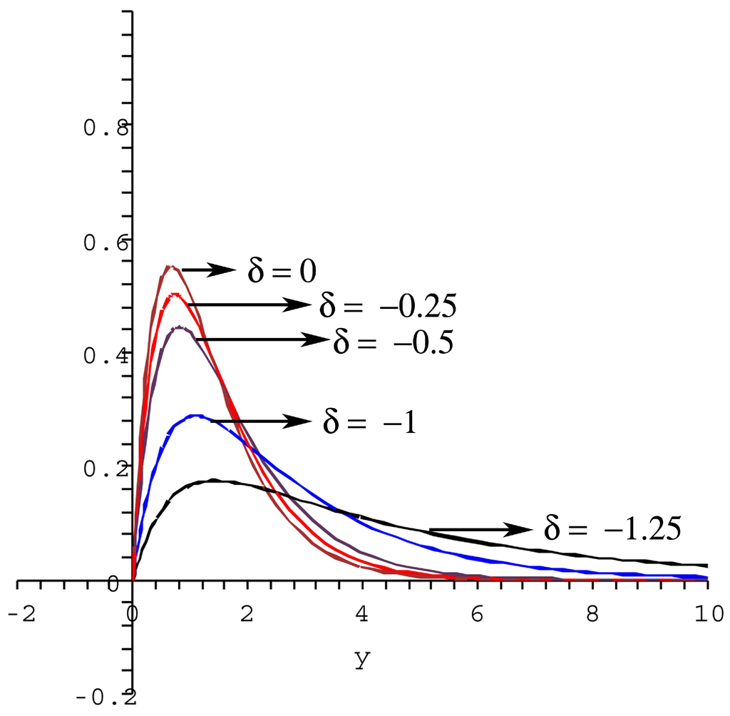
Figure 1. For $a=1.5,\mathsf{\beta }=2$ and $\mathsf{\delta }<0$.

Figure 1. For $a=1.5,\mathsf{\beta }=2$ and $\mathsf{\delta }<0$.

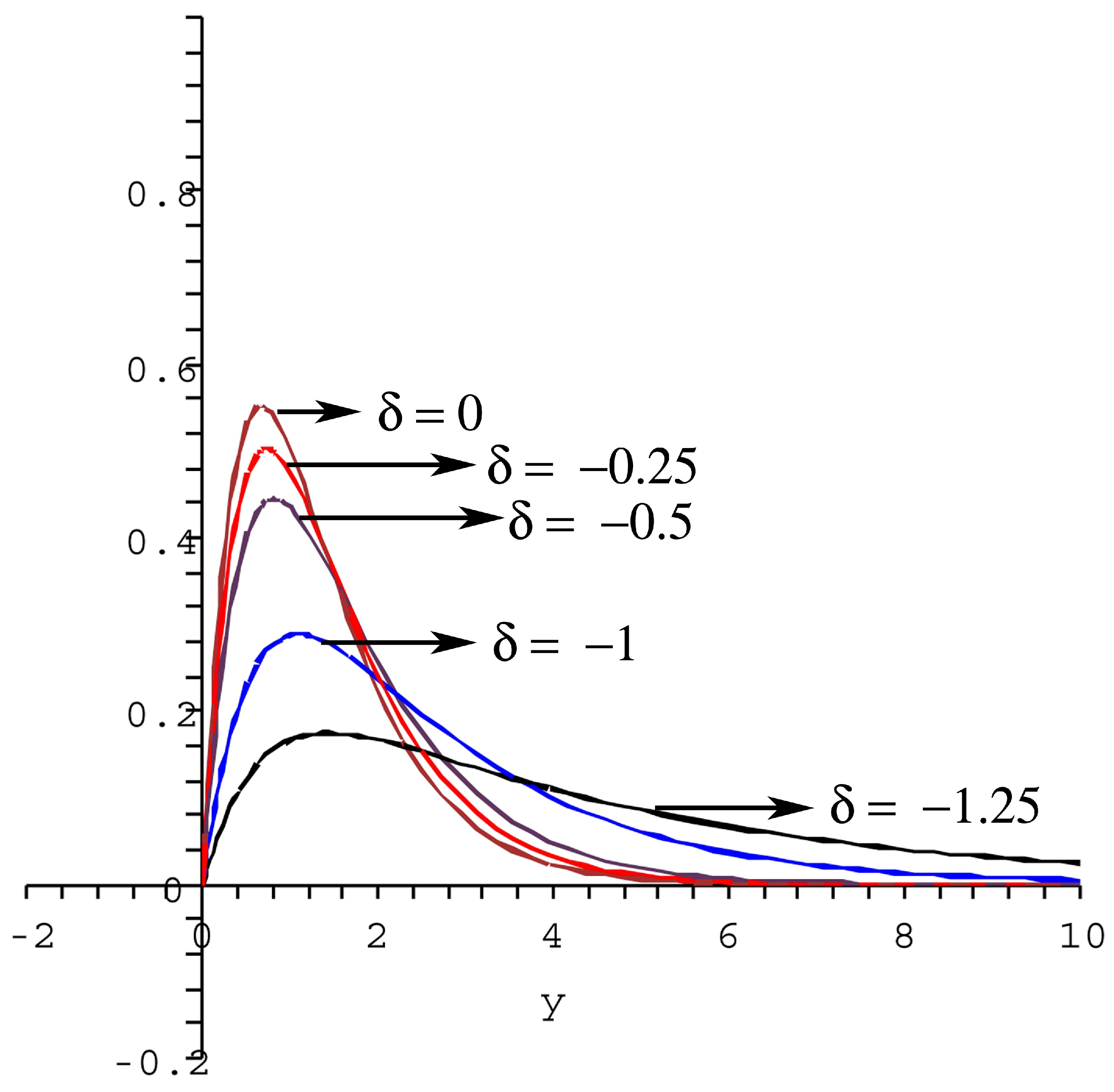
Figure 2. For $a=1.5,\mathsf{\beta }=2$ and $\mathsf{\delta }>0$.

Figure 2. For $a=1.5,\mathsf{\beta }=2$ and $\mathsf{\delta }>0$.

On simplification, we obtain mgfas:

$$M_x(t)=\frac{a^{\mathsf{\beta }}}{{(a-t)}^{\mathsf{\beta }}}\frac{(1+\frac{\mathsf{\delta }}{a^{\mathsf{\alpha }}})}{(1+\frac{\mathsf{\delta }}{{(a-t)}^{\mathsf{\alpha }}})},|\frac{\mathsf{\delta }}{{(a-t)}^{\mathsf{\alpha }}}|<1,(a-t)>0.$$

(4)

The characteristic function can be obtained if we replace t by $it,i=\sqrt{-1}$. If we put $-t$ instead of t, then we will obtain the Laplace transform of the density. Using the Laplace transform or moment-generating function, we can easily obtain the integer moments by using the following formula:

$${\mathsf{\mu }}_r^{\prime }=E(x^r)={(-1)}^r\frac{{\mathrm{d}}^r}{\mathrm{d}{t}^r}{L}_f(t){|}_{t=0}.$$

Thus, the mean value will be obtained as:

$${\mathsf{\mu }}_1^{\prime }=\frac{\mathsf{\beta }}{a}-\frac{\mathsf{\delta }\mathsf{\alpha }}{a(a^{\mathsf{\alpha }}+\mathsf{\delta })},$$

(5)

and:

$${\mathsf{\mu }}_2^{\prime }=\frac{1}{a^2}\left\{2{\mathsf{\alpha }}^2{(\frac{\mathsf{\delta }}{a^{\mathsf{\alpha }}+\mathsf{\delta }})}^2-({\mathsf{\alpha }}^2+\mathsf{\alpha }(2\mathsf{\beta }+1))(\frac{\mathsf{\delta }}{a^{\mathsf{\alpha }}+\mathsf{\delta }})+\mathsf{\beta }(\mathsf{\beta }+1)\right\}.$$

(6)

Variance:

$${\mathsf{\mu }}_2=\frac{\mathsf{\beta }}{a^2}-\frac{\mathsf{\delta }\mathsf{\alpha }[(\mathsf{\alpha }+1)a^{\mathsf{\alpha }}+\mathsf{\delta }]}{a^2{(a^{\mathsf{\alpha }}+\mathsf{\delta })}^2}.$$

Arbitrary moments can be obtained in terms of the generalized Wright hypergeometric function. That is,

$${\mathsf{\mu }}_{\gamma }^{\prime }=E(x^{\gamma })={\int }_0^{\infty }{x}^{\gamma }f(x)\mathrm{d}x$$

which is nothing but the Mellin transform of the function f with $\gamma =s-1$.

$${\mathsf{\mu }}_{\gamma }^{\prime }=\frac{(1+\frac{\mathsf{\delta }}{a^{\mathsf{\alpha }}})}{a^{\gamma }}{}_2{\Psi }_1\left[{}_{(\mathsf{\beta },\mathsf{\alpha })}^{(1,1),(\mathsf{\beta }+\gamma ,\mathsf{\alpha })}|-\frac{\mathsf{\delta }}{a^{\mathsf{\alpha }}}\right]$$

(7)

where ${}_p{\Psi }_q(z)$ is the generalized Wright’s hypergeometric function defined for $z\in C$, complex $a_i,b_j\in C$ and ${\mathsf{\alpha }}_i,{\mathsf{\beta }}_j\in {\Re }_{+}=(0,\infty ),a_i,b_j\ne 0;i=1,2,\dots ,p;j=1,2,\dots ,q$ by the series:

$${}_p{\Psi }_q(z)\equiv {}_p{\Psi }_q\left[{}_{(b_j,{\beta }_j)1,q}^{(a_i,{\alpha }_i)1,p}|z\right]=\sum _{k=0}^{\infty }\frac{\left\{{\prod }_{i=1}^p\mathrm{\Gamma }(a_i+{\alpha }_{i}k)\right\}{z}^k}{\left\{{\prod }_{j=1}^q\mathrm{\Gamma }(b_j+{\beta }_{j}k)\right\}k!}.$$

(8)

The function in Equation (8) was introduced by Wright and is called the generalized Wright’s hypergeometric function. For convergence conditions, the existence of various contours and other properties, see Wright (1940) [6] or the theory of H-function to be discussed later. If we take γ as integers in Equation (7), then we will obtain integer moments. It may be observed that the distribution function is available in terms of a series of incomplete gamma functions.

2. Estimation of Parameters

In this section, we have given explicit forms of the estimators of the parameters using the method of moments. The motivation for the method of moments comes from the fact that the sample moments are consistent estimators for the corresponding population moments. To start with, let us consider the case for $a=1,\mathsf{\beta }=1$ in Equation (2), then the model will become the Mittag–Leffler extension of the standard exponential distribution and has the density of the form:

$$g_1(x)=(1+\mathsf{\delta }){\mathrm{e}}^{-x}{E}_{\mathsf{\alpha }}(-\mathsf{\delta }{x}^{\mathsf{\alpha }}).$$

(9)

The moments can be obtained from Equations (5) and (6) with the parameter value $a=1,\mathsf{\beta }=1$.

The moment estimators of δ and α are given by:

$$\widehat{\mathsf{\alpha }}=\frac{\sum {(x_i-\overline{x})}^2-n{\overline{x}}^2}{n(\overline{x}-1)}+1,\overline{x}\ne 1$$

and:

$$\widehat{\mathsf{\delta }}=\frac{n{(\overline{x}-1)}^2}{n\overline{x}-\sum {(x_i-\overline{x})}^2},n\overline{x}-\sum {(x_i-\overline{x})}^2\ne 0.$$

Now, consider the Mittag–Leffler extension of standard gamma density. For that, we take $a=1$ in Equation (2); thus, the model has the following form:

$$g_2(x)=(1+\mathsf{\delta })x^{\mathsf{\beta }-1}{\mathrm{e}}^{-x}{E}_{\mathsf{\alpha },\mathsf{\beta }}(-\mathsf{\delta }{x}^{\mathsf{\alpha }}).$$

(10)

Using the same procedure as above, one can obtain the estimators as:

$$\widehat{\mathsf{\beta }}=\frac{\sum {(x_i-\overline{x})}^3-[\sum {(x_i-\overline{x})}^2][\sum x_i^2+n\overline{x}]+2n\overline{x}[n{\overline{x}}^3-{\overline{x}}^2]}{\sum x_i^2[4n\overline{x}-3n-3]+n{\overline{x}}^2[8n\overline{x}+13n]+n^2\overline{x}}$$

$$\widehat{\mathsf{\alpha }}=\frac{\sum {(x_i-\overline{x})}^2-n{(\overline{x}-\widehat{\beta })}^2-n\overline{x}}{n(\overline{x}-\widehat{\mathsf{\beta }})},n(\overline{x}-\widehat{\mathsf{\beta }})\ne 0$$

and:

$$\widehat{\mathsf{\delta }}=\frac{(\widehat{\mathsf{\beta }}-\overline{x})}{\widehat{\mathsf{\alpha }}+\overline{x}-\widehat{\mathsf{\beta }}}.$$

If we retain all parameters $\mathsf{\alpha },\mathsf{\beta },\mathsf{\delta }$ and a, then the analytical solution is quite difficult, but the numerical solution can be obtained by using software like MATLAB and MAPLE.

3. The Q-Analogue of Generalized Gamma Mittag–Leffler Density

In this section, a generalized density of Equation (2) is considered. Mathai (2005) [7] introduced the pathway model, where the scalar version of the pathway density is given as follows:

$$\begin{array}{ccc}\hfill f_1(x)& =& c_1{|x|}^{\mathsf{\beta }-1}{[1+a(q-1)|x|}^{\rho }{]}^{-\frac{1}{q-1}}\hfill \\ \hfill & & \text{for}a>0,\mathsf{\beta }>0,q>1,-\infty <x<\infty \hfill \end{array}$$

(11)

$\text{where}{c}_1=\frac{\rho {[a(q-1)]}^{\frac{\mathsf{\beta }}{\rho }}\mathrm{\Gamma }(\frac{1}{q-1})}{2\mathrm{\Gamma }(\frac{\beta }{\rho })\mathrm{\Gamma }(\frac{1}{q-1}-\frac{\mathsf{\beta }}{\rho })},\frac{1}{q-1}>\frac{\mathsf{\beta }}{\rho }.$

For $q<1$, writing $q-1=-(1-q)$, we have the form:

$$\begin{array}{ccc}\hfill f_2(x)& =& c_2{|x|}^{\mathsf{\beta }-1}{[1-a(1-q)|x|}^{\rho }{]}^{\frac{1}{1-q}}\hfill \\ \hfill & & \text{for}a>0,\mathsf{\beta }>0,q<1,1-{a(1-q)|x|}^{\rho }>0\hfill \end{array}$$

(12)

$\text{where}{c}_2=\frac{\rho {[a(1-q)]}^{\frac{\mathsf{\beta }}{\rho }}\mathrm{\Gamma }(\frac{1}{1-q}+\frac{\mathsf{\beta }}{\rho }+1)}{2\mathrm{\Gamma }(\frac{\mathsf{\beta }}{\rho })\mathrm{\Gamma }(\frac{1}{1-q}+1)}.$

As $q\to 1$, $f_1(x)$ and $f_2(x)$ tend to $f_3(x)$, which we refer to as the extended symmetric generalized gamma distribution, where $f_3(x)$ is given by:

$$f_3(x)=\frac{\rho a^{\frac{\beta }{\rho }}}{2\mathrm{\Gamma }(\frac{\mathsf{\beta }}{\rho })}{|x|}^{\mathsf{\beta }-1}{\mathrm{e}}^{-{a|x|}^{\rho }},-\infty <x<\infty ,a,\mathsf{\beta },\rho >0.$$

(13)

Now, generalize Equation (2) by using Equation (11). Since the normalizing constants obtained in this section are in terms of H-functions, a definition of the H-function is given here.

$$\begin{array}{ccc}\hfill H_{p,q}^{m,n}\left[z{|}_{(b_1,{\mathsf{\beta }}_1),...,(b_q,{\mathsf{\beta }}_q)}^{(a_1,{\mathsf{\alpha }}_1),...,(a_p,{\mathsf{\alpha }}_p)}\right]& =& \frac{1}{2\pi i}{\int }_L\varphi (s)z^{-s}\mathrm{d}s,\hfill \end{array}$$

(14)

where:

$$\begin{array}{ccc}\hfill \varphi (s)& =& \frac{\left\{{\prod }_{j=1}^m\mathrm{\Gamma }(b_j+{\beta }_{j}s)\right\}\left\{{\prod }_{j=1}^n\mathrm{\Gamma }(1-a_j-{\mathsf{\alpha }}_{j}s)\right\}}{\left\{{\prod }_{j=m+1}^q\mathrm{\Gamma }(1-b_j-{\mathsf{\beta }}_{j}s)\right\}\left\{{\prod }_{j=n+1}^p\mathrm{\Gamma }(a_j+{\mathsf{\alpha }}_{j}s)\right\}}\hfill \end{array}$$

where ${\mathsf{\alpha }}_j,j=1,2,...,p,{\mathsf{\beta }}_j,j=1,2,...,q$ are real positive numbers, $a_j,j=1,2,...,p$ and $b_j,j=1,2,...,q$ are complex numbers and L is a contour separating the poles of $\mathrm{\Gamma }(b_j+{\mathsf{\beta }}_{j}s),j=1,2,...,m$ from those of $\mathrm{\Gamma }(1-a_j-{\mathsf{\alpha }}_{j}s),j=1,2,...,n$. The details of convergence conditions, various properties and applications of H-function are available in Mathai et al. (2010) [5].

Consider:

$$f_4(x)=C_4{x}^{\mathsf{\beta }-1}{[1+a(q-1)x^{\rho }]}^{-\frac{1}{q-1}}{E}_{\frac{\mathsf{\alpha }}{\rho },\frac{\mathsf{\beta }}{\rho }}(-\mathsf{\delta }{x}^{\mathsf{\alpha }}),$$

(15)

$$x\ge 0,q>1,a>0,\rho >0,\mathsf{\alpha }>0,\mathsf{\beta }>0$$

where:

$$\begin{array}{c}\hfill C_4^{-1}=\frac{1}{\rho \mathrm{\Gamma }(\frac{1}{q-1})[a{(q-1)}^{\frac{\mathsf{\beta }}{\rho }}]}{H}_{1,2}^{2,1}\left[\frac{\mathsf{\delta }}{{[a(q-1)]}^{\frac{\mathsf{\alpha }}{\rho }}}{|}_{(0,1),(\frac{1}{q-1}-\frac{\mathsf{\beta }}{\rho },\frac{\mathsf{\alpha }}{\rho })}^{(0,1)}\right],q>1.\end{array}$$

(16)

The general density in Equation (15), for $q>1$, includes the Mittag–Leffler extension of Type 2 beta density and F density. If $x>0$ is replaced by $|x|,-\infty <x<\infty$, with the appropriate change in the normalizing constant, then we have the Student t density and Cauchy density as special cases, and many more. As $q\to 1$, $f_4(x)$ reduces to $f_5(x)$, where:

$$f_5(x)=C_5{x}^{\mathsf{\beta }-1}{\mathrm{e}}^{-a{x}^{\rho }}{E}_{\frac{\mathsf{\alpha }}{\rho },\frac{\mathsf{\beta }}{\rho }}(-\mathsf{\delta }{x}^{\mathsf{\alpha }}),C_5=\rho a^{\frac{\mathsf{\beta }}{\rho }}(1+\frac{\mathsf{\delta }}{a^{\frac{\mathsf{\alpha }}{\rho }}}).$$

(17)

This includes the Mittag–Leffler extension of generalized gamma, Weibull, chi-square, Maxwell–Boltzmann and related densities. If $\mathsf{\delta }=0$, Equation (17) reduces to the generalized gamma density. When $\rho =1$, Equation (17) reduces to Equation (2). In particular, if $\rho =\mathsf{\beta }$, the Mittag–Leffler extension of Weibull density is obtained,

$$f_6(x)=C_6{x}^{\beta -1}{\mathrm{e}}^{-a{x}^{\beta }}{E}_{\frac{\alpha }{\rho },1}(-\delta x^{\alpha }).$$

(18)

For $x>0$ and $q<1$, $f_4(x)$ takes the following form:

$$f_7(x)=C_7{x}^{\mathsf{\beta }-1}{[1-a(1-q)x^{\rho }]}^{\frac{1}{1-q}}{E}_{\frac{\mathsf{\alpha }}{\rho },\frac{\mathsf{\beta }}{\rho }}(-\mathsf{\delta }{x}^{\mathsf{\alpha }}),$$

(19)

$$0\le x\le \frac{1}{{[a(1-q)]}^{\frac{1}{\rho }}},a,\mathsf{\alpha },\mathsf{\beta }>0,q<1$$

where:

$$\begin{array}{c}\hfill C_7^{-1}=\frac{\mathrm{\Gamma }(1+\frac{1}{1-q})}{\rho [a{(1-q)}^{\frac{\mathsf{\beta }}{\rho }}]}{H}_{1,2}^{1,1}\left[\frac{\mathsf{\delta }}{{[a(1-q)]}^{\frac{\mathsf{\alpha }}{\rho }}}{|}_{(0,1),(-\frac{1}{1-q}-\frac{\mathsf{\beta }}{\rho },\frac{\mathsf{\alpha }}{\rho })}^{(0,1)}\right],q<1.\end{array}$$

(20)

This general density includes the Mittag–Leffler extension of Type 1 beta density, triangular density, uniform density and many more. As $q\to 1$, Equation (15) reduces to Equation (17). For $\rho =\mathsf{\beta }$, then Equations (15) and (19) will give the two forms of extended q-Weibull density as given below.

$$f_8(x)=C_8{x}^{\mathsf{\beta }-1}{[1+a(q-1)x^{\mathsf{\beta }}]}^{-\frac{1}{q-1}}{E}_{\frac{\mathsf{\alpha }}{\mathsf{\beta }},1}(-\mathsf{\delta }{x}^{\mathsf{\alpha }}),$$

(21)

$$x\ge 0,q>1,a>0,\mathsf{\alpha }>0,\mathsf{\beta }>0$$

$$f_9(x)=C_9{x}^{\mathsf{\beta }-1}{[1-a(1-q)x^{\mathsf{\beta }}]}^{\frac{1}{1-q}}{E}_{\frac{\mathsf{\alpha }}{\mathsf{\beta }},1}(-\mathsf{\delta }{x}^{\mathsf{\alpha }}),$$

(22)

$$0\le x\le \frac{1}{{[a(1-q)]}^{\frac{1}{\mathsf{\beta }}}},a,\mathsf{\alpha },\mathsf{\beta }>0,q<1$$

where the normalizing constants $C_8$ and $C_9$ are obtained from Equations (16) and (20), respectively. In particular, if $\mathsf{\delta }=0$, then $f_8(x)$ and $f_9(x)$ will coincide with q-Weibull density. In particular, for $\mathsf{\beta }=1$ and $\rho =1$, the integral of Equation (19) can be treated as the pathway fractional integral transform of the Mittag–Leffler function with appropriate transformation of the variable. More details about pathway fractional integral transform can be found in Seema Nair ((2009) [8], (2011) [9]).

The model in Equation (15) can be connected to the superstatistics of Beck and Cohen (2003) [10] and Beck (2006) [11] for $q=2,\mathsf{\delta }=0$. There is a vast literature on Beck–Cohen superstatistics in statistical mechanics with many physical interpretations; see, for example, Beck ((2010) [12], (2009) [13]). From a statistical point of view, it can be obtained as an unconditional density from Bayes’ setup, by considering generalized gamma as a conditional density with the assumption that the scale parameter a has a prior gamma density; see Nair and Kattuveettil (2010) [14]. For $\mathsf{\beta }=1,\rho =1,a=1$ and $\mathsf{\delta }=1$, we have Tsallis statistics for $q>1$ and $q<1$, respectively, from the models in Equations (15) and (19). Thus, we can make a connection to nonextensive statistical mechanics; see, for example, Tsallis ((1988) [15], (2004) [16], (2009) [17]) and Mathai et al. (2010) [5]. (It is stated that over 3000 papers have been published on this topic during the past 20 years, and over 5000 people from around the globe are working in this area).

4. Connection to Mittag–Leffler Distributions and Autoregressive Processes

Especially when $a=0$, $\mathsf{\beta }=\mathsf{\alpha }$, such that $0<\mathsf{\alpha }\le 1$ in Equation (2), we have the Mittag–Leffler density, which has the probability density function:

$$g_1(x)=\mathsf{\delta }{x}^{\mathsf{\alpha }-1}{E}_{\mathsf{\alpha },\mathsf{\alpha }}(-\mathsf{\delta }{x}^{\mathsf{\alpha }}),0<\mathsf{\alpha }\le 1,\mathsf{\delta }>0$$

(23)

and has Laplace transform $\mathsf{\delta }{(s^{\mathsf{\alpha }}+\mathsf{\delta })}^{-1}$, a special case of the general class of Laplace transforms discussed by Mathai et al. (2006) [18]. Similarly, for $a=0$ in (2) and replacing β by $\mathsf{\alpha }\gamma$ and δ by $\frac{1}{\rho }$, one can arrive at the generalized Mittag–Leffler density, which has the probability density function:

$$g(x)=\frac{x^{\mathsf{\alpha }\gamma -1}}{{\rho }^{\gamma }}{E}_{\mathsf{\alpha },\mathsf{\alpha }\gamma }^{\gamma }(-\frac{x^{\mathsf{\alpha }}}{\rho }),0<\mathsf{\alpha }<1,\gamma ,\rho >0,x\ge 0$$

(24)

where $E_{\mathsf{\alpha },\mathsf{\beta }}^{\mathsf{\delta }}(·)$ is the generalized Mittag–Leffler function defined as:

$$E_{\mathsf{\alpha },\mathsf{\beta }}^{\mathsf{\delta }}(z)=\sum _{k=0}^{\infty }\frac{{(\mathsf{\delta })}_k{z}^k}{\mathrm{\Gamma }(\mathsf{\alpha }k+\mathsf{\beta })k!},\mathsf{\alpha }>0,\mathsf{\beta }>0,\gamma >0,$$

where ${(\mathsf{\delta })}_k=\mathsf{\delta }(\mathsf{\delta }+1)(\mathsf{\delta }+2)\cdots (\mathsf{\delta }+k-1)$ and Equation (24) has the Laplace transform of the form:

$$L_g(t)={[1+\rho t^{\mathsf{\alpha }}]}^{-\gamma },|\rho t^{\mathsf{\alpha }}|<1.$$

(25)

The Laplace transform in Equation (25) is associated with infinitely-divisible and geometrically infinitely-divisible distributions, α-Laplace and Linnik distributions. The class of Laplace transforms relevant in geometrically infinitely-divisible and α-Laplace distributions is of the form $L(p)=\frac{1}{1+\eta (p)}$, where $\eta (p)$ satisfies the condition $\eta (bp)=b^{\mathsf{\alpha }}\eta (p)$ and $\eta (p)$ is a periodic function for fixed α. In Mathai (2010) [4], it is noted that there is a structural representation in terms of the positive L$\acute{e}$vi random variable by using Equation (25).

A positive L$\acute{e}$vi random variable $u>0$, with parameter α is such that the Laplace transform of the density of $u>0$ is given by ${\mathrm{e}}^{-t^{\mathsf{\alpha }}}$. That is:

$$E[{\mathrm{e}}^{-tu}]={\mathrm{e}}^{-t^{\mathsf{\alpha }}}.$$

(26)

Theorem 4.1. Let $y>0$ be a L$\acute{e}$vi random variable with Laplace transform as in (26) and $x\ge 0$ an exponential random variable with parameter δ, and let x and y be independently distributed. Then, $u=y{x}^{\frac{1}{\alpha }}$ is distributed as generalized Mittag–Leffler random variable with Laplace transform (see [4]):

$$L_u(t)={[1+\rho t^{\alpha }]}^{-\gamma }$$

Proof: For proving this result, we will make use of the following lemma of the conditional argument.

Lemma 1.1. For two random variables u and v having a joint distribution,

$$E(u)=E[E(u|v)]$$

(27)

whenever all of the expected values exist, where the inside expectation is taken in the conditional space of u given v and the outside expectation is taken in the marginal space of v.

Now, by applying Equation (27), we have the following: Let the density of u be denoted by $g(u)$. Then, the conditional Laplace transform of g, given x, is given by:

$$E[{\mathrm{e}}^{-(t{x}^{\frac{1}{\mathsf{\alpha }}})y}|x]={\mathrm{e}}^{-t^{\mathsf{\alpha }}x}.$$

(28)

However, the right side of Equation (28) is in the form of a Laplace transform of the density of x with parameter $t^{\mathsf{\alpha }}$. Hence, the expected value of the right side, with respect to x, is available by replacing the Laplace parameter t in ${[1+\rho t]}^{-\gamma }$ (the Laplace transform of a gamma density with the scale parameter ρ and shape parameter γ) by $t^{\mathsf{\alpha }}$,

$$L_g(t)={[1+\rho t^{\mathsf{\alpha }}]}^{-\gamma },\rho >0,\gamma >0$$

(29)

which establishes the result. From Equation (27), one can observe that if we consider an arbitrary random variable y with the Laplace transform of the form:

$$L_g(t)={\mathrm{e}}^{-[\varphi (t)]}$$

(30)

whenever the expected value exists, where $\varphi (t)$ is such that:

$$\varphi (t{x}^{\frac{1}{\mathsf{\alpha }}})=x\varphi (t),\underset{t\to 0}{lim}\varphi (t)=0,$$

(31)

then from Equation (28), we have:

$$E[{\mathrm{e}}^{-(t{x}^{\frac{1}{\mathsf{\alpha }}})y}|x]={\mathrm{e}}^{-x[\varphi (t)]}.$$

(32)

Now, let x be an arbitrary positive random variable having Laplace transform, denoted by $L_x(t)$ where $L_x(t)=\psi (t)$. Then, from Equations (27) and (30), we have:

$$L_g(t)=\psi (\varphi (t)).$$

In particular, when $\mathsf{\delta }=1$ in Equation (23), we have the standard Mittag–Leffler density introduced by Pillai (1990) [19]. For the properties of Mittag–Leffler distributions connected to the autoregressive process, see the papers of Pillai and Jayakumar (1995) [20] and Jayakumar (2003) [21].

4.1. Moments from Mellin–Barnes Integral Representation

It is shown in Mathai (2010) [4] that for handling problems connected to Mittag–Leffler densities, it is convenient to use the Mellin–Barnes representation of a Mittag–Leffler function and then proceed from there. The following gives the Mellin–Barnes integral representation of $g(x)$.

$$\begin{array}{ccc}\hfill g(x)& =& \frac{1}{\mathrm{\Gamma }(\gamma )}\frac{1}{2\pi i}{\int }_{c-i\infty }^{c+i\infty }\frac{\mathrm{\Gamma }(s)\mathrm{\Gamma }(\gamma -s)}{\mathrm{\Gamma }(\alpha \gamma -\alpha s)}{x}^{\mathsf{\alpha }\gamma -1}{x}^{-\mathsf{\alpha }s}\mathrm{d}s,\Re (\gamma )>0\hfill \\ & =& \frac{1}{\mathsf{\alpha }\mathrm{\Gamma }(\gamma )}\frac{1}{2\pi i}{\int }_{c-i\infty }^{c+i\infty }\frac{\mathrm{\Gamma }(\gamma -\frac{1}{\mathsf{\alpha }}+\frac{s}{\mathsf{\alpha }})\mathrm{\Gamma }(\frac{1}{\mathsf{\alpha }}-\frac{s}{\mathsf{\alpha }})}{\mathrm{\Gamma }(1-s)}{x}^{-s}\mathrm{d}s,\hfill \end{array}$$

(33)

by taking $\alpha \gamma -1-\mathsf{\alpha }s=-s_1$. One can also look upon the Mellin transform of the density of a positive random variable as the $(s-1)$-th moment, and therefore, from Equation (33), one can write the Mellin transform as an expected value. That is,

$$\begin{array}{ccc}\hfill M_g(s)& =& E(x^{s-1})\text{in}g\hfill \\ & =& \frac{1}{\mathrm{\Gamma }(\gamma )}\frac{\mathrm{\Gamma }(\gamma -\frac{1}{\mathsf{\alpha }}+\frac{s}{\mathsf{\alpha }})\mathrm{\Gamma }(\frac{1}{\mathsf{\alpha }}-\frac{s}{\mathsf{\alpha }})}{\mathsf{\alpha }\mathrm{\Gamma }(1-s)},\hfill \\ & & \text{for}1-\alpha <\Re (s)<1,0,\mathsf{\alpha }\le 1,\gamma >0\hfill \\ & =& \frac{1}{\mathrm{\Gamma }(\gamma )}\frac{\mathrm{\Gamma }(\gamma -\frac{1}{\mathsf{\alpha }}+\frac{s}{\mathsf{\alpha }})\mathrm{\Gamma }(1+\frac{1}{\mathsf{\alpha }}-\frac{s}{\mathsf{\alpha }})}{\mathrm{\Gamma }(2-s)}.\hfill \end{array}$$

(34)

If we replace $s-1$ by ρ, then one can obtain the ρ-th moment of the generalized Mittag–Leffler density as follows:

$$E(x^{\rho })=\frac{\mathrm{\Gamma }(\gamma +\frac{\rho }{\mathsf{\alpha }})\mathrm{\Gamma }(1-\frac{\rho }{\mathsf{\alpha }})}{\mathrm{\Gamma }(\gamma )\mathrm{\Gamma }(1-\rho )},-\mathsf{\alpha }<\Re (\rho )<\mathsf{\alpha }<1.$$

In particular, for $\gamma =1$, we can arrive at the ρ-th moment of the Mittag–Leffler density of Pillai (1990) [19], Pillai and Jayakumar (1995) [20]. For $\mathsf{\alpha }\to 1$, Equation (34) reduces to:

$$M_g(t)=\frac{1}{\mathrm{\Gamma }(\gamma )}\mathrm{\Gamma }(\gamma -1+s).$$

Its inverse Mellin transform is then:

$$g_1(x)=\frac{1}{\mathrm{\Gamma }(\gamma )}\frac{1}{2\pi i}{\int }_L\mathrm{\Gamma }(\gamma -1+s)x^{-s}\mathrm{d}s=\frac{1}{\mathrm{\Gamma }(\gamma )}{x}^{\gamma -1}{\mathrm{e}}^{-x},x\ge 0,\gamma >0$$

(35)

which is the one-parameter gamma density, and for $\gamma =1$, it reduces to the exponential density. Hence, the generalized Mittag–Leffler density g can be taken as an extension of a gamma density, such as the one in Equation (35), and the Mittag–Leffler density $g_1$ as an extension of exponential density for $\gamma =1$. It is shown that generalized Mittag–Leffler density $(GMLD(\mathsf{\alpha },\gamma ,\rho ))$ is infinitely and geometrically infinitely divisible for $0<\mathsf{\alpha }\le 1,0<\gamma \le 1$, and also, it belongs to the class L; see [21]. Jose et al. (2010) [22] discussed the first order autoregressive process with $GMLD(\mathsf{\alpha },\mathsf{\beta })$ marginals. In a similar manner, we shall construct a first order autoregressive process with $GMLD(\mathsf{\alpha },\gamma ,\rho )$ marginals, which will be stated as a remark.

Remark: The first order autoregressive process $X_n=a{X}_{n-1}+{\eta }_n,a\in (0,1)$ is strictly stationary Markovian with $GMLD(\mathsf{\alpha },\gamma ,\rho )$ if and only if the $\left\{{\eta }_n\right\}$ are distributed independently and identically as the γ-fold convolution of the random variable $\left\{V_n\right\}$ where:

$$V_n=\left\{\begin{array}{c}0\text{with}\text{probability}{a}^{\mathsf{\alpha }}\hfill \\ M_n\text{with}\text{probability}1-a^{\mathsf{\alpha }}\hfill \end{array}\right.$$

(36)

where $\left\{M_n\right\}$ are independently and identically distributed Mittag–Leffler random variables, provided $X_0\stackrel{d}{=}GMLD(\mathsf{\alpha },\gamma ,\rho )$ and independent of ${\eta }_n$.

5. Applications in Reaction-Diffusion Problems

We can look at the model Equation (2) in another way, as well; consider the total integral as:

$$1=C{\int }_0^{\infty }{x}^{\mathsf{\beta }-1}{\mathrm{e}}^{-ax}{E}_{\mathsf{\alpha },\mathsf{\beta }}(-\mathsf{\delta }{x}^{\mathsf{\alpha }})\mathrm{d}x,$$

(37)

which can be treated as the Laplace transform of the function $x^{\mathsf{\beta }-1}{E}_{\mathsf{\alpha },\mathsf{\beta }}(-\mathsf{\delta }{x}^{\mathsf{\alpha }})$, and hence, $C^{-1}=\frac{a^{\mathsf{\alpha }-\mathsf{\beta }}}{a^{\mathsf{\alpha }}+\mathsf{\delta }}$, where C is the normalizing constant of Equation (2), is nothing but the Laplace transform of the given function. It is shown to be very relevant in fractional reaction-diffusion problems in physics, since it naturally occurs in the derivation of the inverse Laplace transform of the functions of the type $a^{\mathsf{\alpha }}(d+b{a}^{\mathsf{\beta }})$, where a is the Laplace transform parameter and $d\mathrm{and}\mathrm{b}$ are constants.

For more details, see the papers of [8,18,23]. Reaction-diffusion equations are modeling tools for the dynamics presented by a competition between two or more species, activators and inhibitors or production and destruction, that diffuse in a physical medium. As an example, [1] considered the evolution of a star like the Sun, which is governed by a second order system of differential equations, the kinetic equations, describing the rate of change of chemical composition of the star for each species in terms of the reaction rates for destruction and production of that species [24,25,26]. Methods for modeling processes of destruction and production have been developed for bio-chemical reactions and their unstable equilibrium states [27] and for chemical reaction networks with unstable states, oscillations and hysteresis [28].

Consider an arbitrary reaction characterized by a time-dependent quantity $N=N(t)$. It is possible to equate the rate of change $\frac{\mathrm{d}N}{\mathrm{d}t}$ to a balance between the destruction rate d and the production rate p of N, that is $\frac{\mathrm{d}N}{\mathrm{d}t}=-d+p$. In general, through feedback or other interaction mechanisms, destruction and production depend on the quantity N itself: $d=\mathrm{d}(N)$ or $p=p(N)$. This dependence is complicated, since the destruction or production at time t depends not only on $N(t)$, but also on the past history $N(\tau ),\tau <t$, of the variable N. This may be formally represented by:

$$\frac{\mathrm{d}N}{\mathrm{d}t}=-d(N_i)+p(N_i)$$

(38)

where $N_i$ denotes the function defined by $N_i(t^{*})=N(t-t^{*}),t^{*}>0$. The production and destruction of species is described by kinetic equations governing the change of the number density $N_i$ of species i over time, that is,

$$\frac{\mathrm{d}{N}_i}{\mathrm{d}t}=-\sum _j{N}_i{N}_j<\sigma \nu {>}_{ij}+\sum _{k,l\ne i}{N}_k{N}_l<\sigma \nu {>}_{kl},$$

(39)

where $<\sigma \nu {>}_{mn}$ denotes the reaction probability for an interaction involving species mand n, and the summation is taken over all reactions, which either produce or destroy the species i [29]. The first sum in Equation (39) can also be written as:

$$-\sum _j{N}_i{N}_j<\sigma \nu {>}_{ij}=-N_i(\sum _j{N}_j<\sigma \nu {>}_{ij})=N_i{a}_i,$$

(40)

where $a_i$ is the statistically expected number of reactions per unit volume per unit time destroying the species i. It is also a measure of the speed at which the reaction proceeds. In the following, we are assuming that there are $N_j(j=1,\dots i,\dots )$ species j per unit volume and that for a fixed $N_i$, the number of other reacting species that interact with the i-th species is constant in a unit volume. Following the same argument, for the second sum in Equation (39) accordingly,

$$+\sum _{k,l\ne i}{N}_k{N}_l<\sigma \nu {>}_{kl}=+N_i{b}_i,$$

(41)

where $N_i{b}_i$ is the statistically expected number of the i-th species produced per unit volume per unit time for a fixed $N_i$. Note that the number density of species i, $N_i=N_i(t)$, is a function of time, while the $<\sigma \nu {>}_{mn}$, containing the thermonuclear functions (see Haubold and Kumar (2008) [30]), are assumed to depend only on the temperature of the gas, but not on the time t and number densities $N_i$. Then, Equation (38) implies that:

$$\frac{\mathrm{d}{N}_i(t)}{\mathrm{d}t}=-(a_i-b_i)N_i(t).$$

(42)

For Equation (42), we have three distinct cases, $c_i=a_i-b_i>0$, $c_i<0$ and $c_i=0$, of which the last case says that $N_i$ does not vary over time, which means that the forward and reverse reactions involving species i are in equilibrium; such a value for $N_i$ is called a fixed point and corresponds to a steady-state behavior. The first two cases exhibit that either the destruction $(c_i>0)$ of species i or production $(c_i<0)$ of species i dominates.

For the case $c_i>0$, we have:

$$\frac{\mathrm{d}{N}_i(t)}{\mathrm{d}t}=-c_i{N}_i(t),$$

(43)

with the initial condition that $N_i(t=0)=N_0$ is the number density of species i at time $t=0$, and it follows that:

$$N_i(t)\mathrm{d}t=N_0{\mathrm{e}}^{-c_{i}t}\mathrm{d}t.$$

(44)

The exponential function in Equation (44) represents the solution of the linear one-dimensional differential Equation (43) in which the rate of destruction of the variable is proportional to the value of the variable. Equation (43) does not exhibit instabilities, oscillations or chaotic dynamics, in striking contrast to its cousin, the logistic finite-difference equation [26,29]. A thorough discussion of Equation (43) and its standard solution in Equation (44) is given in [25].

Let us consider the standard fractional kinetic equation:

$$N(t)-N_0=-c^{\nu }{}_0{D}_t^{-\nu }N(t),\nu >0$$

(45)

which is derived by [1]. ${}_0{D}_t^{-\nu }$ is the Riemann–Liouville fractional integral of order ν. It is very easy to find the solution of this equation. On applying Laplace transforms on both sides, with parameter p, one has:

$$\begin{array}{ccc}\hfill L\left\{N(t)\right\}-N_{0}L\left\{1\right\}& =& -c^{\nu }L{\{}_0{D}_t^{-\nu }N(t)\}\hfill \\ \hfill L\left\{N(t)\right\}-\frac{N_0}{p}& =& -c^{\nu }{p}^{-\nu }L\left\{N(t)\right\}\hfill \\ \hfill (1+c^{\nu }{p}^{-\nu })L\left\{N(t)\right\}& =& \frac{N_0}{p}\hfill \\ \hfill L\{N(t)\}& =& \frac{N_0}{p[1+{(\frac{p}{c})}^{-\nu }]}=N_0\left[\sum _{k=0}^{\infty }{(-1)}^k{c}^{\nu k}{p}^{-(\nu k+1)}\right].\hfill \end{array}$$

Now, applying inverse Laplace transform,

$$\begin{array}{ccc}\hfill N(t)& =& N_0\sum _{k=0}^{\infty }{(-1)}^k{c}^{\nu k}{L}^{-1}\left\{p^{-(\nu k+1)}\right\}=N_0\sum _{k=0}^{\infty }{(-1)}^k\frac{{(ct)}^{\nu k}}{\mathrm{\Gamma }(\nu k+1)}.\hfill \end{array}$$

This solution can be written in terms of the Mittag–Leffler function as:

$$N(t)=N_0{E}_{\nu }(-c^{\nu }{t}^{\nu }),\nu >0.$$

(46)

Theorem 5.1. For $\nu >0$, let the coefficient of $N_0$ of the fractional integral equation be g(t) an arbitrary function, so that the fractional integral becomes:

$$N(t)-N_{0}g(t)=-c^{\nu }{}_0{D}_t^{-\nu }N(t).$$

(47)

Then, the Laplace transforms of the fractional integral equation will be:

$$L\left\{N(t)\right\}=\frac{N_{0}G(p)}{1+{(\frac{c}{p})}^{\nu }},\text{where}G(p)=L\left\{g(t)\right\}$$

(48)

Now, one can take various forms for $G(p)$; all of the special cases are considered in [23,31]. For example:

Let us consider $G(p)=p^{-\mathsf{\beta }}{}_1{F}_1({\gamma }_1,{\mathsf{\beta }}_1,p^{-\mathsf{\alpha }})$ for $\mathsf{\alpha }>0,\mathsf{\beta }>0,\nu >0,c>0$, then Equation (47) becomes:

$$\begin{array}{ccc}\hfill L\{N(t)\}& =& N_0{p}^{-\mathsf{\beta }}\frac{{\sum }_{k=0}^{\infty }\frac{{({\gamma }_1)}_k}{{({\mathsf{\beta }}_1)}_k}\frac{p^{-\mathsf{\alpha }k}}{k!}}{\left[1+{(\frac{c}{p})}^{\nu }\right]}\hfill \\ & =& N_0{p}^{-\mathsf{\beta }}\sum _{k=0}^{\infty }\frac{{({\gamma }_1)}_k}{{({\mathsf{\beta }}_1)}_k}\frac{p^{-\mathsf{\alpha }k}}{k!}\sum _{n=0}^{\infty }{(-1)}^n{(\frac{c}{p})}^{\nu n}\hfill \\ & =& N_0\sum _{k=0}^{\infty }\frac{{({\gamma }_1)}_k}{{({\mathsf{\beta }}_1)}_{k}k!}\sum _{n=0}^{\infty }{(-1)}^n{c}^{\nu n}{p}^{-(\nu n+\mathsf{\alpha }k+\mathsf{\beta })}\hfill \end{array}$$

(49)

On applying inverse Laplace transform, we get:

$$\begin{array}{ccc}\hfill N(t)& =& N_0\sum _{k=0}^{\infty }\frac{{({\gamma }_1)}_k}{{({\mathsf{\beta }}_1)}_{k}k!}\sum _{n=0}^{\infty }{(-1)}^n{c}^{\nu n}\frac{t^{\nu n+\mathsf{\alpha }k+\mathsf{\beta }-1}}{\mathrm{\Gamma }(\nu n+\mathsf{\alpha }k+\mathsf{\beta })}\hfill \\ & =& N_0{t}^{\mathsf{\beta }-1}\sum _{k=0}^{\infty }\frac{{({\gamma }_1)}_k}{{({\mathsf{\beta }}_1)}_{k}k!}{t}^{\mathsf{\alpha }k}{E}_{\nu ,\mathsf{\alpha }k+\mathsf{\beta }}(-c^{\nu }{t}^{\nu })\hfill \end{array}$$

(50)

Haubold and Mathai (2000) [1] generalized the standard kinetic Equation (43) to a standard fractional kinetic Equation (45), derived solutions of a fractional kinetic equation that contains the particle reaction rate (or thermonuclear function) as a time constant and provided the analytic technique to further investigate possible modifications of the reaction rate through a kinetic equation. The Riemann–Liouville operator in the fractional kinetic equation introduces a convolution integral with a slowly-decaying power-law kernel, which is typical for memory effects referred to in [32]. This technique may open an avenue to accommodate changes in standard solar model core physics as proposed by [33]. In the solution of the standard fractional kinetic Equation (45), given in Equation (46), the standard exponential decay is recovered for $\nu =1$. However, the Equation (46), for $0<\nu <1$, shows a power-law behavior for $t\to \infty$ and is constant (initial value $N_0$) for $t\to 0$.

6. Application in Financial Modeling

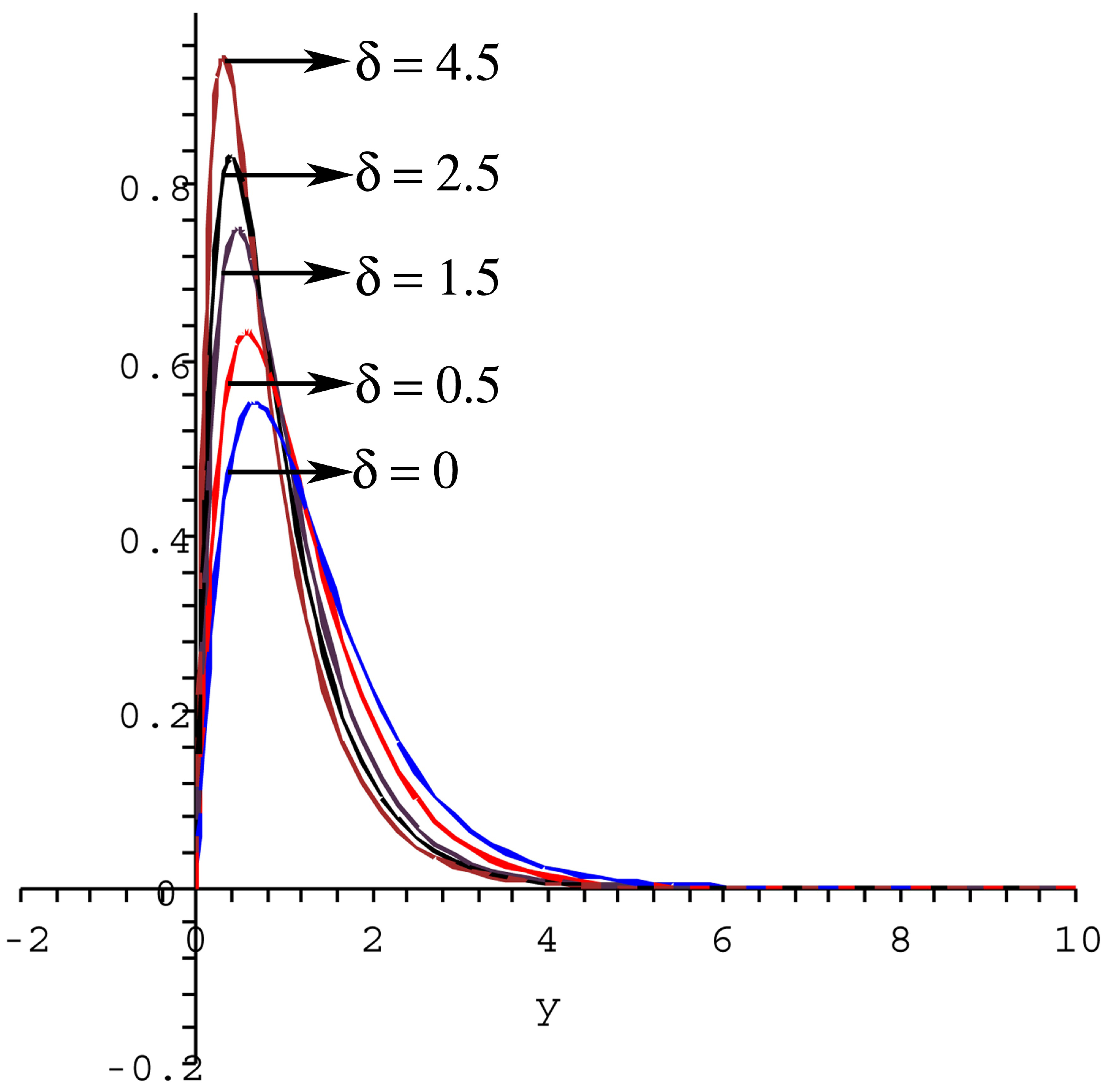
In this section, we present an application of generalized gamma Mittag–Leffler density in modeling currency exchange rates. Here, we considered 1152 observations starting from 2004 to 2008, of U.S. dollar-Indian rupee foreign exchange rates, which is available at www.rbi.org. The log returns of the exchange rates are considered. The following Figure 3 is the graph of the log-transformed data embedded with the generalized gamma Mittag–Leffler density.

From the data, the summary statistics for transformed currency exchange rates obtained are as follows:

$$\begin{array}{ccc}\hfill \mathrm{Mean}& =& 0.0110\hfill \\ \hfill \mathrm{Variance}& =& 2.0805\times {10}^{-6}\hfill \\ \hfill \mathrm{Coefficient}\mathrm{of}\mathrm{skewness}& =& 0.2728\hfill \end{array}$$

For convenience, assume that $\alpha =1$; by using the method of moments, estimates of parameters are obtained and are given as:

$$\begin{array}{ccc}\hfill \widehat{\beta }& =& 76.3057\hfill \\ \hfill \widehat{\delta }& =& 6227.6449\hfill \\ \hfill \widehat{a}& =& 7413.998\hfill \end{array}$$

From the figures, we can observe that the generalized gamma Mittag–Leffler density fits well to the data with the above estimated values of the parameters. Here, we used the chi square statistic to measure the goodness of fit. The calculated chi square value is 2.44, and the corresponding tabled value is 15.507. Hence, we conclude that the model in Equation (2) is a good fit to the dataset considered.

Figure 3. Generalized gamma Mittag–Leffler density fitted to the data on dollar-rupee exchange rate.

Figure 3. Generalized gamma Mittag–Leffler density fitted to the data on dollar-rupee exchange rate.

7. Multivariate Generalization

In this section, a multivariate analogue of the density in Equation (2) is considered. The multivariate Mittag–Leffler function will be defined as:

$$\begin{array}{ccc}\hfill & & E_p[{\mathsf{\alpha }}_1,\cdots ,{\mathsf{\alpha }}_p;{\mathsf{\beta }}_1,\cdots ,{\mathsf{\beta }}_p;-\mathsf{\delta };x_1^{{\mathsf{\alpha }}_1}\cdots x_p^{{\mathsf{\alpha }}_p}]=\sum _{k=0}^{\infty }\frac{x_1^{{\mathsf{\alpha }}_{1}k}\cdots x_p^{{\mathsf{\alpha }}_{p}k}{(-\mathsf{\delta })}^k}{\mathrm{\Gamma }({\mathsf{\alpha }}_{1}k+{\mathsf{\beta }}_1)\cdots \mathrm{\Gamma }({\mathsf{\alpha }}_{p}k+{\mathsf{\beta }}_p)},\hfill \\ & & \text{where}\Re ({\mathsf{\alpha }}_j)>0,\Re ({\mathsf{\beta }}_j>0),j=1,2,\dots ,p.\hfill \end{array}$$

(51)

A function close to $E_p(·)$ of Equation (51) is the multi-index Mittag–Leffler function of Kiryakova; see, for example, Kiryakova (2000) [3]. Now, the general density is defined as:

$$f_p(x_1,\dots ,x_p)=\left\{\begin{array}{c}{C}_p{x}_1^{{\mathsf{\beta }}_1-1}\cdots x_p^{{\mathsf{\beta }}_p-1}{\mathrm{e}}^{-a_1{x}_1-\cdots -a_p{x}_p}{E}_p[{\mathsf{\alpha }}_1,\cdots ,{\mathsf{\alpha }}_p;{\mathsf{\beta }}_1,\cdots ,{\mathsf{\beta }}_p;-\mathsf{\delta };x_1^{{\mathsf{\alpha }}_1}\cdots x_p^{{\mathsf{\alpha }}_p}],\hfill \\ 0\le x_j<\infty ,\Re ({\mathsf{\alpha }}_j)>0,\Re ({\mathsf{\beta }}_j>0),a_j>0,j=1,2,\dots ,p\hfill \\ 0,\text{elsewhere}.\hfill \end{array}\right.$$

The normalizing constant is available, by proceeding as before, as:

$$\begin{array}{ccc}\hfill C_p& =& a_1^{{\mathsf{\beta }}_1}\cdots a_p^{{\mathsf{\beta }}_p}(1+\frac{\mathsf{\delta }}{a_1^{{\mathsf{\alpha }}_1}\cdots a_p^{{\mathsf{\alpha }}_p}}),|\frac{\mathsf{\delta }}{a_1^{{\mathsf{\alpha }}_1}\cdots a_p^{{\mathsf{\alpha }}_p}}|<1.\hfill \end{array}$$

(52)

Various properties of one form of a multivariate gamma density can be seen from Griffiths (1984) [34]. The following sections reveal the joint Laplace transform and product moments of the density function.

The Joint Laplace transform is available from Equation (52) by replacing $a_j$ by $a_j+t_j,j=1,\dots ,p$ and then dividing by the normalizing constant. That is:

$$\begin{array}{ccc}\hfill E({\mathrm{e}}^{-t_1{x}_1}\cdots {\mathrm{e}}^{-t_p{x}_p})& =& \frac{a_1^{{\mathsf{\beta }}_1}\cdots a_p^{{\mathsf{\beta }}_p}}{{(a_1+t_1)}^{{\mathsf{\beta }}_1}\cdots {(a_p+t_p)}^{{\mathsf{\beta }}_p}}\frac{(1+\frac{\mathsf{\delta }}{a_1^{{\mathsf{\alpha }}_1}\cdots a_p^{{\mathsf{\alpha }}_p}})}{(1+\frac{\mathsf{\delta }}{{(a_1+t_1)}^{{\mathsf{\alpha }}_1}\cdots {(a_p+t_p)}^{{\mathsf{\alpha }}_p}})},a_j+t_j>0,\hfill \\ & & |\frac{\mathsf{\delta }}{{(a_1+t_1)}^{{\mathsf{\alpha }}_1}\cdots {(a_p+t_p)}^{{\mathsf{\alpha }}_p}}|<1,j=1,\dots ,p.\hfill \end{array}$$

(53)

The arbitrary product moments are obtained in terms of generalized Wright function and are given by:

$$\begin{array}{ccc}\hfill E(x_1^{{\gamma }_1}\cdots x_p^{{}_p})& =& {\int }_0^{\infty }\cdots {\int }_0^{\infty }{x}_1^{{\gamma }_1}\cdots x_p^{{\gamma }_p}{C}_p{x}_1^{{\mathsf{\beta }}_1-1}\cdots x_p^{{\beta }_p-1}{\mathrm{e}}^{-a_1{x}_1}\cdots {\mathrm{e}}^{-a_p{x}_p}\hfill \\ & & \times E_p({\mathsf{\alpha }}_j;{\mathsf{\beta }}_j,j=1,\dots ,p;-\mathsf{\delta };x_1^{{\mathsf{\alpha }}_1}\cdots x_p^{{\mathsf{\alpha }}_p})\mathrm{d}{x}_1\cdots \mathrm{d}{x}_p\hfill \\ & =& \frac{1}{a_1^{{\gamma }_1}\cdots a_p^{{\gamma }_p}}(1+\frac{\mathsf{\delta }}{a_1^{{\mathsf{\alpha }}_1}\cdots a_p^{{\mathsf{\alpha }}_p}}){}_{p+1}{\Psi }_p\left[{}_{({\mathsf{\beta }}_1,{\mathsf{\alpha }}_1),,({\mathsf{\beta }}_p,{\mathsf{\alpha }}_p)}^{({\mathsf{\beta }}_1+{\gamma }_1,{\mathsf{\alpha }}_1),\cdots ,({\mathsf{\beta }}_p+{\gamma }_p,{\mathsf{\alpha }}_p),(1,1)};-\frac{\mathsf{\delta }}{a_1^{{\mathsf{\alpha }}_1}\cdots a_p^{{\mathsf{\alpha }}_p}}\right],\hfill \\ & & \Re ({\mathsf{\beta }}_j+{\gamma }_j)>0,j=1,\dots ,p.\hfill \end{array}$$

(54)

Conditional density of $x_1$ given $x_2,\dots ,x_p$ is given by:

$$f(x_1|x_2,\dots ,x_p)=a_1^{{\beta }_1}{x}_1^{{\beta }_1-1}{\mathrm{e}}^{-a_1{x}_1}\frac{E_p({\alpha }_j;{\beta }_j,j=1,\dots ,p;-\delta ;x_1^{{\alpha }_1}\cdots x_p^{{\alpha }_p})}{E_{p-1}({\alpha }_j;{\beta }_j,j=2,\dots ,p;-\frac{\delta }{a_1^{{\alpha }_1}};x_2^{{\alpha }_2}\cdots x_p^{{\alpha }_p})}.$$

(55)

Regression analysis is concerned with constructing the best predictor of one variable at the preassigned values of some other variables. Under the minimum mean square principle, the best predictors can be seen to be the conditional expectation of $x_1$ given $x_2,\cdots ,x_p$. Hence, $E(x_1|x_2,\cdots ,x_p)$ is defined as the regression of $x_1$ on $x_2,\cdots ,x_p$. In our case:

$$\begin{array}{ccc}\hfill E(x_1|x_2,\dots ,x_p)& =& {\int }_0^{\infty }{x}_{1}f(x_1|x_2,\dots ,x_p)\mathrm{d}{x}_1\hfill \\ & =& \frac{1}{K(X)}{a}_1^{{\mathsf{\beta }}_1}{\int }_0^{\infty }{x}_1^{{\mathsf{\beta }}_1}{\mathrm{e}}^{-a_1{x}_1}\sum _{k=0}^{\infty }\frac{{(-\mathsf{\delta })}^k{x}_1^{{\mathsf{\alpha }}_{1}k}\cdots x_p^{{\mathsf{\alpha }}_{p}k}}{\mathrm{\Gamma }({\mathsf{\alpha }}_{1}k+{\mathsf{\beta }}_1)\cdots \mathrm{\Gamma }({\mathsf{\alpha }}_{p}k+{\mathsf{\beta }}_p)}\hfill \\ \hfill \text{where}K(X)& =& E_{p-1}({\mathsf{\alpha }}_j;{\mathsf{\beta }}_j,j=2,\dots ,p;-\frac{\mathsf{\delta }}{a_1^{{\mathsf{\alpha }}_1}};x_2^{{\mathsf{\alpha }}_2}\cdots x_p^{{\mathsf{\alpha }}_p})\hfill \end{array}$$

$$E(x_1|x_2,\dots ,x_p)=\frac{{\mathsf{\beta }}_1}{a_1}-\frac{\mathsf{\delta }{\mathsf{\alpha }}_1{x}_2^{{\mathsf{\alpha }}_2}\cdots x_p^{{\mathsf{\alpha }}_p}}{a_1^{{\mathsf{\alpha }}_1+1}}\frac{E_{p-1}^{(2)}({\mathsf{\alpha }}_j;{\mathsf{\beta }}_j+{\mathsf{\alpha }}_j,j=2,\dots ,p;-\frac{\mathsf{\delta }}{a_1^{{\mathsf{\alpha }}_1}};x_2^{{\mathsf{\alpha }}_2}\cdots x_p^{{\mathsf{\alpha }}_p})}{E_{p-1}({\mathsf{\alpha }}_j;{\mathsf{\beta }}_j,j=2,\dots ,p;-\frac{\mathsf{\delta }}{a_1^{{\mathsf{\alpha }}_1}};x_2^{{\mathsf{\alpha }}_2}\cdots x_p^{{\mathsf{\alpha }}_p})},$$

(56)

where $E_{p-1}^{(2)}$ is the same function appearing in Equation (51), but with an additional Pochhammer symbol ${(2)}_k$ sitting in the numerator. The conditional expectation, $E(x_1|x_2)$, is the best predictor, best in the sense of minimizing the expected squared error, also known as the regression of $x_1$ on $x_2$, and is given as:

$$E(x_1|x_2)=\frac{{\mathsf{\beta }}_1}{a_1}-\frac{\mathsf{\delta }{\mathsf{\alpha }}_1{x}_2^{{\mathsf{\alpha }}_2}}{a_1^{{\mathsf{\alpha }}_1+1}{a}_3^{{\mathsf{\alpha }}_3}\cdots a_p^{{\mathsf{\alpha }}_p}}\frac{E_1^{(2)}({\mathsf{\alpha }}_2;{\mathsf{\beta }}_2+{\mathsf{\alpha }}_2;-\frac{\mathsf{\delta }}{a_1^{{\mathsf{\alpha }}_1}{a}_3^{{\mathsf{\alpha }}_3}\cdots a_p^{{\mathsf{\alpha }}_p}};x_2^{{\mathsf{\alpha }}_2})}{E_1({\mathsf{\alpha }}_2;{\mathsf{\beta }}_2;-\frac{\mathsf{\delta }}{a_1^{{\mathsf{\alpha }}_1}{a}_3^{{\mathsf{\alpha }}_3}\cdots a_p^{{\mathsf{\alpha }}_p}};x_2^{{\mathsf{\alpha }}_2})}.$$

(57)

In a similar manner, we can extend the results in Section 2 to matrix-variate cases, as well. Let $X=(x_{rs})$ be $m\times n$, where all $x_{rs}$’s are distinct, X of full rank and having a joint density $f(X)$, where $f(X)$ is a real-valued scalar function of X. Then, the characteristic function of $f(X)$, denoted by ${\varphi }_X(T)$, is given by:

$${\varphi }_X(T)=E[{\mathrm{e}}^{i\text{tr}(XT)}],i=\sqrt{-1}\text{and}T=(t_{rs})$$

(58)

is an $m\times n$ matrix of distinct parameters $t_{rs}$’s, and let T be of full rank. As an example, we can look at the real matrix-variate Gaussian distribution, given by the density geometric:

$$g(X)=\frac{{|A|}^{\frac{n}{2}}{|B|}^{\frac{m}{2}}}{{\pi }^{\frac{mn}{2}}}{\mathrm{e}}^{-\text{tr}(AXB{X}^{\prime })}$$

(59)

where X is $m\times n$, $A=A^{\prime }>0$, $B=B^{\prime }>0$ are $m\times m$ and $n\times n$ positive definite constant matrices, having Fourier transform as:

$${\varphi }_g(T)={\mathrm{e}}^{-\frac{1}{4}\text{tr}(B^{-\frac{1}{2}}T{A}^{-1}{T}^{\prime }{B}^{-\frac{1}{2}})}$$

(60)

where T is the parameter matrix. Motivated by Equations (58) and (60), Mathai (2010) [4] defined matrix-variate Linnik density and gamma-Linnik density. The following result was given recently in Mathai (2010) [4], which will be needed for the discussion to follow.

Theorem 7.1. Let y be a real scalar random variable, distributed independently of the $m\times n$ matrix X and having a gamma density with the Laplace transform:

$$L_y(t)={(1+\rho t)}^{-\gamma },\rho >0,\gamma >0$$

and let X be distributed as a real rectangular matrix-variate Linnik variable having characteristic function ${\mathrm{e}}^{-{[tr(T{\Sigma }_1{T}^{\prime }{\Sigma }_2)]}^{\frac{\alpha }{2}}},0<\alpha \le 2$; then, the rectangular matrix $U=y^{\frac{1}{\alpha }}X$ has the characteristic function:

$${\varphi }_U(T)={[1+\rho {(tr(T{\Sigma }_1{T}^{\prime }{\Sigma }_2))}^{\frac{\alpha }{2}}]}^{-\beta }$$

(61)

The matrix variable U in Equation (61) will be called a real rectangular matrix-variate Gaussian Linnik variable when $\mathsf{\alpha }=2$ and gamma Linnik variable for the general α. By using the multi-index Mittag–Leffler function of Kiryakova (2000) [3] in Equation (51), one can also define a gamma-Kiryakova vector or matrix variable. Now, let us consider two independently-distributed real random variables y and X where y has a general Mittag–Leffler density as in Equation (24) and X has a real rectangular matrix-variate Gaussian density as in Equation (59). Then, we have the following results.

Theorem 7.2. Let y follow $GMLD(\mathsf{\alpha },\gamma ,\rho )$ and the real rectangular matrix X have the density in Equation (59), and let X and y be independently distributed. Then, $U_1=y^{\frac{1}{\mathsf{\alpha }}}X$ has the characteristic function:

$${\varphi }_{U_1}(T)={[1+\frac{\rho }{4^{\mathsf{\alpha }}}{(tr(A^{-1}{T}^{\prime }{B}^{-1}T))}^{\mathsf{\alpha }}]}^{-\gamma }$$

(62)

Theorem 7.3. Let $U_2=y^{\frac{1}{\mathsf{\beta }}}X$, where y and X are independently distributed with y having the density in Equation (24), and X is a real rectangular matrix-variate Linnik variable with the parameters $\gamma ,A,B$; then $U_2$ has the characteristic function:

$${\varphi }_{U_2}(T)={[1+\rho (tr{(A^{-1}{T}^{\prime }{B}^{-1}T)}^{\frac{\alpha \beta }{2}})]}^{-\gamma },\rho ,\gamma ,\alpha ,\beta >0$$

(63)

8. Conclusion

The model introduced in this paper will be useful for investigators in disciplines of physical sciences, particularly superstatistics of Beck ((2006) [11], (2009) [13]), nonextensive statistical mechanics Tsallis ((1988) [15], (2004) [16], (2009) [17]), reaction-diffusion problems in physics and Haubold (2000) [5], statistical distribution theory and model building. In many physical situations, when the integer derivatives are replaced by fractional derivatives, naturally, the solutions are obtained in terms of Mittag–Leffler functions and their generalizations. However, fractional integrals are shown to be connected to Laplace convolutions of positive random variables. Thus, one can connect the ideas of fractional calculus to statistical distribution theory via the Mittag–Leffler function. the Mittag–Leffler distribution can also be used as waiting time distributions, as well as first passage time distributions for certain renewal process.

References

- Haubold, H.J.; Mathai, A.M. The fractional kinetic equation and thermonuclear functions. Astrophys. Space Sci. 2000, 273, 53–63. [Google Scholar] [CrossRef]
- Kilbas, A.A.; Saigo, M.; Saxena, R.K. Generalized Mittag–Leffler function and generalized fractional calculus operators. J. Integral Transforms Spec. Funct. 2004, 15, 31–49. [Google Scholar] [CrossRef]
- Kiryakova, V. Multi-index Mittag–Leffler function, related Gelfond-Leontiev operator and Laplace type transforms. J. Comput. Appl. Math. 2000, 118, 241–259. [Google Scholar] [CrossRef]
- Mathai, A.M. Some properties of Mittag–Leffler functions and matrix-variate analogues: A statistical perspective. Fract. Calc. Appl. Anal. 2010, 13, 113–132. [Google Scholar]
- Mathai, A.M.; Saxena, R.K.; Haubold, H.J. The H Function: Theory and Applications; Springer: New York, NY, USA, 2010. [Google Scholar]
- Wright, E.M. The generalized Bessel functions of order greater than one. Quart. J. Math. Oxf. Ser. 1940, 11, 36–48. [Google Scholar] [CrossRef]
- Mathai, A.M. A pathway to matrix-variate gamma and normal densities. Linear Algebra Its Appl. 2005, 396, 317–328. [Google Scholar] [CrossRef]
- Seema Nair, S. Pathway fractional integration operator. Fract. Calc. Appl. Anal. 2009, 12, 237–252. [Google Scholar]
- Seema Nair, S. Pathway fractional integral operator and matrix-variate functions. Integral Transforms Spec. Funct. 2011, 22, 233–244. [Google Scholar] [CrossRef]
- Beck, C.; Cohen, E.G.D. Superstatistics. Phys. A 2003, 322, 267–275. [Google Scholar] [CrossRef]
- Beck, C. Stretched exponentials from superstatistics. Phys. A 2006, 365, 96–101. [Google Scholar] [CrossRef]
- Beck, C. Generalized statistical mechanics for superstatistical systems. arXiv.org/1007.0903. 2010. [Google Scholar]
- Beck, C. Recent developments in superstatistics. Braz. J. Phys. 2009, 39, 357–363. [Google Scholar] [CrossRef]
- Seema Nair, S.; Katuveettil, A. Some remarks on the paper “On the q-type distributions”. In Proceedings Astrophysics & Space Science; Springer: Berlin, Germany, 2010; pp. 11–15. [Google Scholar]
- Tsallis, C. Possible generalizations of Boltzmann-Gibbs statistics. J. Stat. Phys. 1988, 52, 479–487. [Google Scholar] [CrossRef]
- Tsallis, C. What should a statistical mechanics satisfy to reflect nature? Phys. D 2004, 193, 3–34. [Google Scholar] [CrossRef]
- Tsallis, C. Introduction to Nonextensive Statistical Mechanics-Approaching a Complex World; Springer: New York, NY, USA, 2009. [Google Scholar]
- Mathai, A.M.; Saxena, R.K.; Haubold, H.J. A Certain Class of Laplace Transforms with Applications to Reaction and Reaction-Diffusion Equations. Astrophys. Space Sci. 2006, 305, 283–288. [Google Scholar] [CrossRef]
- Pillai, R.N. On Mittag–Leffler functions and related distributions. Ann. Inst. Statist. Math. 1990, 42, 157–161. [Google Scholar] [CrossRef]
- Pillai, R.N.; Jayakumar, K. Discrete Mittag–Leffler distributions. Stat. Probab. Lett. 1995, 23, 271–274. [Google Scholar] [CrossRef]
- Jayakumar, K. On Mittag–Leffler process. Math. Comput. Model. 2003, 37, 1427–1434. [Google Scholar] [CrossRef]
- Jose, K.K.; Uma, P.; Seethalekshmi, V.; Haubold, H.J. Generalized Mittag–Leffler distributions and process for applications in astrophysics and time series modeling. Astrophys. Space Sci. Proc. 2010, 79, 79–92. [Google Scholar] [CrossRef]
- Saxena, R.K.; Mathai, A.M.; Haubold, H.J. Unified fractional kinetic equation and a fractional diffusion equation. Astrophys. Space Sci. 2004, 209, 299–310. [Google Scholar] [CrossRef]
- Clayton, D.D. Principles of Stellar Evolution and Nucleosynthesis, 2nd ed.; The University of Chicago Press: Chicago, IL, USA, 1983. [Google Scholar]
- Kourganoff, V. Introduction to the Physics of Stellar Interiors; D. Reidel Publishing Company: Dordrecht, The Netherlands, 1973. [Google Scholar]
- Perdang, J. Lecture Notes in Stellar Stability; Instituto 13 di Astronomia: Padova, Italy, 1976. [Google Scholar]
- Murray, J.D. Mathematical Biology; Springer-Verlag: Berlin, Germany, 1989. [Google Scholar]
- Nicolis, G.; Prigogine, I. Self-Organization in Nonequilibrium Systems-From Dissipative Structures to Order Through Fluctuations; Wiley: New York, NY, USA, 1977. [Google Scholar]
- Haubold, H.J.; Mathai, A.M. A heuristic remark on the periodic variation in the number of solar neutrinos detected on Earth. Astrophys. Space Sci. 1995, 228, 113–134. [Google Scholar] [CrossRef]
- Haubold, H.J.; Kumar, D. Extension of thermonuclear functions through the pathway model including Maxwell-Boltzmann and Tsallis distributions. Astropart. Phys. 2008, 29, 70–76. [Google Scholar] [CrossRef]
- Seema Nair, S.; Kattuveettil, A. Some aspects of Mittag–Leffler functions, their applications and some new insights. STARS Int. J. Sci. 2007, 1, 118–131. [Google Scholar]
- Kaniadakis, G.; Lavagno, A.; Lissia, M.; Quarati, P. Anomalous diffusion modifies solar neutrino fluxes. Phys. A 1998, 261, 359–373. [Google Scholar] [CrossRef]
- Schatzman, E. Role of gravity waves in the solar neutrino problem. Phys. Rep. 1999, 311, 143–150. [Google Scholar] [CrossRef]
- Griffiths, R.C. Characterization of infinitely divisible multivariate gamma distributions. J. Multivar. Anal. 1984, 15, 13–20. [Google Scholar] [CrossRef]
© 2015 by the authors; licensee MDPI, Basel, Switzerland. This article is an open access article distributed under the terms and conditions of the Creative Commons Attribution license (http://creativecommons.org/licenses/by/4.0/).