Modalities for an Allegorical Conceptual Data Model

Abstract

Allegories are enriched categories generalizing a category of sets and binary relations. In this paper, we extend a new, recently-introduced conceptual data model based on allegories by adding support for modal operators and developing a modal interpretation of the model in any allegory satisfying certain additional (but natural) axioms. The possibility of using different allegories allows us to transparently use alternative logical frameworks, such as fuzzy relations. Mathematically, our work demonstrates how to enrich with modal operators and to give a many world semantics to an abstract algebraic logic framework. We also give some examples of applications of the modal extension.

1. Introduction

Allegories, introduced by Freyd and Scedrov [1], are enriched categories modeled upon the category of sets and binary relations, $\mathcal{R}$, in such a way that allows for other realizations of allegorical axioms than $\mathcal{R}$, while still preserving many of the useful $\mathcal{R}$ properties. This is similar to the way in which toposes generalize the category, $\mathcal{S}\mathrm{et}$, of sets. For a logician, allegories can be seen as the generalizations (with some axioms relaxed) of the relation algebra [2]. Because of the deep relationship between relational databases and relational algebra and also a lively research program of using category theory for conceptual modeling (see e.g., [3,4,5,6,7,8,9,10]), it is surprising that allegories were hardly ever used for database modeling. The use of allegories for this purpose was suggested in [9], and recently, the new allegorical data model was introduced by the authors in [11]; barring that, the authors were unable to secure more references.

In the majority of works applying category theory to conceptual database modeling, the arrows in a category are interpreted as functional dependencies. While this approach was successfully used, e.g., in tackling the view update problem ([12,13]) and in the treatment of incomplete data ([14]), the advantage of using the allegories instead of plain categories is that they furnish interpreting the arrows as arbitrary binary relationships (including non-functional ones), and makes the use of auxiliary constructs, like spans or power sets, unnecessary.

Conceptual database modeling is an important part of the database design process, assisting in creating better database schema and applications and also isolating the designer from the technical details of a particular database technology, which might be relational, object-oriented, XML, etc. One of the rationales for using category theory (and allegories, in particular) for conceptual modeling instead of plain first-order logic or relational algebra is that it allows one to abstract away also some ontological and logical commitments [11]: the data model formulated in terms of an allegory can be interpreted both in the allegory of (sharp) relations, but also in some allegory of fuzzy relations; thus, the database designer can, to some extent, free herself from the dependence on the particular choice of logic.

A desired feature of the conceptual model is the possibility of extending the model to increase its expressivity, when such a need arises. An example of such an extension is adding the modalities and many world interpretations, useful e.g., in the context of temporal or distributed databases. A main contribution of this paper is adding support for modal operators to the allegorical conceptual data model described in [11]. Here, we add the many world semantics to the model using only the language of allegories. This means that we are doing it independently of a concrete allegory; we can do it, e.g., for both sharp and fuzzy relations.

For both the allegorical model to be useful and the introduction of many worlds semantics to be possible requires more structure than provided by the plain allegories. A structure we work with here and which we conjecture to be minimal is that of a complete distributive allegory with all relational products (which are just products in the subcategory of maps). Our sentences are equalities between type safe terms formed using language of these categories. In particular, when our model is interpreted in $\mathcal{R}$, this language is sufficient to express any first-order sentence (cf. [2]). The specification of the model resembles the algebraic sketch (see, e.g., [15]), but is a lot more expressive; in fact, limits and colimits in the subcategory of maps (arrows that are like total functions) are definable within our formalism (see [1]).

The many worlds semantics of the allegorical conceptual model is introduced as the family of interpretations of the model in a family of allegories (each corresponding to the “world”), as well as a special allegory providing a kind of common interpretation and within which one can define the modal operators using only the allegorical operators, together with the structure connecting “worlds” with one another and the common interpretation.

The structure of this paper is as follows. In Section 2, we recall some basic facts about category theory and allegories, as well as the definition (slight extension) of the allegorical conceptual model from [11]. In Section 3, we develop our modal extension and its semantics, and finally, in Section 4, we give some examples of modal specifications and queries.

2. Preliminaries

We recall some basic categorical definitions in order to fix the clean, but somewhat idiosyncratic, notation we use. The bulk of this preliminaries is taken, first by introductory material on allegories, which are not widely known and for which [1] is the basic textbook, and, then, by modified definitions of an allegorical conceptual data model from [11].

The reader might be disturbed by our consequent use of the term “set” where “class” might be more appropriate. We do it consciously, in order not to clutter the presentation with the set-theoretical considerations. The reader should also remember that while we use the $·;·$ operator to compose arrows in diagrammatic order, we also denote by $f\circ g$ the composition in the assignment order (i.e., $(f\circ g)(x):=f(g(x))$), of any two actual maps (that is, procedures that assign values to values) whenever those maps are not used as arrows in a category.

2.1. Categories and Graphs

A graph, $\mathcal{G}$, consists of a set of vertices, $\mathrm{Obj}\left[\mathcal{G}\right]$, a set of arrows, $\mathrm{Arr}\left[\mathcal{G}\right]$, and a pair of maps $\overleftarrow{(·)},\overrightarrow{(·)}:\mathrm{Arr}\left[\mathcal{G}\right]⟶\mathrm{Obj}\left[\mathcal{G}\right]$ called source and target, respectively. We denote by ${\mathrm{Arr}}_{\mathcal{G}}(A,B)$ the set of arrows with source A and target B, where $A,B\in \mathrm{Obj}\left[\mathcal{G}\right]$. A graph morphism $F:\mathcal{G}\to \mathcal{H}$ from a graph, $\mathcal{G}$, to a graph, $\mathcal{H}$, is a pair of maps:

$$F_o:\mathrm{Obj}\left[\mathcal{G}\right]⟶\mathrm{Obj}\left[\mathcal{H}\right],F_a:\mathrm{Arr}\left[\mathcal{G}\right]⟶\mathrm{Arr}\left[\mathcal{H}\right]$$

such that $\overleftarrow{F_a(f)}=F_o(\overleftarrow{f})$, $\overrightarrow{F_a(f)}=F_o(\overrightarrow{f})$, for all $f\in \mathrm{Arr}\left[\mathcal{G}\right]$. A composition of graph morphisms is defined componentwise, i.e., $F\circ G:=(F_o\circ G_o,F_a\circ G_a)$.

A category, $\mathcal{C}$, is a graph with associative arrow composition $f;g\in {\mathrm{Arr}}_{\mathcal{C}}(\overleftarrow{f},\overrightarrow{g})$, defined whenever $\overrightarrow{f}=\overleftarrow{g}$ (note the diagrammatic order), and identity map $\mathrm{id}:\mathrm{Obj}\left[\mathcal{C}\right]\to \mathrm{Arr}\left[\mathcal{C}\right]$ such that $\mathrm{id}(\overleftarrow{f});f=f;\mathrm{id}(\overrightarrow{f})=f$ for all $f\in \mathrm{Arr}\left[\mathcal{C}\right]$. We write ${\mathrm{id}}_A:=\mathrm{id}(A)$. When using single letter arrow names, we will often omit the semicolon composition operator abbreviating $fg:=f;g$. A graph morphism $F:\mathcal{C}\to \mathcal{D}$ between categories is called a functor when it maps identity arrows to identity arrows and respects composition, i.e., $F_a({\mathrm{id}}_A)={\mathrm{id}}_{F_o(A)}$ and $F_a(f;g)=F_a(f);F_a(g)$.

2.2. Allegories

An allegory [1] $\mathcal{A}$ is a category enriched with intersection and reciprocation operators, respectively, for all $A,B\in \mathrm{Obj}\left[\mathcal{A}\right]$:

$$\begin{array}{c}·\sqcap ·:{\mathrm{Arr}}_{\mathcal{A}}(A,B)\times {\mathrm{Arr}}_{\mathcal{A}}(A,B)\to {\mathrm{Arr}}_{\mathcal{A}}(A,B)\\ {(·)}^{\circ }:{\mathrm{Arr}}_{\mathcal{A}}(A,B)\to {\mathrm{Arr}}_{\mathcal{A}}(B,A)\end{array}$$

We require these operators to satisfy the following conditions: Intersections make each hom-set a meet semi-lattice (see, e.g., [16]), where we denote the associated partial order by ⊑, i.e., $R⊑S:\equiv R\sqcap S=R$, for all $R,S\in {\mathrm{Arr}}_{\mathcal{A}}(\overleftarrow{R},\overrightarrow{R})$. In addition, $·\sqcap ·$ and ${(·)}^{\circ }$ are to satisfy:

$$\begin{array}{c}{R}^{\circ \circ }=R,{(RS)}^{\circ }=S^{\circ }{R}^{\circ },{(R\sqcap S)}^{\circ }=R^{\circ }\sqcap S^{\circ }\\ R(S\sqcap T)⊑RS\sqcap RT,RS\sqcap T⊑(R\sqcap T{S}^{\circ })S\end{array}$$

(1)

for all $R,S,T\in \mathrm{Arr}\left[\mathcal{A}\right]$ such that the above formulas are well-defined.

Allegories generalize the allegory, $\mathcal{R}$, of sets (objects) and binary relations (arrows). Because of this, we may refer to arrows in any allegory as “relations”. In $\mathcal{R}$, we write $aRb$ iff $(a,b)\in R$. The identity in $\mathcal{R}$ is $\mathrm{id}:A\mapsto \{(a,a)|a\in A\}$; intersection is the set intersection, i.e., $R\sqcap S:=R\cap S$; reciprocation is defined by $a{R}^{\circ }b:\equiv bRa$; and the composition of relations $R,S\in \mathrm{Arr}\left[\mathcal{R}\right]$ such that $\overrightarrow{R}=\overleftarrow{S}$ is defined by:

$$a(RS)c:\equiv \exists b\in \overrightarrow{R}.aRb\wedge bSc$$

(2)

We distinguish the following classes of arrows in allegory:

• If ${\mathrm{id}}_{\overleftarrow{R}}⊑R{R}^{\circ }$, then R is called total.
• If $R^{\circ }R⊑{\mathrm{id}}_{\overrightarrow{R}}$, then R is called functional.
• If R is functional and total, it is called a map. A set of all maps in an allegory, $\mathcal{A}$, is denoted by: $\mathrm{Map}\left[\mathcal{A}\right]$.
• If $R{R}^{\circ }⊑{\mathrm{id}}_{\overleftarrow{R}}$, then R is called injective.
• If ${\mathrm{id}}_{\overrightarrow{R}}⊑R^{\circ }R$, then R is called surjective.

A family ${\left\{r_i\right\}}_i\subseteq \mathrm{Map}\left[\mathcal{A}\right]$ with a common source, A, is called jointly monic if: ${\sqcap }_i{r}_i{r}_i^{\circ }⊑{\mathrm{id}}_A$. For any maps $h,h^{\prime }\in \mathrm{Map}\left[\mathcal{A}\right]$ with target A, if $h;r_i=h^{\prime };r_i$ for all i, then $h=h^{\prime }$.

For any $A,B\in \mathrm{Obj}\left[\mathcal{A}\right]$, we denote by ${\top }_{A,B}$ and ${\perp }_{A,B}$ the top and bottom elements of ${\mathrm{Arr}}_{\mathcal{A}}(A,B)$, respectively, if they exist. In $\mathcal{R}$, we have ${\top }_{AB}:=A\times B$, ${\perp }_{AB}:={Ø}_{AB}$.

Suppose that the top element ${\top }_{AB}\in {\mathrm{Arr}}_{\mathcal{A}}(A,B)$ exists. An object, C, together with maps ${\pi }_A,{\pi }_B\in \mathrm{Map}\left[\mathcal{A}\right]$ (called projections on components), where the arrow ${\pi }_X\in {\mathrm{Arr}}_{\mathcal{A}}(C,X)$, $X=A,B$, is called a relational product iff:

$${\pi }_A;{\pi }_A^{\circ }\sqcap {\pi }_B;{\pi }_B^{\circ }={\mathrm{id}}_C,{\pi }_A^{\circ };{\pi }_B={\top }_{AB}$$

(3)

Relational products are products in $\mathrm{Map}\left[\mathcal{A}\right]$, and they are unique up to an isomorphism. On the other hand, a product in $\mathrm{Map}\left[\mathcal{A}\right]$ is not necessarily a relational product (see, e.g., [17]). Let $f,g\in \mathrm{Map}\left[\mathcal{A}\right]$ be such that $\overleftarrow{f}=\overleftarrow{g}$, $\overrightarrow{f}=A$, $\overrightarrow{g}=B$. Then, the unique map, $h\in \mathrm{Map}\left[\mathcal{A}\right]$, such that $f=h;{\pi }_A$, $g=h;{\pi }_B$ can be expressed explicitly as:

$$h=(f;{\pi }_A^{\circ })\sqcap (g;{\pi }_B^{\circ })$$

(4)

In an allegory, $\mathcal{A}$, there might be a canonical choice of a relational product of each $A,B\in \mathrm{Obj}\left[\mathcal{A}\right]$. In such a case, we denote the canonical product object by $A\otimes B$ and the projections by ${\pi }_A^{AB}$ and ${\pi }_B^{AB}$. In $\mathcal{R}$, the canonical relational product is the usual Cartesian product.

A distributive allegory is an allegory, $\mathcal{A}$, in which for all hom-sets, ${\mathrm{Arr}}_{\mathcal{A}}(A,B)$, there exists a bottom element, ${\perp }_{AB}\in {\mathrm{Arr}}_{\mathcal{A}}(A,B)$, and a binary operation:

$$·\bigsqcup ·:{\mathrm{Arr}}_{\mathcal{A}}(A,B)\times {\mathrm{Arr}}_{\mathcal{A}}(A,B)\to {\mathrm{Arr}}_{\mathcal{A}}(A,B)$$

which together with $·\sqcap ·$ makes ${\mathrm{Arr}}_{\mathcal{A}}(A,B)$ a distributive lattice with $·\sqcap ·$ as the infimum and $·\bigsqcup ·$ as the supremum. In addition, we require that $·\bigsqcup ·$ and ${\perp }_{AB}$ satisfy:

$$R{\perp }_{\overrightarrow{R}B}={\perp }_{\overleftarrow{R}B},R(S\bigsqcup T)=RS\bigsqcup RT$$

(5)

for all $R,S,T\in \mathrm{Arr}\left[\mathcal{A}\right]$ such the above formulae are type-correct. One proves easily that:

$${({\perp }_{AB})}^{\circ }={\perp }_{BA},{(R\bigsqcup S)}^{\circ }=R^{\circ }\bigsqcup S^{\circ }$$

A locally complete distributive allegory is a distributive allegory in which each of the hom-sets is a complete lattice, and moreover, the following infinite distributive laws hold:

$$R\sqcap \underset{i}{⨆}{S}_i=\underset{i}{⨆}(R\sqcap S_i),R;\underset{i}{⨆}{S}_i=\underset{i}{⨆}(R;S_i)$$

(6)

for any arrow R and a family ${\left\{S_i\right\}}_i$ such that the above formulas make sense. As a consequence, each of the hom-sets in a complete distributive allegory, $\mathcal{A}$, is a locale (a complete lattice in which finite meets distribute over any joins) or, equivalently, a complete Heyting algebra. More precisely, the above distributivity condition implies the existence of a binary hom-set operator, →, called implication, defined uniquely by the property:

$$R\sqcap S⊑T\equiv S⊑(R\to T)$$

(7)

for all R, S and T in the same hom-set. The implication can be expressed explicitly by the formula:

$$R\to T=\underset{S|S\sqcap R⊑T}{⨆}S$$

(8)

We denote for brevity $\neg R:=(R\to {\perp }_{\overleftarrow{R}\overrightarrow{R}})$. A hom-set, ${\mathrm{Arr}}_{\mathcal{A}}(A,B)$, is a Boolean algebra if and only if one of the equivalent conditions below hold for all $R\in {\mathrm{Arr}}_{\mathcal{A}}(A,B)$:

$$\neg \neg R=R,\neg R\bigsqcup R={\top }_{AB}$$

(9)

If this is the case, then $R\to S:=\neg R\bigsqcup S$. It is immediate that $\mathcal{R}$ is a locally complete distributive allegory with the union defined as a set union, i.e., $R\bigsqcup S:=R\cup S$, and in which every hom-set is a Boolean algebra where $a(\neg R)b:\equiv \neg aRb$.

It is worth noting that a locally complete distributive allegory is a division allegory [1], that is, a distributive allegory with a partial binary operation $·/·$ (called a right division), defined if and only if both arguments have the same targets, and satisfying for all arrows R, S and T:

$$\overleftarrow{R/S}=\overleftarrow{R},\overrightarrow{R/S}=\overleftarrow{S},T⊑R/S\equiv TS⊑R$$

In a distributive allegory which is locally complete, the (unique) operation satisfying the above axioms is given by $R/S:={⨆}_{T|TS⊑R}T$. In the present paper, we do not utilize this operation, but it would be easy to extend the language of the conceptual model considered here with the right division operator, in order to increase its expressivity.

The allegorical conceptual data model introduced in [11] requires that the allegories in which the model is interpreted contain canonical relational products of all pairs of objects and top and bottom elements in all hom-sets. Here, because the modal structure imposed on the model in this paper requires the locally complete distributive allegories anyway for the definitions to make sense, we enrich the language of specification to include unions and implications and, thus, require from the allegories in which models are interpreted to be distributive. For an easy reference, we call such allegories PTBDI (product, top, bottom distributive and containing implications) allegories. In particular, $\mathcal{R}$ is a locally complete PTBDI allegory.

2.3. Allegorical Conceptual Data Model

Before we can recall the definition of the model, we need first the following two auxiliary notions:

Definition 1. 

An extended set of objects ${\mathrm{Obj}}^E\left[\mathcal{G}\right]$ of a graph $\mathcal{G}$ is defined as a groupoid (i.e., a set with a binary operation ([18], Chapter V)) with operation ⊗ generated by $\mathrm{Obj}\left[\mathcal{G}\right]$, i.e., if $A,B,C\in \mathrm{Obj}\left[\mathcal{G}\right]$, then $A\otimes B,A\otimes A,(A\otimes B)\otimes C\in {\mathrm{Obj}}^E\left[\mathcal{G}\right]$, etc.

Definition 2. 

Let $\mathcal{G}$ be a graph. A set, ${\mathcal{T}}_{\mathcal{G}}$, of allegorical terms associated to (cf. [11]) $\mathcal{G}$ is defined as the smallest set of expressions such that:

• $R\in {\mathcal{T}}_{\mathcal{G}}$ for all $R\in \mathrm{Arr}\left[\mathcal{G}\right]$,
• ${\mathrm{id}}_A,{\top }_{AB},{\perp }_{AB},{\pi }_A^{AB},{\pi }_B^{AB}\in {\mathcal{T}}_{\mathcal{G}}$ for all objects $A,B\in {\mathrm{Obj}}^E\left[\mathcal{G}\right]$,
• if $t\in {\mathcal{T}}_{\mathcal{G}}$, then ${(t)}^{\circ }\in {\mathcal{T}}_{\mathcal{G}}$,
• if $t_1,t_2\in {\mathcal{T}}_{\mathcal{G}}$ are such that $\overrightarrow{t_1}=\overleftarrow{t_2}$, then $(t_1);(t_2)\in {\mathcal{T}}_{\mathcal{G}}$,
• if $t_1,t_2\in {\mathcal{T}}_{\mathcal{G}}$ are such that $\overleftarrow{t_1}=\overleftarrow{t_2}$ and $\overrightarrow{t_1}=\overrightarrow{t_2}$, then $(t_1)\sqcap (t_2)\in {\mathcal{T}}_{\mathcal{G}}$, $(t_1)\bigsqcup (t_2)\in {\mathcal{T}}_{\mathcal{G}}$ and $(t_1)\to (t_2)\in {\mathcal{T}}_{\mathcal{G}}$.

We omit unnecessary parentheses when writing elements of ${\mathcal{T}}_{\mathcal{G}}$. In the above conditions, we used the functions $\overleftarrow{(·)},\overrightarrow{(·)}:{\mathcal{T}}_{\mathcal{G}}⟶{\mathrm{Obj}}^E\left[\mathcal{G}\right]$ defined in an obvious way using induction on the structure of terms as the extension of source and target functions, i.e., $\overrightarrow{{\top }_{AB}}=B$, $\overleftarrow{t^{\circ }}=\overrightarrow{t}$, $\overrightarrow{t_1;t_2}=\overrightarrow{t_2}$, $\overleftarrow{t_1\to t_2}=\overleftarrow{t_1}$, $\overleftarrow{{\pi }_A^{AB}}=A\otimes B$ and so on, for any terms t, $t_1$, $t_2$.

We are now ready to formulate the definition of our conceptual model.

Definition 3. 

An allegorical conceptual data model, $(\mathcal{G},\mathcal{E})$, consists of a finite graph, $\mathcal{G}$, and a finite set, $\mathcal{E}$, of equations of the form $t_1\approx t_2$, where $t_1,t_2\in {\mathcal{T}}_{\mathcal{G}}$.

We write the equations of the form $t_1\sqcap t_2\approx t_1$ as $t_1⊑t_2$. Equations allow us to specify constraints and dependencies between data elements.

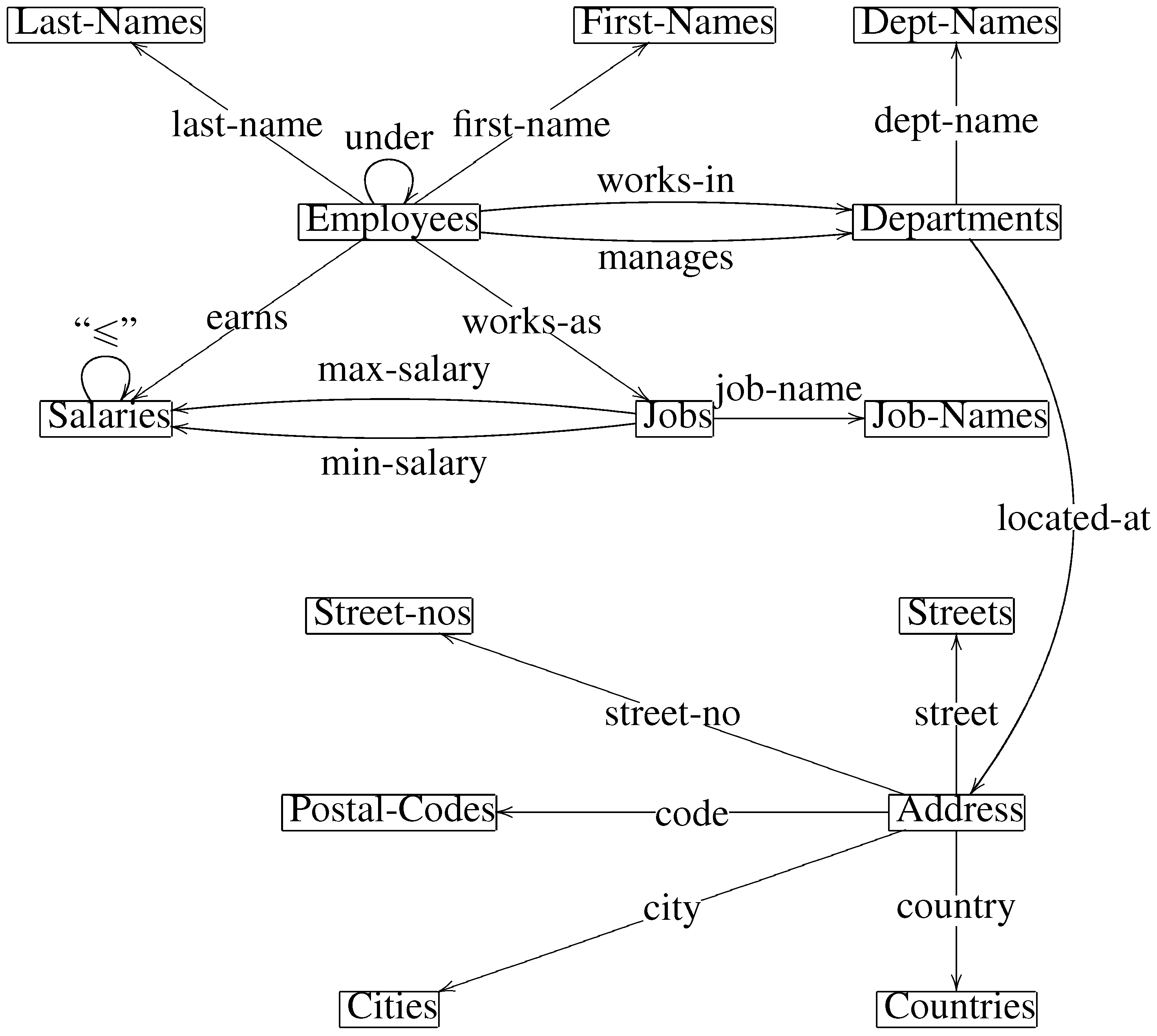
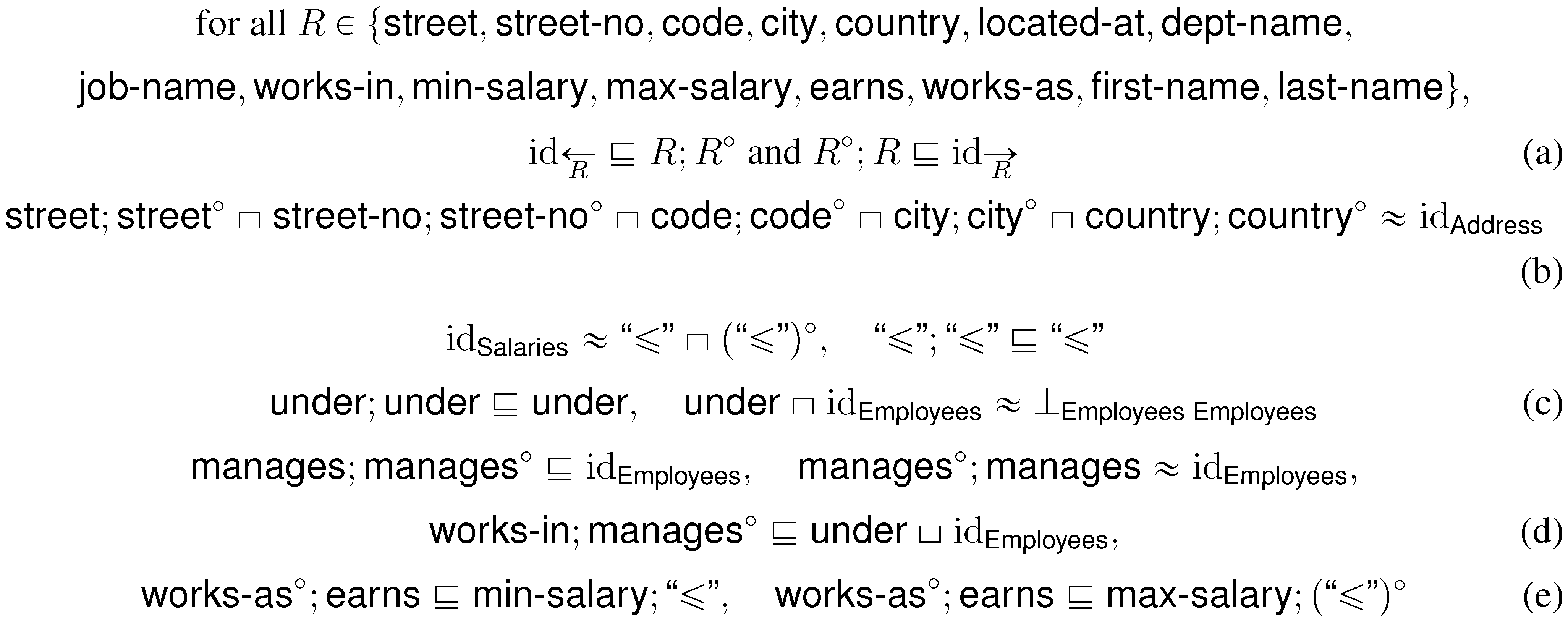
Example 1. 

A conceptual model $(\mathcal{G},\mathcal{E})$ loosely based on an example HR database of Oracle is depicted in Figure 1 (graph $\mathcal{G}$) and Figure 2 (equations $\mathcal{E}$). Equation (a) states that the arrows in the list are (total) maps; Equation (b) states that maps $\mathsf{\text{street}}$, $\mathsf{\text{street-no}}$, $\mathsf{\text{code}}$, $\mathsf{\text{city}}$ and $\mathsf{\text{country}}$ are jointly monic (that is an $\mathsf{\text{Address}}$ is uniquely determined by the values of these attributes). Equation (c) makes $‘‘\le ’’$ a linear order and $\mathsf{\text{under}}$ transitive (it is meant as a transitive closure of the chain of commands) and irreflexive relation. The first two equations in Equation (d) specify that ${\mathsf{\text{manages}}}^{\circ }$ is an injective map (i.e., each department has a manager, and no manager manages two different departments). Then, the last of equations in (d) link relations $\mathsf{\text{manages}}$ and $\mathsf{\text{under}}$ by specifying that either an employee is a manager of the department he/she works in or he/she is under the departmental manager. Finally, Equation (e) limits the wages by enforcing that an employee doing a certain job type may not earn less than the minimal wage nor more than the maximal wage associated with the given job type.

The model is intended to be interpreted in some PTBDI allegory. Each interpretation corresponds to some actual realization and state of the database. The choice of allegory determines the kind of database; different interpretations in the same allegory may be interpreted as different states of the same database. Interpretation of the allegorical conceptual model in $\mathcal{R}$ is the typical choice. In order to formulate the precise definition of interpretation, we first need the following simple observation:

Figure 1. An example of an allegorical conceptual model graph.

Figure 1. An example of an allegorical conceptual model graph.

Figure 2. Equations specifying the properties of relations from Figure 1.

Figure 2. Equations specifying the properties of relations from Figure 1.

Lemma 4. 

Let $\mathcal{G}$ be a graph, and let $\mathcal{A}$ be a PTBDI allegory. Let $F:\mathcal{G}\to \mathcal{A}$ be a graph morphism. Then, $F_o$ can be extended to a map ${\widehat{F}}_o:{\mathrm{Obj}}^E\left[\mathcal{G}\right]\to \mathrm{Obj}\left[\mathcal{A}\right]$ using induction on the ⊗-groupoid structure of ${\mathrm{Obj}}^E\left[\mathcal{G}\right]$; that is, by defining ${\widehat{F}}_o(A\otimes B)={\widehat{F}}_o(A)\otimes {\widehat{F}}_o(B)$ for all $A,B\in {\mathrm{Obj}}^E\left[\mathcal{G}\right]$. Similarly, $F_a$ can be extended to a map ${\widehat{F}}_a:{\mathcal{T}}_{\mathcal{G}}\to \mathrm{Arr}\left[\mathcal{A}\right]$ using induction on the structure of terms in ${\mathcal{T}}_{\mathcal{G}}$; that is, by defining ${\widehat{F}}_a({\mathrm{id}}_A)={\mathrm{id}}_{F_o(A)}$, ${\widehat{F}}_a(t_1;t_2)={\widehat{F}}_a(t_1);{\widehat{F}}_a(t_2)$, and so on.

The following remark clarifies the above lemma. Suppose that: is a subgraph contained in a graph $\mathcal{G}$, and that $F:\mathcal{G}\to \mathcal{A}$ is a graph morphism from $\mathcal{G}$ into a PTBDI allegory, $\mathcal{A}$, such that $F_a(T)\ne F_a(R);F_a(S)$. Consequently, by the above definition of the extension ${\widehat{F}}_a:{\mathcal{T}}_{\mathcal{G}}\to \mathrm{Arr}\left[\mathcal{A}\right]$ of $F_a$, we have ${\widehat{F}}_a(R;S):=F_a(R);F_a(S)\ne {\widehat{F}}_a(T)$, where ${\widehat{F}}_a(T):=F_a(T)$. Note that even if T is intended to be interpreted as a composition of R and S, this intention cannot be communicated through the structure of the graph, $\mathcal{G}$, and hence, it does not introduce any inconsistency in the extension of $F_a$. On the other hand, the intended identification of T with the composition of R and S can be declared through equations. In particular, if $(R;S\approx T)\in \mathcal{E}$, then F cannot be an interpretation of $(\mathcal{G},\mathcal{E})$, as defined below.

Definition 5. 

Let $(\mathcal{G},\mathcal{E})$ be an allegorical conceptual data model, and let $\mathcal{A}$ be a PTBDI allegory. A graph morphism $H:\mathcal{G}\to \mathcal{A}$ is called an interpretation of $(\mathcal{G},\mathcal{E})$ in $\mathcal{A}$ if ${\widehat{H}}_a(t_1)={\widehat{H}}_a(t_2)$ for all equations $(t_1\approx t_2)\in \mathcal{E}$. A set of all interpretations of $(\mathcal{G},\mathcal{E})$ is denoted by $\mathrm{Ipt}[\mathcal{G},\mathcal{E}]$, and the set of all interpretations in an allegory $\mathcal{A}$ is denoted by ${\mathrm{Ipt}}_{\mathcal{A}}[\mathcal{G},\mathcal{E}]$.

Reasoning about data is furnished by the following semantic definition of a derived equality:

Definition 6. 

Let $(\mathcal{G},\mathcal{E})$ be an allegorical conceptual model. We write $(\mathcal{G},\mathcal{E}){\vDash }_F{t}_1\approx t_2$, where F is an interpretation of $(\mathcal{G},\mathcal{E})$ if ${\widehat{F}}_a(t_1)={\widehat{F}}_a(t_2)$. We write $(\mathcal{G},\mathcal{E})\vDash t_1\approx t_2$ (the equality $t_1\approx t_2$ holds in $(\mathcal{G},\mathcal{E})$) if $(\mathcal{G},\mathcal{E}){\vDash }_F{t}_1\approx t_2$ for any interpretation F of $(\mathcal{G},\mathcal{E})$.

3. Modal Terms and Modal Interpretations

Recall that a modal similarity type $(\underline{\mathbb{S}},\rho )$ consists of a set, $\underline{\mathbb{S}}$, of symbols and a map $\rho :\underline{\mathbb{S}}\to \mathbb{N}$ called an arity. A frame $(\mathbb{M},\mathbb{R})$ with modal similarity type $(\underline{\mathbb{S}},\rho )$ is a set, $\mathbb{M}$, together with a family $\mathbb{R}:=\{{\mathbb{R}}_{\mathfrak{S}}\subseteq {\mathbb{M}}^{\rho (\mathfrak{S})+1}|\mathfrak{S}\in \underline{\mathbb{S}}\}$ of relations.

Let $\mathcal{G}$ be a graph, and let $(\underline{\mathbb{S}},\rho )$ be a modal similarity type. We extend the set, ${\mathcal{T}}_{\mathcal{G}}$, of allegorical terms associated with $\mathcal{G}$ to a set, ${\mathcal{T}}_{\mathcal{G}}^{\underline{\mathbb{S}},\rho }$, of modal allegorical terms of modal similarity type $(\underline{\mathbb{S}},\rho )$ by introducing new term constructors called modal operators: for each $\mathfrak{S}\in \underline{\mathbb{S}}$, such that $\rho (\mathfrak{S})\ge 1$, and each term $t_1,\dots ,t_{\rho (\mathfrak{S})}\in {\mathcal{T}}_{\mathcal{G}}^{\underline{\mathbb{S}},\rho }$ such that $\overleftarrow{t_1}=\overleftarrow{t_2}=\cdots =\overleftarrow{t_{\rho (\mathfrak{S})}}$ and $\overrightarrow{t_1}=\overrightarrow{t_2}=\cdots =\overrightarrow{t_{\rho (\mathfrak{S})}}$ also terms ${\Delta }_{\mathfrak{S}}(t_1,\dots ,t_{\rho (\mathfrak{S})}),{\nabla }_{\mathfrak{S}}(t_1,\dots ,t_{\rho (\mathfrak{S})})\in {\mathcal{T}}_{\mathcal{G}}^{\underline{\mathbb{S}},\rho }$. We also declare:

$$\begin{array}{c}\overleftarrow{{\Delta }_{\mathfrak{S}}(t_1,\dots ,t_{\rho (\mathfrak{S})})}=\overleftarrow{t_1}=\overleftarrow{{\nabla }_{\mathfrak{S}}(t_1,\dots ,t_{\rho (\mathfrak{S})})}\\ \overrightarrow{{\Delta }_{\mathfrak{S}}(t_1,\dots ,t_{\rho (\mathfrak{S})})}=\overrightarrow{t_1}=\overrightarrow{{\nabla }_{\mathfrak{S}}(t_1,\dots ,t_{\rho (\mathfrak{S})})}\end{array}$$

(i.e., modal operators associate arrows with arrows from the same hom-set) so that the terms with modal operators can be used as subterms. Arity zero modal operators (that is, modal constants) require special treatment. For all $\mathfrak{S}\in \underline{\mathbb{S}}$ such that $\rho (\mathfrak{S})=0$, and all pairs of objects $A,B\in \mathrm{Obj}\left[\mathcal{G}\right]$, we declare ${\Delta }_{\mathfrak{S}}^{AB}$ to be a term in ${\mathcal{T}}_{\mathcal{G}}^{\underline{\mathbb{S}},\rho }$ with $\overleftarrow{{\Delta }_{\mathfrak{S}}^{AB}}=A$ and $\overrightarrow{{\Delta }_{\mathfrak{S}}^{AB}}=B$.

Definition 7. 

Let $(\mathbb{M},\mathbb{R})$ be a frame of similarity type $(\underline{\mathbb{S}},\rho )$; let $\mathcal{A}$ be a locally complete PTBDI allegory, and let $(\mathcal{G},\mathcal{E})$ be an allegorical conceptual data model. A modal interpretation $(\Phi ,\mathsf{{\rm Y}},ı)$ of $(\mathcal{G},\mathcal{E})$ in $\mathcal{A}$ with frame $(\mathbb{M},\mathbb{R})$ consists of a family of interpretations ${\left\{{\Phi }^m\right\}}_{m\in \mathbb{M}}\subseteq {\mathrm{Ipt}}_{\mathcal{A}}[\mathcal{G},\mathcal{E}]$, a map $\mathsf{{\rm Y}}:{\mathrm{Obj}}^E\left[\mathcal{G}\right]\to \mathrm{Obj}\left[\mathcal{A}\right]$ and a map $ı:\mathbb{M}\times {\mathrm{Obj}}^E\left[\mathcal{G}\right]\to \mathrm{Arr}\left[\mathcal{A}\right]$, where we denote ${ı}_A^m:=ı(m,A)$, satisfying, for all $A,B\in {\mathrm{Obj}}^E\left[\mathcal{G}\right]$ and $m\in \mathbb{M}$:

$$\begin{array}{c}{ı}_A^m;{({ı}_A^m)}^{\circ }={\mathrm{id}}_{\overleftarrow{{ı}_A^m}},{({ı}_A^m)}^{\circ };{ı}_A^m⊑{\mathrm{id}}_{\overrightarrow{{ı}_A^m}},\overleftarrow{{ı}_A^m}={\widehat{\Phi }}_o^m(A),\overrightarrow{{ı}_A^m}=\mathsf{{\rm Y}}(A)\end{array}$$

(10a)

$$\begin{array}{c}\mathsf{{\rm Y}}(A\otimes B)=\mathsf{{\rm Y}}(A)\otimes \mathsf{{\rm Y}}(B)\end{array}$$

(10b)

$$\begin{array}{c}{ı}_{A\otimes B}^m=\left({\widehat{\Phi }}_a^m({\pi }_A^{AB});{ı}_A^m;{\left({\pi }_{\mathsf{{\rm Y}}(A)}^{\mathsf{{\rm Y}}(A)\mathsf{{\rm Y}}(B)}\right)}^{\circ }\right)\sqcap \left({\widehat{\Phi }}_a^m({\pi }_B^{AB});{ı}_B^m;{\left({\pi }_{\mathsf{{\rm Y}}(B)}^{\mathsf{{\rm Y}}(A)\mathsf{{\rm Y}}(B)}\right)}^{\circ }\right)\end{array}$$

(10c)

We denote by ${\mathfrak{ModInt}}_{\mathcal{A}}^{\mathbb{M},\mathbb{R}}[\mathcal{G},\mathcal{E}]$ the set of all modal interpretations of $(\mathcal{G},\mathcal{E})$ in $\mathcal{A}$ with frame $(\mathbb{M},\mathbb{R})$.

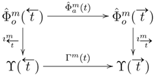
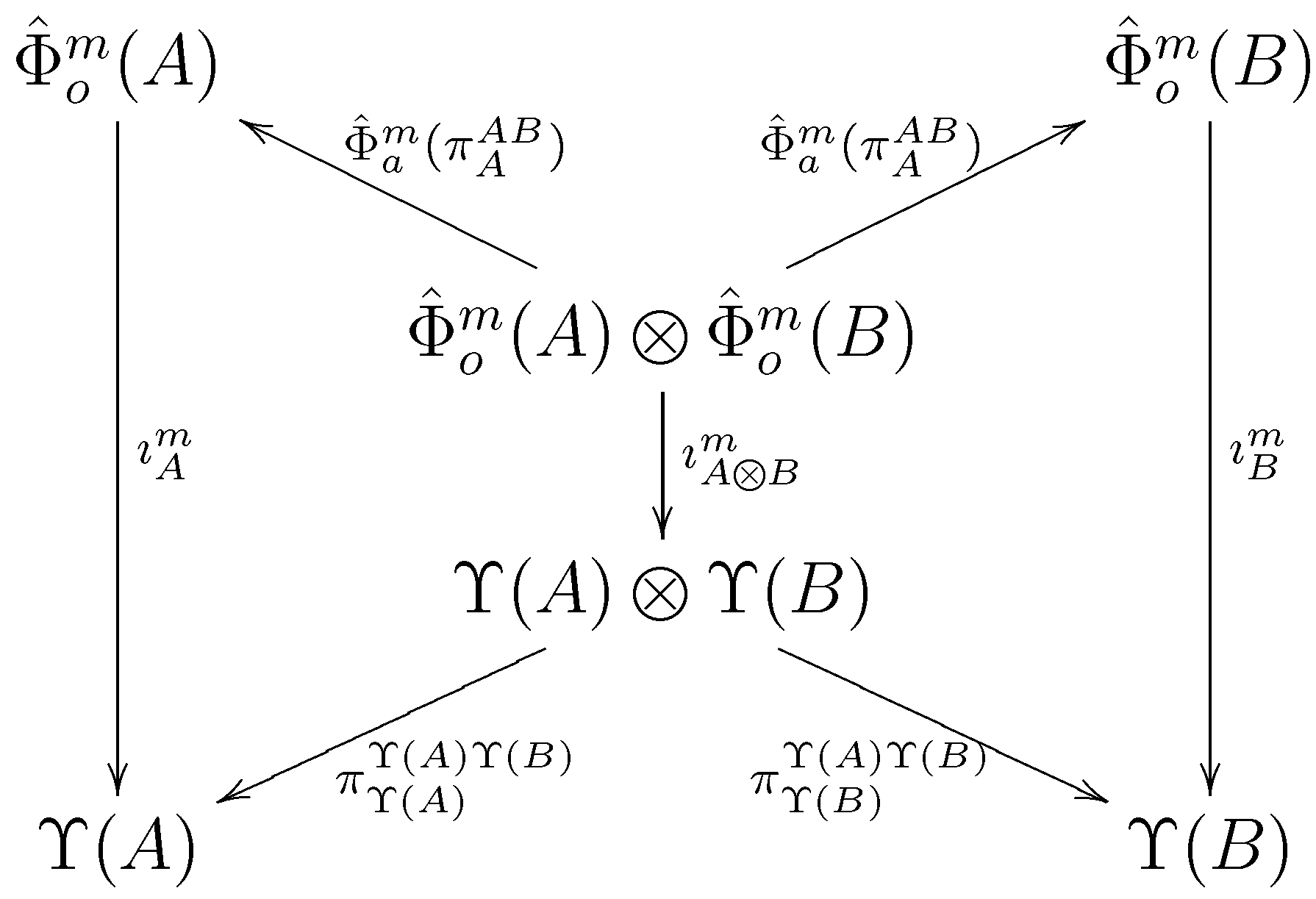
The last of the equalities (10) specifies ${ı}_{A\otimes B}^m$ to be a unique map which makes a diagram in Figure 3 commute (cf. Equation (4)). In fact, Formula (10c) could be taken as a definition of ${ı}_{A\otimes B}^m$, because it guarantees by itself that ${ı}_{A\otimes B}^m$ is an injective map. Indeed, ${ı}_{A\otimes B}^m$ as defined by Equation (10c) is a map because ${\widehat{\Phi }}_a^m({\pi }_A^{AB});{ı}_A^m$ and ${\widehat{\Phi }}_a^m({\pi }_B^{AB});{ı}_B^m$ are maps and ${\pi }_{\mathsf{{\rm Y}}(A)}^{\mathsf{{\rm Y}}(A)\mathsf{{\rm Y}}(B)}$, ${\pi }_{\mathsf{{\rm Y}}(B)}^{\mathsf{{\rm Y}}(A)\mathsf{{\rm Y}}(B)}$ are projections for a relational product. It remains to prove that ${ı}_{A\otimes B}^m;{({ı}_{A\otimes B}^m)}^{\circ }⊑{\mathrm{id}}_{{\widehat{\Phi }}_o^m(A)\otimes {\widehat{\Phi }}_o^m(B)}$:

$$\begin{array}{cc}& {ı}_{A\otimes B}^m;{({ı}_{A\otimes B}^m)}^{\circ }\hfill \\ \hfill ⊑& \left\{\text{Composition}\text{and}\text{reciprocation}\text{are}\text{monotonic}\right\}\hfill \\ & \left({\widehat{\Phi }}_a^m({\pi }_A^{AB});{ı}_A^m;{\left({\pi }_{\mathsf{{\rm Y}}(A)}^{\mathsf{{\rm Y}}(A)\mathsf{{\rm Y}}(B)}\right)}^{\circ }\right);{\left({\widehat{\Phi }}_a^m({\pi }_A^{AB});{ı}_A^m;{\left({\pi }_{\mathsf{{\rm Y}}(A)}^{\mathsf{{\rm Y}}(A)\mathsf{{\rm Y}}(B)}\right)}^{\circ }\right)}^{\circ }\hfill \\ \hfill =& \left\{\text{Properties}\text{of}{(·)}^{\circ }\right\}\hfill \\ & {\widehat{\Phi }}_a^m({\pi }_A^{AB});{ı}_A^m;{\left({\pi }_{\mathsf{{\rm Y}}(A)}^{\mathsf{{\rm Y}}(A)\mathsf{{\rm Y}}(B)}\right)}^{\circ };{\pi }_{\mathsf{{\rm Y}}(A)}^{\mathsf{{\rm Y}}(A)\mathsf{{\rm Y}}(B)};{ı}_A^{m\circ };{\widehat{\Phi }}_a^m{({\pi }_A^{AB})}^{\circ }\hfill \\ \hfill ⊑& \{{\pi }_{\mathsf{{\rm Y}}(A)}^{\mathsf{{\rm Y}}(A)\mathsf{{\rm Y}}(B)}\text{is}\text{functional}\text{and}‘‘;’’\text{is}\text{monotonic}\}\hfill \\ & {\widehat{\Phi }}_a^m({\pi }_A^{AB});{ı}_A^m;{ı}_A^{m\circ };{\widehat{\Phi }}_a^m{({\pi }_A^{AB})}^{\circ }\hfill \\ \hfill =& \left\{\text{Because}{ı}_A^m\text{is}\text{an}\text{injective}\text{map}\right\}\hfill \\ & {\widehat{\Phi }}_a^m({\pi }_A^{AB});{\widehat{\Phi }}_a^m{({\pi }_A^{AB})}^{\circ }\hfill \end{array}$$

Similarly, exchanging A and B, we prove the inequality

$${ı}_{A\otimes B}^m;{({ı}_{A\otimes B}^m)}^{\circ }⊑{\widehat{\Phi }}_a^m({\pi }_B^{AB});{\widehat{\Phi }}_a^m{({\pi }_B^{AB})}^{\circ }$$

Hence,

$$\begin{array}{cc}& {ı}_{A\otimes B}^m;{({ı}_{A\otimes B}^m)}^{\circ }\hfill \\ \hfill ⊑& \{\text{because}\sqcap \text{is}\text{infimum}\}\hfill \\ & \left({\widehat{\Phi }}_a^m({\pi }_A^{AB});{\widehat{\Phi }}_a^m{({\pi }_A^{AB})}^{\circ }\right)\sqcap \left({\widehat{\Phi }}_a^m({\pi }_B^{AB});{\widehat{\Phi }}_a^m{({\pi }_B^{AB})}^{\circ }\right)\hfill \\ \hfill =& \{{\widehat{\Phi }}_a^m({\pi }_A^{AB})\text{and}{\widehat{\Phi }}_a^m({\pi }_B^{AB})\text{are}\text{jointly}\text{monic}\}\hfill \\ & {\mathrm{id}}_{{\widehat{\Phi }}_o^m(A)\otimes {\widehat{\Phi }}_o^m(B)}\hfill \end{array}$$

as desired.

Observe that a modal interpretation $(\Phi ,\mathsf{{\rm Y}},ı)$ defines a family of maps ${\{{\Gamma }^m:{\mathcal{T}}_{\mathcal{G}}\to \mathcal{A}\}}_{m\in \mathbb{M}}$ given explicitly by:

$$\begin{array}{c}{\Gamma }_a^m(t)={{ı}_{\overleftarrow{t}}^m}^{\circ };{\widehat{\Phi }}_a^m(t);{ı}_{\overrightarrow{t}}^m,t\in {\mathcal{T}}_G\end{array}$$

(11)

Alternatively, ${\Gamma }^m$ is determined by the commutativity of the following family of diagrams (for all $t\in {\mathcal{T}}_{\mathcal{G}}$):

Figure 3. The construction of injection for a relational product (note that ${\widehat{\Phi }}_a^m({\pi }_A^{AB})={\pi }_{{\widehat{\Phi }}_o^m(A)}^{{\widehat{\Phi }}_o^m(A){\widehat{\Phi }}_o^m(B)}$ and ${\widehat{\Phi }}_a^m({\pi }_B^{AB})={\pi }_{{\widehat{\Phi }}_o^m(B)}^{{\widehat{\Phi }}_o^m(A){\widehat{\Phi }}_o^m(B)}$).

Figure 3. The construction of injection for a relational product (note that ${\widehat{\Phi }}_a^m({\pi }_A^{AB})={\pi }_{{\widehat{\Phi }}_o^m(A)}^{{\widehat{\Phi }}_o^m(A){\widehat{\Phi }}_o^m(B)}$ and ${\widehat{\Phi }}_a^m({\pi }_B^{AB})={\pi }_{{\widehat{\Phi }}_o^m(B)}^{{\widehat{\Phi }}_o^m(A){\widehat{\Phi }}_o^m(B)}$).

Lemma 8. 

${\Gamma }^m$ satisfies the following properties:

(1) 

For all $t_1,t_2\in {\mathcal{T}}_{\mathcal{G}}$, such that $\overleftarrow{t_1}=\overleftarrow{t_2}$ and $\overrightarrow{t_1}=\overrightarrow{t_2}$, if ${\Gamma }^m(t_1)={\Gamma }^m(t_2)$, then ${\widehat{\Phi }}_a^m(t_1)={\widehat{\Phi }}_a^m(t_2)$.

(2) 

For all $t_1,t_2\in {\mathcal{T}}_{\mathcal{G}}$, such that $\overleftarrow{t_1}=\overleftarrow{t_2}$ and $\overrightarrow{t_1}=\overrightarrow{t_2}$, we have ${\Gamma }^m(t_1\sqcap t_2)={\Gamma }^m(t_1)\sqcap {\Gamma }^m(t_2)$ and ${\Gamma }^m(t_1\bigsqcup t_2)={\Gamma }^m(t_1)\bigsqcup {\Gamma }^m(t_2)$.

(3) 

For all $t_1,t_2\in {\mathcal{T}}_{\mathcal{G}}$ such that $\overrightarrow{t_1}=\overleftarrow{t_2}$, we have ${\Gamma }^m(t_1;t_2)={\Gamma }^m(t_1);{\Gamma }^m(t_2)$.

(4) 

For all $A,B\in {\mathrm{Obj}}^E\left[\mathcal{G}\right]$, the following properties hold:

$$\begin{array}{c}{\Gamma }^m({\mathrm{id}}_A)⊑{\mathrm{id}}_{\mathsf{{\rm Y}}(A)},{\Gamma }^m({\perp }_{AB})={\perp }_{\mathsf{{\rm Y}}(A)\mathsf{{\rm Y}}(B)},{\Gamma }^m({\top }_{AB})⊑{\top }_{\mathsf{{\rm Y}}(A)\mathsf{{\rm Y}}(B)}\\ {\Gamma }^m({\pi }_A^{AB})⊑{\pi }_{\mathsf{{\rm Y}}(A)}^{\mathsf{{\rm Y}}(A)\mathsf{{\rm Y}}(B)},{\Gamma }^m({\pi }_B^{AB})⊑{\pi }_{\mathsf{{\rm Y}}(B)}^{\mathsf{{\rm Y}}(A)\mathsf{{\rm Y}}(B)}\end{array}$$

Proof. 

ad. 1: Suppose that ${\Gamma }^m(t_1)={\Gamma }^m(t_2)$. Then:

$$\begin{array}{cc}\hfill {\widehat{\Phi }}_a^m(t_1)& ={ı}_{\overleftarrow{t_1}}^m;{{ı}_{\overleftarrow{t_1}}^m}^{\circ };{\widehat{\Phi }}_a^m(t_1);{ı}_{\overrightarrow{t_1}}^m;{{ı}_{\overrightarrow{t_1}}^m}^{\circ }\hfill \\ & ={ı}_{\overleftarrow{t_1}}^m;{\Gamma }^m(t_1);{{ı}_{\overrightarrow{t_1}}^m}^{\circ }\hfill \\ & ={ı}_{\overleftarrow{t_2}}^m;{\Gamma }^m(t_2);{{ı}_{\overrightarrow{t_2}}^m}^{\circ }\hfill \\ & ={\widehat{\Phi }}_a^m(t_2)\hfill \end{array}$$

ad. 2: ${\Gamma }^m(t_1\bigsqcup t_2)={\Gamma }^m(t_1)\bigsqcup {\Gamma }^m(t_2)$ follows immediately from the distributivity of composition over union. The composition does not distribute over the intersection. However, it is well known (see, e.g., [1]) that in any allegory $R(S\sqcap T)=RS\sqcap RT$ and $(S\sqcap T)R^{\circ }=S{R}^{\circ }\sqcap T{R}^{\circ }$ if R is functional, that is, if $R^{\circ }R⊑{\mathrm{id}}_{\overrightarrow{R}}$. Hence, the result follows from the injectivity of ${ı}_{\overleftarrow{t_1}}^m$ and ${ı}_{\overrightarrow{t_1}}^m$, which implies the functionality of ${{ı}_{\overleftarrow{t_1}}^m}^{\circ }$ and ${{ı}_{\overrightarrow{t_1}}^m}^{\circ }$.

ad. 3:

$$\begin{array}{cc}\hfill {\Gamma }^m(t_1);{\Gamma }^m(t_2)& ={{ı}_{\overleftarrow{t_1}}^m}^{\circ };{\widehat{\Phi }}_a^m(t_1);{ı}_{\overrightarrow{t_1}}^m;{{ı}_{\overleftarrow{t_2}}^m}^{\circ };{\widehat{\Phi }}_a^m(t_2);{ı}_{\overrightarrow{t_2}}^m\hfill \\ & ={{ı}_{\overleftarrow{t_1}}^m}^{\circ };{\widehat{\Phi }}_a^m(t_1);{\widehat{\Phi }}_a^m(t_2);{ı}_{\overrightarrow{t_2}}^m\hfill \\ & ={{ı}_{\overleftarrow{t_1}}^m}^{\circ };{\widehat{\Phi }}_a^m(t_1;t_2);{ı}_{\overrightarrow{t_2}}^m\hfill \\ & ={\Gamma }^m(t_1;t_2)\hfill \end{array}$$

ad. 4: ${\Gamma }^m({\mathrm{id}}_A)={ı}_A^{m\circ };{\mathrm{id}}_{{\widehat{\Phi }}_o^m(A)};{ı}_A^m={ı}_A^{m\circ };{ı}_A^m⊑{\mathrm{id}}_{\mathsf{{\rm Y}}(A)}$, as ${ı}_A^m$ is functional. The first of Equations (5) implies that ${\Gamma }^m({\perp }_{AB})={\perp }_{\mathsf{{\rm Y}}(A)\mathsf{{\rm Y}}(B)}$. Inequality ${\Gamma }^m({\top }_{AB})⊑{\top }_{\mathsf{{\rm Y}}(A)\mathsf{{\rm Y}}(B)}$ holds trivially. Then, (cf. Figure 3):

$$\begin{array}{cc}& {\Gamma }^m({\pi }_A^{AB})\hfill \\ \hfill =& {\left({ı}_{A\otimes B}^m\right)}^{\circ };{\widehat{\Phi }}_a^m({\pi }_A^{AB});{ı}_A^m\hfill \\ \hfill =& \left(\left({\pi }_{\mathsf{{\rm Y}}(A)}^{\mathsf{{\rm Y}}(A)\mathsf{{\rm Y}}(B)};{ı}_A^{m\circ };{\widehat{\Phi }}_a^m{({\pi }_A^{AB})}^{\circ }\right)\sqcap \left({\pi }_{\mathsf{{\rm Y}}(B)}^{\mathsf{{\rm Y}}(A)\mathsf{{\rm Y}}(B)};{ı}_B^{m\circ };{\widehat{\Phi }}_a^m{({\pi }_B^{AB})}^{\circ }\right)\right);{\widehat{\Phi }}_a^m({\pi }_A^{AB});{ı}_A^m\hfill \\ \hfill ⊑& {\pi }_{\mathsf{{\rm Y}}(A)}^{\mathsf{{\rm Y}}(A)\mathsf{{\rm Y}}(B)};{ı}_A^{m\circ };{\widehat{\Phi }}_a^m{({\pi }_A^{AB})}^{\circ };{\widehat{\Phi }}_a^m({\pi }_A^{AB});{ı}_A^m\hfill \\ \hfill ⊑& {\pi }_{\mathsf{{\rm Y}}(A)}^{\mathsf{{\rm Y}}(A)\mathsf{{\rm Y}}(B)};{ı}_A^{m\circ };{ı}_A^m\hfill \\ \hfill ⊑& {\pi }_{\mathsf{{\rm Y}}(A)}^{\mathsf{{\rm Y}}(A)\mathsf{{\rm Y}}(B)}\hfill \end{array}$$

☐

Note that ${\Gamma }^m$ does not in general preserve identities, tops, bottoms and relational product projections, and thus, it is not an interpretation. The objects $\mathsf{{\rm Y}}(A)$, for $A\in {\mathrm{Obj}}^E\left[\mathcal{G}\right]$ should be considered a representation of “total domains”—the collections of all possible values (whatever that means in a general allegory). On the other hand, ${\Phi }^m$ is an interpretation of the conceptual model of the database in the concrete world (say a moment of time), and in particular objects ${\Phi }_o^m(A)$ represent actual values stored in the database in the world m.

Note also that ${\Gamma }^m$ does not preserve implications in general. This is obvious, as, in particular, in $\mathcal{R}$, the complement $\neg {\Gamma }^m(t):={\Gamma }^m(t)\to {\perp }_{\mathsf{{\rm Y}}(\overleftarrow{t})\mathsf{{\rm Y}}(\overrightarrow{t})}$ in the arrow-set ${\mathrm{Arr}}_{\mathcal{A}}(\mathsf{{\rm Y}}(\overleftarrow{t}),\mathsf{{\rm Y}}(\overrightarrow{t}))$ is much larger than the embedding ${\Gamma }^m(\neg t)$ in ${\mathrm{Arr}}_{\mathcal{A}}(\mathsf{{\rm Y}}(\overleftarrow{t}),\mathsf{{\rm Y}}(\overrightarrow{t}))$ of the complement of ${\widehat{\Phi }}_a^m(t)$ in ${\mathrm{Arr}}_{\mathcal{A}}({\widehat{\Phi }}_o^m(\overleftarrow{t}),{\widehat{\Phi }}_o^m(\overrightarrow{t}))$. However, Lemma 10 alleviates that a bit. First, we need the following general result, interesting on its own.

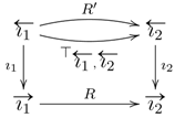
Lemma 9. 

Let ${ı}_1$ and ${ı}_2$ be injective maps in some allegory, $\mathcal{A}$, and suppose that the meet semilattice of arrows ${\mathrm{Arr}}_{\mathcal{A}}(\overleftarrow{{ı}_1},\overleftarrow{{ı}_2})$ contains the top element, ${\top }_{\overleftarrow{{ı}_1},\overleftarrow{{ı}_2}}$. Let $R\in {\mathrm{Arr}}_{\mathcal{A}}(\overrightarrow{{ı}_1},\overrightarrow{{ı}_2})$. Consider the following statements (see the diagram below for illustration):

(1) 

$R={ı}_1^{\circ };R^{\prime };{ı}_2$ for some $R^{\prime }\in {\mathrm{Arr}}_{\mathcal{A}}(\overleftarrow{{ı}_1},\overleftarrow{{ı}_2})$.

(2) 

$R={ı}_1^{\circ };{ı}_1;R$ and $R=R;{ı}_2^{\circ };{ı}_2$,

(3) 

$R⊑{ı}_1^{\circ };{\top }_{\overleftarrow{{ı}_1},\overleftarrow{{ı}_2}};{ı}_2$.

Statement (1) implies Statements (2) and (3), and Statement (3) implies Statements (1) and (2).

Proof. 

If $R={ı}_1^{\circ };R^{\prime };{ı}_2$, then, because $R^{\prime }⊑{\top }_{\overleftarrow{{ı}_1},\overleftarrow{{ı}_2}}$ and the composition is monotonic, we must also have $R={ı}_1^{\circ };R^{\prime };{ı}_2⊑{ı}_1^{\circ };{\top }_{\overleftarrow{{ı}_1},\overleftarrow{{ı}_2}};{ı}_2$. Furthermore, ${ı}_1^{\circ };{ı}_1;R={ı}_1^{\circ };{ı}_1;{ı}_1^{\circ };R^{\prime };{ı}_2={ı}_1^{\circ };R^{\prime };{ı}_2=R$ as ${ı}_1;{ı}_1^{\circ }={\mathrm{id}}_{\overleftarrow{{ı}_1}}$ and, similarly, $R=R;{ı}_2^{\circ };{ı}_2$. This finishes the proof of the first set of implications.

Assume now that $R⊑{ı}_1^{\circ };{\top }_{\overleftarrow{{ı}_1},\overleftarrow{{ı}_2}};{ı}_2$. We will prove first that ${ı}_1^{\circ };{ı}_1;R=R$. Because ${ı}_1$ is functional, i.e., ${ı}_1^{\circ };{ı}_1⊑{\mathrm{id}}_{\overrightarrow{{ı}_1}}$, and composition is monotonic, we have ${ı}_1^{\circ };{ı}_1;R⊑{\mathrm{id}}_{\overrightarrow{{ı}_1}};R=R$. Similarly, $R;{ı}_2^{\circ };{ı}_2⊑R$. In order to prove the other inequalities, we first define for any arrow, T, the domain of T:

$$\mathfrak{Dom}(T):={\mathrm{id}}_{\overleftarrow{T}}\sqcap T{T}^{\circ }$$

(12)

Recall ([1]) that $\mathfrak{Dom}$ has the following properties:

$$\begin{array}{c}\mathfrak{Dom}(TS)⊑\mathfrak{Dom}(T),\text{where}\overleftarrow{S}=\overrightarrow{T}\end{array}$$

(13a)

$$\begin{array}{c}T⊑S\Rightarrow \mathfrak{Dom}(T)⊑\mathfrak{Dom}(S)\end{array}$$

(13b)

$$\begin{array}{c}\forall H.H\subseteq {\mathrm{id}}_{\overleftarrow{T}}\Rightarrow \left((T⊑H;T)\equiv (\mathfrak{Dom}(T)⊑H)\right)\end{array}$$

(13c)

It follows from Formula (13c) that $R⊑{ı}_1^{\circ };{ı}_1;R$ if and only if $\mathfrak{Dom}(R)⊑{ı}_1^{\circ };{ı}_1$. By assumption, however, $R⊑{ı}_1^{\circ };{\top }_{\overleftarrow{{ı}_1},\overleftarrow{{ı}_2}};{ı}_2$, and so, by the transitivity of the order relation and the monotonicity of $\mathfrak{Dom}$ (Equation (13b)), it is enough to prove that $\mathfrak{Dom}({ı}_1^{\circ };{\top }_{\overleftarrow{{ı}_1},\overleftarrow{{ı}_2}};{ı}_2)⊑{ı}_1^{\circ };{ı}_1$. However, by Equation (13a), we have:

$$\mathfrak{Dom}({ı}_1^{\circ };{\top }_{\overleftarrow{{ı}_1},\overleftarrow{{ı}_2}};{ı}_2)⊑\mathfrak{Dom}({ı}_1^{\circ })={\mathrm{id}}_{\overleftarrow{{ı}_1^{\circ }}}\sqcap {ı}_1^{\circ };{({ı}_1^{\circ })}^{\circ }={\mathrm{id}}_{\overrightarrow{{ı}_1}}\sqcap {ı}_1^{\circ };{ı}_1={ı}_1^{\circ };{ı}_1$$

In order to prove that $R⊑R;{ı}_2^{\circ };{ı}_2$, first note that because reciprocation is monotonic and ${\top }_{\overleftarrow{{ı}_1},\overleftarrow{{ı}_2}}^{\circ }={\top }_{\overleftarrow{{ı}_2},\overleftarrow{{ı}_1}}$, if $R⊑{ı}_1^{\circ };{\top }_{\overleftarrow{{ı}_1},\overleftarrow{{ı}_2}};{ı}_2$, then $R^{\circ }⊑{ı}_2^{\circ };{\top }_{\overleftarrow{{ı}_2},\overleftarrow{{ı}_1}};{ı}_1$, and hence, by the just proven result, $R^{\circ }⊑{ı}_2^{\circ };{ı}_2;R^{\circ }$. Taking the reciprocation of both sides of this inequality yields $R⊑R;{ı}_2^{\circ };{ı}_2$ as desired.

Now, we are ready to prove the last implication. Assuming $R⊑{ı}_1^{\circ };{\top }_{\overleftarrow{{ı}_1},\overleftarrow{{ı}_2}};{ı}_2$, itfollows from the just proven result that ${ı}_1^{\circ };({ı}_1;R;{ı}_2^{\circ });{ı}_2=({ı}_1^{\circ };{ı}_1;R);{ı}_2^{\circ };{ı}_2=R;{ı}_2^{\circ };{ı}_2={ı}_2^{\circ };{ı}_2$. Hence, defining $R^{\prime }:={ı}_1;R;{ı}_2^{\circ }\in {\mathrm{Arr}}_{\mathcal{A}}(\overleftarrow{{ı}_1},\overleftarrow{{ı}_2})$ yields $R={ı}_1^{\circ };R^{\prime };{ı}_2$, as desired. ☐

Lemma 10. 

For all $t_1,t_2\in {\mathcal{T}}_{\mathcal{G}}$ such that $\overleftarrow{t_1}=\overleftarrow{t_2}$ and $\overrightarrow{t_1}=\overrightarrow{t_2}$, we have:

$${\Gamma }^m({\top }_{\overleftarrow{t_1}\overrightarrow{t_1}})\sqcap \left({\Gamma }^m(t_1)\to {\Gamma }^m(t_2)\right)={\Gamma }^m(t_1\to t_2)$$

Proof. 

Using explicit Formula (8) for an implication in a locally complete distributive allegory, and the distributivity law (6), we have:

$$\begin{array}{cc}& {\Gamma }^m({\top }_{\overleftarrow{t_1}\overrightarrow{t_1}})\sqcap \left({\Gamma }^m(t_1)\to {\Gamma }^m(t_2)\right)\hfill \\ \hfill =& {\Gamma }^m({\top }_{\overleftarrow{t_1}\overrightarrow{t_1}})\sqcap \underset{\genfrac{}{}{0pt}{}{R\in {\mathrm{Arr}}_{\mathcal{A}}(\mathsf{{\rm Y}}(\overleftarrow{t_1}),\mathsf{{\rm Y}}(\overrightarrow{t_1}))}{R\sqcap {\Gamma }^m(t_1)⊑{\Gamma }^m(t_2)}}{⨆}R\hfill \\ \hfill =& \underset{\genfrac{}{}{0pt}{}{R\in {\mathrm{Arr}}_{\mathcal{A}}(\mathsf{{\rm Y}}(\overleftarrow{t_1}),\mathsf{{\rm Y}}(\overrightarrow{t_1}))}{{\Gamma }^m({\top }_{\overleftarrow{t_1}\overrightarrow{t_1}})\sqcap R\sqcap {\Gamma }^m(t_1)⊑{\Gamma }^m(t_2)}}{⨆}\left({\Gamma }^m({\top }_{\overleftarrow{t_1}\overrightarrow{t_1}})\sqcap R\right)\hfill \end{array}$$

(*)

In the second equality, in order to change the ⨆ subscript, we made use of the fact that ${\Gamma }^m(t_1)⊑{\Gamma }^m({\top }_{\overleftarrow{t_1}\overrightarrow{t_1}})$. Note that by Lemma 9 ${\Gamma }^m({\top }_{\overleftarrow{t_1}\overrightarrow{t_1}})\sqcap R={{ı}_{\overleftarrow{t_1}}^m}^{\circ };R^{\prime };{ı}_{\overrightarrow{t_1}}^m$ for some $R^{\prime }\in {\mathrm{Arr}}_{\mathcal{A}}({\Phi }_o^m(\overleftarrow{t_1}),{\Phi }_o^m(\overrightarrow{t_1}))$. It follows immediately, because extending the set of which the supremum is taken increases the supremum value that:

$$(*)⊑\underset{\genfrac{}{}{0pt}{}{R^{\prime }\in {\mathrm{Arr}}_{\mathcal{A}}({\widehat{\Phi }}_o^m(\overleftarrow{t_1}),{\widehat{\Phi }}_o^m(\overrightarrow{t_1}))}{{{ı}_{\overleftarrow{t_1}}^m}^{\circ };R^{\prime };{ı}_{\overrightarrow{t_1}}^m\sqcap {\Gamma }^m(t_1)⊑{\Gamma }^m(t_2)}}{⨆}\left({{ı}_{\overleftarrow{t_1}}^m}^{\circ };R^{\prime };{ı}_{\overrightarrow{t_1}}^m\right)$$

(**)

Then, because the injectivity of ${ı}_{\overleftarrow{t_1}}^m$ and ${ı}_{\overrightarrow{t_1}}^m$ implies that ${{ı}_{\overleftarrow{t_1}}^m}^{\circ };R^{\prime };{ı}_{\overrightarrow{t_1}}^m\sqcap {\Gamma }^m(t_1)⊑{\Gamma }^m(t_2)$ if and only if $R^{\prime }\sqcap {\widehat{\Phi }}_a^m(t_1)⊑{\widehat{\Phi }}_a^m(t_2)$, we have that:

$$\begin{array}{cc}\hfill (**)& =\underset{\genfrac{}{}{0pt}{}{R^{\prime }\in {\mathrm{Arr}}_{\mathcal{A}}({\widehat{\Phi }}_o^m(\overleftarrow{t_1}),{\widehat{\Phi }}_o^m(\overrightarrow{t_1}))}{R^{\prime }\sqcap {\widehat{\Phi }}_a^m(t_1)⊑{\widehat{\Phi }}_a^m(t_2)}}{⨆}\left({{ı}_{\overleftarrow{t_1}}^m}^{\circ };R^{\prime };{ı}_{\overrightarrow{t_1}}^m\right)\hfill \\ & ={{ı}_{\overleftarrow{t_1}}^m}^{\circ };(\underset{\genfrac{}{}{0pt}{}{R^{\prime }\in {\mathrm{Arr}}_{\mathcal{A}}({\widehat{\Phi }}_o^m(\overleftarrow{t_1}),{\widehat{\Phi }}_o^m(\overrightarrow{t_1}))}{R^{\prime }\sqcap {\widehat{\Phi }}_a^m(t_1)⊑{\widehat{\Phi }}_a^m(t_2)}}{⨆}{R}^{\prime });{ı}_{\overrightarrow{t_1}}^m\hfill \\ & ={{ı}_{\overleftarrow{t_1}}^m}^{\circ };({\widehat{\Phi }}_a^m(t_1)\to {\widehat{\Phi }}_a^m(t_2));{ı}_{\overrightarrow{t_1}}^m\hfill \\ & ={{ı}_{\overleftarrow{t_1}}^m}^{\circ };{\widehat{\Phi }}_a^m(t_1\to t_2);{ı}_{\overrightarrow{t_1}}^m\hfill \\ & ={\Gamma }^m(t_1\to t_2)\hfill \end{array}$$

It remains to prove that:

$${\Gamma }^m({\top }_{\overleftarrow{t_1}\overrightarrow{t_1}})\sqcap \left({\Gamma }^m(t_1)\to {\Gamma }^m(t_2)\right)⊒{\Gamma }^m(t_1\to t_2)$$

The above inequality is equivalent to the conjunction of ${\Gamma }^m({\top }_{\overleftarrow{t_1}\overrightarrow{t_1}})⊒{\Gamma }^m(t_1\to t_2)$ (which holds by the monotonicity of ${\Gamma }^m$) and $\left({\Gamma }^m(t_1)\to {\Gamma }^m(t_2)\right)⊒{\Gamma }^m(t_1\to t_2)$. Using explicit Formula (8) for implication and the fact that decreasing the set for which the supremum is taken decreases the supremum value, we have:

$$\begin{array}{cc}\hfill {\Gamma }^m(t_1)\to {\Gamma }^m(t_2)=& \underset{\genfrac{}{}{0pt}{}{R\in {\mathrm{Arr}}_{\mathcal{A}}(\mathsf{{\rm Y}}(\overleftarrow{t_1}),\mathsf{{\rm Y}}(\overrightarrow{t_1}))}{R\sqcap {\Gamma }^m(t_1)⊑{\Gamma }^m(t_2)}}{⨆}R\hfill \\ \hfill ⊒& \underset{\genfrac{}{}{0pt}{}{R^{\prime }\in {\mathrm{Arr}}_{\mathcal{A}}({\widehat{\Phi }}_o^m(\overleftarrow{t_1}),{\widehat{\Phi }}_o^m(\overrightarrow{t_1}))}{{{ı}_{\overleftarrow{t_1}}^m}^{\circ };R^{\prime };{ı}_{\overrightarrow{t_1}}^m\sqcap {\Gamma }^m(t_1)⊑{\Gamma }^m(t_2)}}{⨆}\left({{ı}_{\overleftarrow{t_1}}^m}^{\circ };R^{\prime };{ı}_{\overrightarrow{t_1}}^m\right)\hfill \end{array}$$

The last expression is identical to (**), which is equal (as shown above) to ${\Gamma }^m(t_1\to t_2)$.  ☐

The following immediate corollary to Lemma 10 shows that for certain safe expressions, ${\Gamma }^m$ preserves implications:

Corollary 11. 

For all $t_1,t_2,t_3\in {\mathcal{T}}_{\mathcal{G}}$ with the same source and target and all $m\in \mathbb{M}$, we have:

$${\Gamma }^m(t_1)\sqcap {\Gamma }^m(t_2\to t_3)={\Gamma }^m(t_1)\sqcap \left({\Gamma }^m(t_2)\to {\Gamma }^m(t_3)\right)$$

We are now ready to define the interpretation of the modal formulas ${\mathcal{T}}_{\mathcal{G}}^{(\underline{\mathbb{S}},\rho )}$ in the allegory $\mathcal{A}$ using the interpretation $(\Phi ,\mathsf{{\rm Y}},ı)$.

Definition 12. 

Let $(\mathbb{M},\mathbb{R})$ be a frame of similarity type $(\underline{\mathbb{S}},\rho )$; let $\mathcal{A}$ be a locally complete PTBDI allegory, and let $(\mathcal{G},\mathcal{E})$ be an allegorical conceptual data model. A modal interpretation $(\Phi ,\mathsf{{\rm Y}},ı)$ of $(\mathcal{G},\mathcal{E})$ in $\mathcal{A}$ with frame $(\mathbb{M},\mathbb{R})$ defines for all $m\in \mathbb{M}$ a map ${\Xi }_{(\Phi ,\mathsf{{\rm Y}},ı)}^m:{\mathcal{T}}_{\mathcal{G}}^{(\underline{\mathbb{S}},\rho )}\to \mathrm{Arr}\left[\mathcal{A}\right]$ defined by induction on the structure of terms in ${\mathcal{T}}_{\mathcal{G}}^{\underline{\mathbb{S}},\rho }$ as follows (we omit the subscript whenever $(\Phi ,\mathsf{{\rm Y}},ı)$ is clear from the context):

• If $t\in \mathrm{Arr}\left[\mathcal{G}\right]$ or

  $$t\in \bigcup _{A,B\in {\mathrm{Obj}}^E\left[\mathcal{G}\right]}\{{\perp }_{AB},{\top }_{AB},{\pi }_A^{AB},{\pi }_B^{AB},{\mathrm{id}}_A\}$$

  then ${\Xi }^m(t):={\Gamma }^m(t)$.
• ${\Xi }^m(t_1;t_2)={\Xi }^m(t_1);{\Xi }^m(t_2)$, ${\Xi }^m(t_1\sqcap t_2)={\Xi }^m(t_1)\sqcap {\Xi }^m(t_2)$, ${\Xi }^m(t_1\bigsqcup t_2)={\Xi }^m(t_1)\bigsqcup {\Xi }^m(t_2)$, ${\Xi }^m(t_1\to t_2)={\Xi }^m(t_1)\to {\Xi }^m(t_2)$, ${\Xi }^m(t^{\circ })={\Xi }^m{(t)}^{\circ }$.
• If $\mathfrak{S}\in \underline{\mathbb{S}}$ is such that $\rho (\mathfrak{S})=0$ and $A,B\in {\mathrm{Obj}}^E\left[\mathcal{G}\right]$, then:

  $${\Xi }^m({\Delta }_{\mathfrak{S}}^{AB})=\left\{\begin{array}{cc}{\top }_{\mathsf{{\rm Y}}(A)\mathsf{{\rm Y}}(B)}\hfill & \text{if}m\in {\mathbb{R}}_{\mathfrak{S}}\hfill \\ {\perp }_{\mathsf{{\rm Y}}(A)\mathsf{{\rm Y}}(B)}\hfill & \text{if}m\notin {\mathbb{R}}_{\mathfrak{S}}\hfill \end{array}\right.$$
• If $\mathfrak{S}\in \underline{\mathbb{S}}$ is such that $\rho (\mathfrak{S})>0$ and $t_1,\dots ,t_{\rho (\mathfrak{S})}\in {\mathcal{T}}_{\mathcal{G}}^{\underline{\mathbb{S}},\rho }$ are such that $\overleftarrow{t_1}=\overleftarrow{t_2}=\cdots =\overleftarrow{t_{\rho (\mathfrak{S})}}$ and $\overrightarrow{t_1}=\overrightarrow{t_2}=\cdots =\overrightarrow{t_{\rho (\mathfrak{S})}}$, then:

  $$\begin{array}{cc}\hfill {\Xi }^m\left({\Delta }_{\mathfrak{S}}(t_1,\dots ,t_{\rho (\mathfrak{S})})\right)& =\underset{\genfrac{}{}{0pt}{}{m_1,\dots ,m_{\rho (\mathfrak{S})}\in \mathbb{M}}{\text{s.t.}{\mathbb{R}}_{\mathfrak{S}}(m,m_1,\dots ,m_{\rho (\mathfrak{S})})}}{⨆}\underset{1\le i\le \rho (\mathfrak{S})}{\sqcap }{\Xi }^{m_i}(t_i)\hfill \\ \hfill {\Xi }^m\left({\nabla }_{\mathfrak{S}}(t_1,\dots ,t_{\rho (\mathfrak{S})})\right)& =\underset{\genfrac{}{}{0pt}{}{m_1,\dots ,m_{\rho (\mathfrak{S})}\in \mathbb{M}}{\text{s.t.}{\mathbb{R}}_{\mathfrak{S}}(m,m_1,\dots ,m_{\rho (\mathfrak{S})})}}{\sqcap }\underset{1\le i\le \rho (\mathfrak{S})}{\sqcap }{\Xi }^{m_i}(t_i)\hfill \end{array}$$

Remark 1. 

Note that ${\Xi }^m$ preserves neither top elements, relational projections and identities nor implications (because ${\Gamma }^m$ does not preserve them either). Note, however, that by definition, $\overleftarrow{{\Xi }^m(t)}=\mathsf{{\rm Y}}(\overleftarrow{t})$ and $\overrightarrow{{\Xi }^m(t)}=\mathsf{{\rm Y}}(\overrightarrow{t})$ for all $t\in {\mathcal{T}}_{\mathcal{G}}^{(\underline{\mathbb{S}},\rho )}$.

Example 2. 

Here, we construct an allegorical counterpart of the basic modal logic. Let $(\mathbb{M},\mathbb{R})$ be a frame of similarity type $(\{\mathfrak{S}\},\mathfrak{S}\mapsto 1)$. Let $(\mathcal{G},\mathcal{E})$ be an allegorical conceptual data model and consider a modal interpretation $(\Phi ,\mathsf{{\rm Y}},ı)\in {\mathfrak{ModInt}}_{\mathcal{R}}^{\mathbb{M},\mathbb{R}}[\mathcal{G},\mathcal{E}]$. We denote customarily $\diamond R:={\Delta }_{\mathfrak{S}}(t)$ and $\square R:={\nabla }_{\mathfrak{S}}(t)$ for all $t\in {\mathcal{T}}_{\mathcal{G}}^{\mathfrak{S},\mathfrak{S}\mapsto 1}$. Let $a\in \mathsf{{\rm Y}}(\overleftarrow{t})$, $b\in \mathsf{{\rm Y}}(\overrightarrow{t})$. Then:

$$\begin{array}{c}a\left({\Xi }^m(\diamond t)\right)b\equiv \exists m^{\prime }\in \mathbb{M}.{\mathbb{R}}_{\mathfrak{S}}(m,m^{\prime })\wedge a\left({\Xi }^{m^{\prime }}(t)\right)b\\ a\left({\Xi }^m(\square t)\right)b\equiv \forall m^{\prime }\in \mathbb{M}.{\mathbb{R}}_{\mathfrak{S}}(m,m^{\prime })\Rightarrow a\left({\Xi }^{m^{\prime }}(t)\right)b\end{array}$$

Note that the above formulas are the same as in the definition of satisfaction of modal operators in the (first-order) basic modal logic (see, e.g., [19,20]).

Example 3. 

In this example, we will consider modal interpretations in the allegory $\mathcal{R}\left[L\right]$ where L is a locale, of locale-valued relations (see, e.g., [1]). In $\mathcal{R}\left[L\right]$, objects are sets, and for any $A,B\in \mathrm{Obj}\left[\mathcal{R}\right[L\left]\right]$, the hom-set ${\mathrm{Arr}}_{\mathcal{R}\left[L\right]}(A,B)$ consists of maps $R:A\times B\to L$. Locale-valued relations are usually interpreted as fuzzy relations, where the value, $R(a,b)$, gives the degree to which the relation, R, between a and b actually holds. Composition for $R,S\in \mathrm{Arr}\left[R\right[L\left]\right]$ such that $\overrightarrow{R}=\overleftarrow{S}$, is given by:

$$(RS)(a,c):=\underset{b\in \overrightarrow{R}}{\bigvee }\left(R(a,b)\wedge S(b,c)\right)$$

(14)

For all $A\in \mathrm{Obj}\left[\mathcal{R}\right[L\left]\right]$, the identity morphisms are given explicitly by ${\mathrm{id}}_A(a,b):=\top$ if $a=b$ and ${\mathrm{id}}_A(a,b):=\perp$ if $a\ne b$. The intersection, union and reciprocation operators are defined in $\mathcal{R}\left[L\right]$ by $(R\sqcap S)(a,b):=R(a,b)\wedge S(a,b)$, $(R\bigsqcup S)(a,b):=R(a,b)\vee S(a,b)$, $R^{\circ }(a,b):=R(b,a)$.

Let us now consider the formulas defining modal interpretation in the same setting as in Example 2, but with $\mathcal{R}\left[L\right]$ instead of $\mathcal{R}$. Then:

$$\begin{array}{c}\left({\Xi }^m(\diamond t)\right)(a,b)=\underset{\genfrac{}{}{0pt}{}{m^{\prime }\in \mathbb{M}}{\text{s.t.}{\mathbb{R}}_{\mathfrak{S}}(m,m^{\prime })}}{\bigvee }\left({\Xi }^{m^{\prime }}(t)\right)(a,b)\\ \left({\Xi }^m(\square t)\right)(a,b)=\underset{\genfrac{}{}{0pt}{}{m^{\prime }\in \mathbb{M}}{\text{s.t.}{\mathbb{R}}_{\mathfrak{S}}(m,m^{\prime })}}{\bigwedge }\left({\Xi }^{m^{\prime }}(t)\right)(a,b)\end{array}$$

Sometimes, the modal operators associated directly to the frame relations are not enough. For instance (see Example 4), the counterpart of until and since operators from temporal logic cannot be expressed using the formalism described so far. Therefore, we allow one to extend the set of terms, ${\mathcal{T}}_{\mathcal{G}}$, to the set, ${\mathcal{T}}_{\mathcal{G}}^{\Omega }$, using an arbitrary set of constructors corresponding to the set of operators, Ω, instead of using only the constructors tied in a canonical way to frame relations and attaching to those operators arbitrary (though defined using frame relations) semantics.

Example 4. 

Let $(\mathbb{M},\{\le \})$ be a frame of similarity type $(\{\mathfrak{S}\},\mathfrak{S}\mapsto 1)$, such that ≤ is a linear order. Let $(\mathcal{G},\mathcal{E})$ be an allegorical conceptual data model. We extend ${\mathcal{T}}_{\mathcal{G}}$ to ${\mathcal{T}}_{\mathcal{G}}^{\{\mathcal{S},\mathcal{U}\}}$ by adding two new term constructors: For all terms $t_1,t_2\in {\mathcal{T}}_{\mathcal{G}}^{\{\mathcal{S},\mathcal{U}\}}$ such that $\overleftarrow{t_1}=\overleftarrow{t_2}$ and $\overrightarrow{t_1}=\overrightarrow{t_2}$, also $\mathcal{U}(t_1,t_2)\in {\mathcal{T}}_{\mathcal{G}}^{\{\mathcal{S},\mathcal{U}\}}$ ($t1$ until $t_2$) and $\mathcal{S}(t_1,t_2)\in {\mathcal{T}}_{\mathcal{G}}^{\{\mathcal{S},\mathcal{U}\}}$ ($t1$ since $t_2$).

Let $(\Phi ,\mathsf{{\rm Y}},ı)\in {\mathfrak{ModInt}}_{\mathcal{A}}^{(\mathbb{M},\mathbb{R})}[\mathcal{G},\mathcal{E}]$, and let $m\in \mathbb{M}$. Then, the semantics of $\mathcal{S}$ and $\mathcal{U}$ is given by:

$$\begin{array}{c}{\Xi }^m(\mathcal{U}(t_1,t_2))=\underset{m^{\prime }|m\le m^{\prime }}{⨆}\left({\Xi }^{m^{\prime }}(t_2)\sqcap \underset{m^{\prime \prime }|m\le m^{\prime \prime }<m^{\prime }}{\sqcap }{\Xi }^{m^{″}}(t_1)\right)\\ {\Xi }^m(\mathcal{S}(t_1,t_2))=\underset{m^{\prime }|m^{\prime }\le m}{⨆}\left({\Xi }^{m^{\prime }}(t_2)\sqcap \underset{m^{\prime \prime }|m^{\prime }<m^{\prime \prime }\le m}{\sqcap }{\Xi }^{m^{″}}(t_1)\right)\end{array}$$

where we denote $m<m^{\prime }\equiv m\le m^{\prime }\wedge m\ne m^{\prime }$. In particular, if $\mathcal{A}=\mathcal{R}$, then for all $a\in \mathsf{{\rm Y}}(\overleftarrow{t_1})$ and $b\in \mathsf{{\rm Y}}(\overrightarrow{t_1})$, those definitions boil down to the classical definition of the since and until temporal modalities:

$$\begin{array}{cc}& a\left({\Xi }^m(\mathcal{U}(t_1,t_2))\right)b\hfill \\ \hfill =& \exists m^{\prime }|m\le m^{\prime }.\left(a\left({\Xi }^{m^{\prime }}(t_2)\right)b\wedge \forall m^{″}|m\le m^{″}<m^{\prime }.{\Xi }^{m^{″}}(t_1)\right)\hfill \\ & a\left({\Xi }^n(\mathcal{S}(t_1,t_2))\right)b\hfill \\ \hfill =& \exists m^{\prime }|m^{\prime }\le m.\left(a\left({\Xi }^{m^{\prime }}(t_2)\right)b\wedge \forall m^{″}|m^{\prime }<m^{″}\le m.{\Xi }^{m^{″}}(t_1)\right)\hfill \end{array}$$

Formal equalities between terms from ${\mathcal{T}}_{\mathcal{G}}^{\underline{\mathbb{S}},\rho }$ can be used to specify the dependencies between data from different “worlds”, where the “world” can mean, depending on the application, a time moment or perhaps a database server instance. Here is the precise definition.

Definition 13. 

Let $t_1,t_2\in {\mathcal{T}}_{\mathcal{G}}^{(\underline{\mathbb{S}},\rho )}$; let $(\mathbb{M},\mathbb{R})$ be a frame of similarity type $(\underline{\mathbb{S}},\rho )$, and let the modal interpretation $(\Phi ,\mathsf{{\rm Y}},ı)\in {\mathfrak{ModInt}}_{\mathcal{A}}^{(\mathbb{M},\mathbb{R})}[\mathcal{G},\mathcal{E})]$. We say that a formal equality $t_1\approx t_2$ is satisfied in modal interpretation $(\Phi ,\mathsf{{\rm Y}},ı)$ at $m\in \mathbb{M}$ if ${\Xi }_{(\Phi ,\mathsf{{\rm Y}},ı)}^m(t_1)={\Xi }_{(\Phi ,\mathsf{{\rm Y}},ı)}^m(t_2)$, which we denote by $(\Phi ,\mathsf{{\rm Y}},ı){⊩}_m{t}_1\approx t_2$. We say that a formal equality $t_1\approx t_2$ is satisfied in modal interpretation $(\Phi ,\mathsf{{\rm Y}},ı)$, which we denote by $(\Phi ,\mathsf{{\rm Y}},ı)⊩t_1\approx t_2$ if $(\Phi ,\mathsf{{\rm Y}},ı){⊩}_m{t}_1\approx t_2$ for all $m\in \mathbb{M}$.

4. Applications to Database Modeling

In this section, we consider how our formalism can be used to express business rules and queries in the context of temporal and distributed databases. In all the examples, we use the allegorical conceptual model depicted in Figure 1 and Figure 2.

4.1. Temporal Databases

Here, we work with frame $(\mathbb{T},\mathbb{R})$ of similarity type $\{\mathbb{O},\rho \}$, where we denote $\mathbb{O}:=\{‘‘\le ’’,‘‘\ge ’’,‘‘<’’,‘‘>’’\}$, $\rho (‘‘\le ’’)=\rho (‘‘\ge ’’)=\rho (‘‘<’’)=\rho (‘‘>’’)=1$. We abbreviate $\le :={\mathbb{R}}_{‘‘\le ’’}$ and similarly for the other symbols. We assume that ≤ is a linear order on $\mathbb{T}$ and that <, > and ≥ are dependent on ≤ in the usual way. We interpret the set of worlds, $\mathbb{T}$, as the time axis, with ≤ being the linear time ordering.

Example 5. 

Consider the following business rule concerning the allegorical conceptual model $(\mathcal{G},\mathcal{E})$ depicted in Figure 1 and Figure 2: “A manager of a department must have worked in the department in the past and not as its manager”. For simplicity let us ignore the fact that this rule is impossible to realize for the new departments. We claim that this rule can be expressed as the following formal equality between terms in ${\mathcal{T}}_{\mathcal{G}}^{(\mathbb{O},\rho )}$:

$$\mathsf{\text{manages}}⊑{\Delta }_{‘‘>’’}\left(\mathsf{\text{works-in}}\sqcap \neg \mathsf{\text{manages}}\right)$$

(15)

where we denoted for brevity $\neg \mathsf{\text{manages}}:=(\mathsf{\text{manages}}\to {\perp }_{\mathsf{Employees}\mathsf{\text{Departmets}}})$. Indeed, let the modal interpretation $(\Phi ,\mathsf{{\rm Y}},ı)\in {\mathfrak{ModInt}}_{\mathcal{R}}^{(\mathbb{T},\mathbb{R})}[\mathcal{G},\mathcal{E}]$, and let $m\in \mathbb{T}$. Then:

$$(\Phi ,\mathsf{{\rm Y}},ı){⊩}_m\mathsf{\text{manages}}⊑{\Delta }_{‘‘>’’}\left(\mathsf{\text{works-in}}\sqcap \neg \mathsf{\text{manages}}\right)$$

is equivalent to the statement, that for all elements $e\in \mathsf{{\rm Y}}(\mathsf{\text{Employees}})$ and $d\in \mathsf{{\rm Y}}(\mathsf{\text{Departments}})$:

$$\begin{array}{cc}\hfill e{\Xi }^m(\mathsf{\text{manages}})d\Rightarrow & \exists m^{\prime }<m.e{\Xi }^{m^{\prime }}(\mathsf{\text{works-in}})d\wedge \neg \left(e{\Xi }^{m^{\prime }}(\mathsf{\text{manages}})d\right)\hfill \end{array}$$

which is a direct first-order rendering of the desired business rule, where we read $a{\Xi }^m(R)b$, as a is in relation b at the time m.

Note that in Equation (15), the negation was used in a “safe” way in accordance with Corollary 11.

Example 6. 

Suppose that we want to create a temporal query (that is, a term in ${\mathcal{T}}_{\mathcal{G}}^{(\mathbb{O},\rho )}$), the evaluation of which at some moment $m\in \mathbb{T}$ will return those employees, whose pay will not decrease in the future. One may use such a term as a part of a formal equality stating some business rule or as a query in a temporal database. We claim that the query can be expressed as follows:

$$\left(\mathsf{\text{earns}};{\Delta }_{‘‘<’’}\left(‘‘\le ’’;{\mathsf{\text{earns}}}^{\circ }\right)\right)\sqcap {\mathrm{id}}_{\mathsf{\text{Employees}}}$$

(16)

Note the unfortunate clash of symbols here: in the above formula, we have the arrow $‘‘\le ’’$ from the graph, $\mathcal{G}$, and the relation symbol, $‘‘<’’\in \mathbb{O}$. Any modal interpretation is bound to represent Term (16) as a coreflexive (that is contained in the identity) arrow. Coreflexive arrows are natural allegorical representations of subobjects (subsets) (see, e.g., [1]). In $\mathcal{R}$, if R is coreflexive, then by definition $\overleftarrow{R}=\overrightarrow{R}$ and for all $e,e^{\prime }\in \overleftarrow{R}$, we have $eR{e}^{\prime }\Rightarrow e=e^{\prime }$. One can associate with R the subset $\{e\in \overleftarrow{R}|eRe\}\subseteq \overleftarrow{R}$. Conversely, with a subset $V\subseteq U$, one can associate a coreflexive relation $R_V\subseteq {\mathrm{id}}_U$ defined by $eR{e}^{\prime }\equiv e=e^{\prime }\wedge e\in V$.

The correctness of the solution (16) of our problem depends on the following reasonable assumption: the object $\mathsf{\text{Salaries}}$ should be understood not as a collection of salaries really earned by someone, but rather as a (generalized) numerical domain (e.g., NUMBER(6,2)). Accordingly, its interpretation (as well as the interpretation of the linear order, $‘‘\le ’’$) should be constant, that is, we consider only those modal interpretations $(\Phi ,\mathsf{{\rm Y}},ı)$ of $(\mathcal{G},\mathcal{E})$ in which for all $m\in \mathbb{T}$, we have:

$$\begin{array}{c}{\widehat{\Phi }}_o^m(\mathsf{\text{Salaries}})=\mathsf{{\rm Y}}(\mathsf{\text{Salaries}}),{ı}_{\mathsf{\text{Salaries}}}^m={\mathrm{id}}_{\mathsf{{\rm Y}}(\mathsf{\text{Salaries}})},{\widehat{\Phi }}_a^m(‘‘\le ’’)=\le \end{array}$$

(17)

As in the previous example, we consider the query to satisfy the desired semantics if the modal interpretation in $\mathcal{R}$ turns out to be the translation into the first-order logic of the problem statement. Therefore, let us consider any $(\Phi ,\mathsf{{\rm Y}},ı)\in {\mathfrak{ModInt}}_{\mathcal{R}}^{(\mathbb{T},\mathbb{R})}[\mathcal{G},\mathcal{E}]$ satisfying Conditions (17). Let T denote Term (16). In this setting, $e\left({\Xi }^m(T)\right)e^{\prime }$ can be equivalently written using Definition 12 as:

$$\exists m^{\prime }>m.\exists s,s^{\prime }\in \mathsf{{\rm Y}}(\mathsf{\text{Salaries}}).e\left({\Xi }^m(\mathsf{\text{earns}})\right)s\wedge s\le s^{\prime }\wedge e^{\prime }\left({\Xi }^m(\mathsf{\text{earns}})\right)s^{\prime }\wedge e=e^{\prime }$$

4.2. Replicated Databases

Here, we consider applications of modal interpretations of allegorical conceptual data models to specifying properties of replicated databases. One of the frames a replicated database can be associated with is the frame $(\mathbb{DB},\{⇝\})$ of similarity type $\mathcal{D}:=(\{‘‘⇝’’\},\{‘‘⇝’’\mapsto 1\})$. Here, $\mathbb{DB}$ is the set of database servers, and $d⇝d^{\prime }$ means that d pushes data into $d^{\prime }$. To avoid problems with circular pushes and consistency, we assume that the graph of ⇝ is acyclic and that that there exists a unique master, that is a database, $d\in \mathbb{DB}$, such that there exists no $d^{\prime }\in \mathbb{DB}$, such that $d^{\prime }⇝d$. Applications can read any database, but only the master is directly modified. What remains is the specification of details of change propagation.

Example 7. 

We want to specify the following rule: deletions from the relation $\mathsf{\text{works-in}}$ are propagated within the updating transaction. However insertions are propagated after the end of the transaction. The solution can be easily seen to be as follows:

$$\mathsf{\text{works-in}}⊒{\nabla }_{‘‘⇝’’}(\mathsf{\text{works-in}})$$

Consider now the frame $(\mathbb{T}\times \mathbb{DB},\mathbb{R}\cup \{⇝\})$ of similarity type $\{\mathbb{O}\cup \{‘‘⇝’’\},{\rho }^{\prime }\}$, where ${\rho }^{\prime }{|}_{\mathbb{O}}=\rho$ and ${\rho }^{\prime }(‘‘⇝’’)=1$. Here, $\mathbb{T}$, $\mathbb{R}$$\mathbb{O}$ and ρ are like in SubSection 4.1, and ⇝ and $\mathbb{DB}$ are like above, except that both $\mathbb{R}$ and ⇝ are extended in a natural way as relations on Cartesian product $\mathbb{T}\times \mathbb{DB}$, e.g., $((m,d)<(m^{\prime },d^{\prime })):\equiv (m<m^{\prime })$ and $((m,d)⇝(m^{\prime },d^{\prime })):\equiv (d⇝d^{\prime })$.

Example 8. 

Here, we continue Example 7. Note that one cannot express the requirement that the inserts will be eventually propagated without temporal modalities, that is using the frame that was used in the previous example. One can do it, however, using the frame described above, combining the replicated database frame with the temporal frame from the previous subsection. The reader will easily verify that the appropriate equation is as follows:

$$\mathsf{\text{works-in}}⊑{\nabla }_{‘‘<’’}({\Delta }_{‘‘⇝’’}(\mathsf{\text{works-in}}))$$

5. Conclusions

We have presented a modal extension of a new allegorical conceptual data model, which interprets modal operators within an appropriate allegory. Our formalism can be seen as a generalization via the relational algebra of a limited form of a first-order modal logic with variable domains (see, e.g., [19]). We have given a few examples of applications of the modal extensions of our allegorical conceptual data model to specifying properties of temporal or distributed databases. We hope that those examples justify our conviction about the usefulness and expressiveness of our approach. More examples are needed, however, where the data should be naturally interpreted in allegories other than $\mathcal{R}$ or $\mathcal{R}\left[L\right]$ for some locale, L.

It will be also interesting to compare our approach with that of [21], where it is shown how to enrich an arbitrary institution [22] with modalities and many worlds semantics. To make this comparison possible, we are currently working on the institutional formulation of our allegorical data model.