Article

Change Detection Using Wavelets in Solution Monitoring Data for Nuclear Safeguards

Los Alamos National Laboratory, Los Alamos, NM 87545, USA
*
Author to whom correspondence should be addressed.
Axioms 2013, 2(2), 271-285; https://doi.org/10.3390/axioms2020271
Submission received: 24 April 2013 / Revised: 17 May 2013 / Accepted: 22 May 2013 / Published: 18 June 2013
(This article belongs to the Special Issue Wavelets and Applications)

Abstract

:
Wavelet analysis is known to be a good option for change detection in many contexts. Detecting changes in solution volumes that are measured with both additive and relative error is an important aspect of safeguards for facilities that process special nuclear material. This paper qualitatively compares wavelet-based change detection to a lag-one differencing option using realistic simulated solution volume data for which the true change points are known. We then show quantitatively that Haar wavelet-based change detection is effective for finding the approximate location of each change point, and that a simple piecewise linear optimization step is effective to refine the initial wavelet-based change point estimate.

1. Introduction

As a component of a safeguards system for nuclear material, solutions in a nuclear facility such as an aqueous reprocessing plant are monitored for change. A change in the measured tank volume over time indicates loss or gain of nuclear material. Such changes could be part of legal plant operation, or could indicate a diversion of nuclear material by an adversary. In addition, change points can be used to implement piecewise linear regression for effective data smoothing [1]. Therefore, it is important to identify the times that these changes occur.
In applications of wavelets for change detection, wavelet decomposition coefficients have been used to identify edges in images and change points in time series data [2,3]. In the context of solution monitoring (SM) for nuclear safeguards, wavelet analysis is an appealing option for change detection because wavelets are localized in time and frequency and can detect both abrupt and gradual changes.
Other statistical methods are available for change point detection in the SM application, such as monitoring successive differences of the time series. Section 2 gives additional background for the SM application. Section 3 describes our method. Section 4 qualitatively compares wavelet-based change detection to a lag-one differencing option using realistic simulated data for which the true change points are known. We then show quantitatively that Haar wavelet-based change detection is effective for finding the approximate location of each change point, and that a simple piecewise linear optimization step is effective to refine the initial wavelet-based change point estimate.

2. Background

This paper’s wavelet application is SM at large commercial aqueous reprocessing plants. It is understood that because nuclear material accountancy (NMA) measurement uncertainty increases as facility throughput increases, in spite of sustained efforts to reduce measurement uncertainty, it remains difficult to satisfy the International Atomic Energy Agency diversion detection goal for large throughput facilities [4].
NMA at a declared and safeguarded facility involves measuring facility inputs, outputs, and inventory to compute a material balance (MB) defined as MB = Tin + IbeginToutIend, where T is a transfer and I is an inventory. The main quantitative assessment of safeguards effectiveness is the measurement error standard deviation of the material balance, which can be related to the probability of detecting a specified loss of NM for specified false alarm probability [4].
Partly in response to shortcomings of NMA alone, process monitoring (PM) is used as an additional measure to bolster NMA [4]. While it is generally agreed that PM adds value to safeguards, its possible roles and benefits are not fully understood. The main goal for using PM in addition to NMA is to improve the ability to detect off-normal plant operation.
As an example of PM, SM is a type of PM in which masses and volumes are estimated from frequent in-process measurements. If each tank is regarded as a sub-MBA (material balance area), then transfers between tanks can be identified, segments of which can then be compared to compute transfer differences (TDs). A safeguards concern might then be raised if either these TDs or deviations in mass or volume data during “wait” modes become significant [5,6,7,8]. Average mass and volume TDs should be zero (perhaps following a bias adjustment) to within a historical limit that is a multiple of the standard deviation of the mass or volume TD, as should deviations during “wait” modes. A residual (residual = measured − predicted) is generated each time a mode (transfer or wait) is completed by any tank. Such residuals can be analyzed over time and over tanks.
Measurement error effects in real SM data suggest that the standard deviation of the mass and volume TD in tank-to-tank transfers is approximately 5 to 10 times larger than international target values [9] and tank calibration studies suggest [5,10,11]. Reasons for the larger-than-anticipated standard deviation in the mass and volume TDs include failure to adequately smooth the mass and volume data, imperfect event marking (this paper’s focus), and process variation effects such as varying evaporation rates, varying amounts of solution carryover due to pipes and pump behavior, and temperature changes that impact volume measurements [8]. One data smoothing option is to estimate each change point location and apply piecewise linear regression [1]. Therefore, this paper’s focus is on options to estimate change point locations, both for improved piecewise linear regression performance, and because the times of each transfer are of interest.
It is not anticipated that safeguards personnel will routinely evaluate the large amounts of data generated from monitoring all transfers and wait modes for all tanks. Instead, some type of monitoring system will flag only anomalous transfers and wait modes. In-tank dip tubes located at various tank heights measure pressures that can be converted to density and to volume via a level-to-volume calibration. Solution mass in the tank is then calculated as volume times density. For our purposes here, it is sufficient to consider only discrete time series of tank volume. Analysis of tank mass, for example, is similar.

3. Method

3.1. Data Description

In this paper, tank volumes used in SM are assumed to be well represented by a function of time, M(t), with additive and relative noise [5,10], as
M ( t ) = T ( t ) + T ( t ) e R + e A
e R N ( 0 , σ R )
e A N ( 0 , σ A )
That is, relative and additive random noises are generated from normal distributions with mean 0 and standard deviations σR and σA, respectively. Such simulated data represents a discrete time series of measurements (volume or mass) of aqueous solutions at a reprocessing facility [4,5,6,7,8].
The purpose of this analysis is to detect change points in the measurement data, M(t), without misdiagnosing noise as change points. Figure 1 is an example simulated dataset. Typical values for σR range from approximately 0.001 (0.1%) to 0.03. Typical values for σA depend on the measurement units and for the range of T values we consider, σA ranges from approximately 0.1 to 2 [5,10]. This paper uses nominal values of σA = 1 and σR = 0.015 for additive and relative errors, respectively; other values for σR and σA are also used when indicated in Section 4. Notice that there is no transform of Equation (1) that converts the measurement error model to purely additive error.
The simulated data in Figure 1 uses σA = 1 and σR = 0.015 and clearly includes four abrupt events over two tank cycles; each cycle has a receipt and a shipment. Because this data is simulated, the exact start and stop time indices of the events are known, which is useful because the change point estimates of event detection algorithms can then be compared to the known true values. Therefore, this data set and variations of it are used throughout this paper. For Figure 1, the data is generated at constant intervals. The first rise spans 10 data points (somewhat abrupt), while the second rise spans only 1 data point (very abrupt); the first drop spans 10 data points and the second drop spans 20 data points (more gradual).
Figure 1. Simulated data M(t) from Equation (1).
Axioms 02 00271 g001
Change detection algorithms can be applied to raw or smoothed data. However, because piecewise linear regression is among the best smoothing options [1], and applying piecewise linear regression requires estimation of change points, all results given here are obtained from raw (unsmoothed) data, to avoid the challenge of determining the smoother [12] that provides the best event detection ability.

3.2. Wavelets

Wavelet transformations are similar to Fourier transformations, but wavelets are localized in frequency and time. A wavelet family is an orthonormal basis created by varying parameters j and k of the basis { ψ j k ( t ) = 2 j / 2 ψ ( 2 j t - k )   with   j , k } . The mother wavelet 𝜓 can be any zero-mean oscillating function. One simple example of a family of wavelets is the Haar wavelet basis [13,14] shown in Figure 2. The discrete wavelet transform of the data M(t) is j Z k Z w j k ψ j k ( t ) , where w j k = R M ( t ) ψ j k ( t ) d t .
Figure 2. Wavelet function example. The Haar mother wavelet.
Axioms 02 00271 g002

3.3. Lag-One Differencing Change Detection

Our change detection goal is to recognize the start and stop times of shipments or receipts of nuclear material, and to identify whether there has been deliberate diversion or innocent loss of nuclear material using the associated estimated change in measurements. These shipments and receipts are called “events”.
A simple event-detection option is to declare that a sub-event occurs in M(t) over time steps t1 and t2 if Δ = | M ( t 2 ) - M ( t 1 ) | c > h , where c is a scale factor and h is a statistically determined threshold value used to differentiate events from noise [7]. The scale factor c can be defined as the empirical standard deviation of the ∆ values. Alternatively, if multiple events are present and c is intended to characterize the typical change rate during non-events, then c can be defined as a robust estimate of the standard deviation (see Section 3.4) of the ∆ values during non-events. If multiple sub-events occur over a contiguous set of time points, the sub-events are concatenated together to form a single event, such as a shipment that occurs over multiple time steps. This “lag-one differencing” option is simple and it is adequate for detecting abrupt events; however, it can fail to detect gradual events [7] as we will show.

3.4. Wavelet Change Detection

Wavelet change detection uses the wavelet coefficients wjk to locate change points. If a wavelet decomposition coefficient │wjk│ is above a predetermined “critical value”, it is assumed that the coefficient corresponds to a change point in the data. The optimal critical value depends on characteristics of the original data. As an example, Figure 3 shows example simulated data with a gradual receipt and shipment, and the corresponding wavelet coefficients at various resolution levels. Resolution level 1 is the finest resolution, corresponding to lag-one differencing. Resolution level 2 is the next finest resolution, and so on.
Figure 3. Simulated scaled volumes for one tank cycle and the wavelet coefficients at each of five resolutions. Horizontal threshold lines at ±5 are included. Resolution 4 or 5 work well for this example and for similar examples because the threshold can be selected to find only one outlier in the receipt change region and one outlier in the shipment change region. Plot (a) is the scaled volume versus the time index. Plots (b)–(f) are the corresponding wavelet coefficients at 5 different resolutions.
Axioms 02 00271 g003aAxioms 02 00271 g003b
One requirement when using wavelets is that the data must be of a dyadic length (2j for j ∈ ℤ). SM data is plentiful so it is easy to break the data into dyadic sections. All simulated datasets have dyadic length (usually 256, 512, or 1024) to keep the analysis simple. Wavelet change detection can be done at varying resolution levels. For our SM data, using the Haar-based wavelet, we find it is easiest to detect abrupt events at low resolution numbers (which correspond to high resolution), and to detect gradual events at higher resolution numbers, as illustrated in Figure 4. In Figure 4, the first tank cycle has an abrupt receipt that is most easily detected at low resolution number and the second tank cycle has a gradual receipt that is most easily detected at high resolution number. The coefficients w1–w4 are wavelet coefficients at resolutions 1 to 4. Figure 4 is similar to Figure 8 in [15].
Figure 4. Haar-wavelet based change detection for two tank cycles. In the first cycle, there is an abrupt receipt and gradual shipment. In the second cycle, there is a gradual receipt and gradual shipment. Wavelet coefficients w1–w4 can be used alone or together for change detection.
Axioms 02 00271 g004
Because of the need to detect both abrupt and gradual changes, one often decomposes the signal at many resolution levels and extracts information about the signal/data using any relevant resolution level. All resolution levels can be evaluated simultaneously to monitor wavelet coefficients at many resolution levels [13,14,15,16,17,18,19,20,21,22,23,24,25]. In Section 4 we show that because our receipt and ship events all have a start and stop index, performance is best if we first locate a change region within which a change point occurs, and then refine the initial estimate of each change point using data only from the change region. We find that using moderately high resolution is best in our SM application for locating change regions. For example, Figure 3 suggests that moderate resolutions of 4 or 5 are effective for finding change regions, which is what we use in our numerical examples.
Wavelet coefficients follow a probability distribution with parameters that depend on the data or signal to be decomposed [25]. As the resolution increases, the distribution of the wavelet coefficients becomes better approximated by a normal distribution [18,19], which we confirmed using frequency histograms for simulated data such as in Figure 3. To identify the wavelet coefficients wjk that correspond to change regions, we use a simulation-based approach to estimate the distribution of wavelet coefficients and to find an effective resolution j for change-region identification. We standardize wjk to approximately unit standard deviation by dividing by a robust estimate (that down weights outliers) of the standard deviation σ ^ w j (we used the function cov.mve in R [26] to calculate a robust estimate σ ^ w j ). The time index k is inferred to be an outlier at resolution j, if w j k σ ^ w j k a for threshold a that is also chosen by simulation. The appropriate a value varies, depending on the resolution level. We found by extensive simulation using variations of SM data such as in Figure 1 and Figure 4 that a moderate resolution of 4 is adequate for both abrupt and gradual SM events.

4. Comparison of Change-Point Detection Methods in Simulated SM Data

The first step in our change point detection approach is to infer the number of change points in a region of data and the approximate time of each change point. The second step is to refine the initial estimates of the time of each change point.
Functions such as the breakpoint function in R [26] attempt to both infer the number of change points and their approximate times using a piecewise linear change detection technique described in [21]. Alternatively, wavelet-based change detection and the lag-one differencing option can infer the number of change points and their approximate times.

4.1. Finding the Correct Number of Change Points and the Approximate Times of Each Change Point

Wavelet change detection performance [23] can be measured on the basis of three criteria: (1) Good detection (low rate of false positives and false negatives in locating change points); (2) Good localization (accurate estimate of the exact change point location); and (3) Low response per change point, which expands on (1) by considering the number of change points inferred to be associated with a single true change point. References [13,14,15,16,17,18,19,20,21,22,23,24,25] are among the many references that describe wavelet change point detection using some type of synthesis of wavelet coefficients at each of multiple scales. For example, [23] presented a computational approach to synthesize wavelet coefficients over multiple scales. Reference [15] presented a different computational approach for signals that are piecewise polynomial (such as our SM signals that are piecewise linear). Because piecewise polynomial signals impact wavelet coefficients at multiple scales (see Figure 3 and Figure 4), [15] relied on a piecewise polynomial approximation that departed from conventional orthogonal wavelet bases.
In our SM signals, we know there is a distinct start and stop time index during which a receipt or shipment occurs. Therefore, our approach is to find the change region associated with each event (receipt or shipment) and then find the start and stop indices of that event. Candidate methods are then compared based on their ability to locate each approximate change “region”, without any “breakdown”, which is our informal term for failure to infer the correct number of change regions [7].
However, in multiple simulations of SM data, we found that no method, not the breakpoints method, not the simple lag-one differencing, and no multi-resolution wavelet-based method, gives adequately reliable change detection for the desired range of σR and σA values unless the correct number of change points is known. For example, 
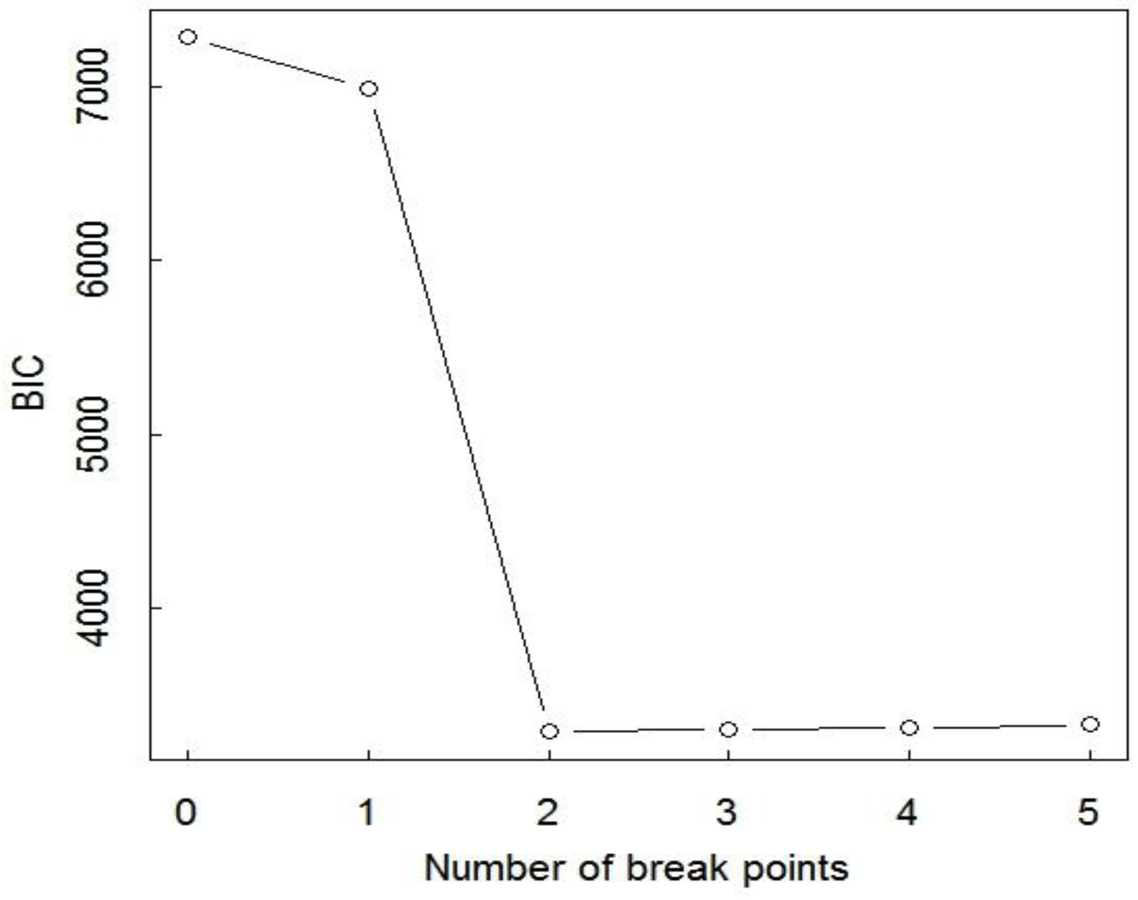
Figure 5 illustrates that breakpoints finds only two of the four change points in the first tank cycle data such as in Figure 1. The Bayesian information criterion (BIC) is used in breakpoints to infer the number of change points. The BIC is defined as BIC = −2log(maxlikelihood) + plog(n), where maxlikelihood is the maximum likelihood (corresponds to the usual least squares regression estimate in the case of Gaussian data) and p is the number of model parameters to penalize for the number of breakpoints. The model having the smallest BIC is preferred, and changes in BIC of less than approximately 10 are commonly assumed to be noise. Therefore, Figure 5 shows that breakpoints selected only two of four change points, failing to detect a slope change within each transfer. In addition, breakpoints is slow to run on 1024 data points despite its use of a relatively fast dynamic programming algorithm to try many options for the number of change points and locations.
Figure 5. An example of the Bayesian information criterion (BIC) for breakpoints applied to data such as the first tank cycle in Figure 1. The true number of change points is four.
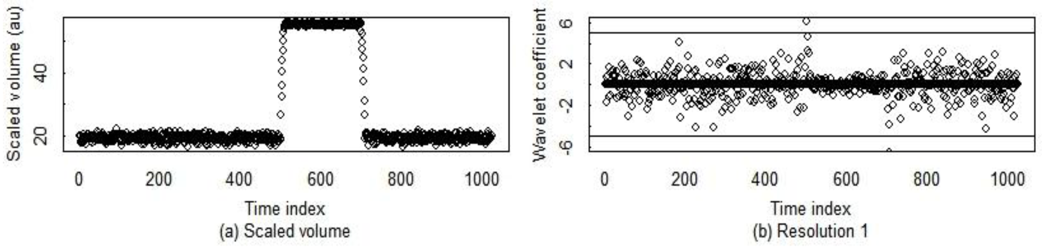
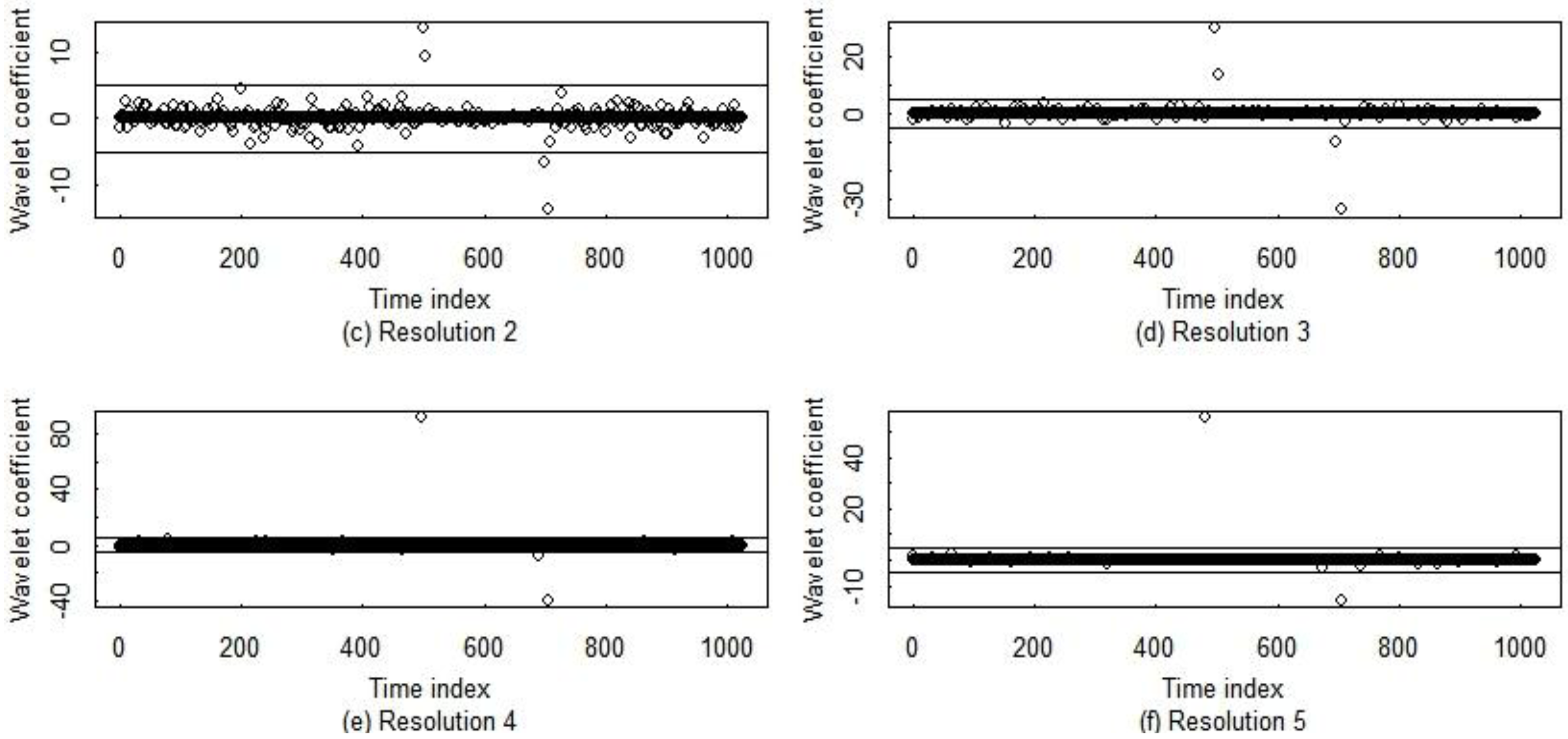
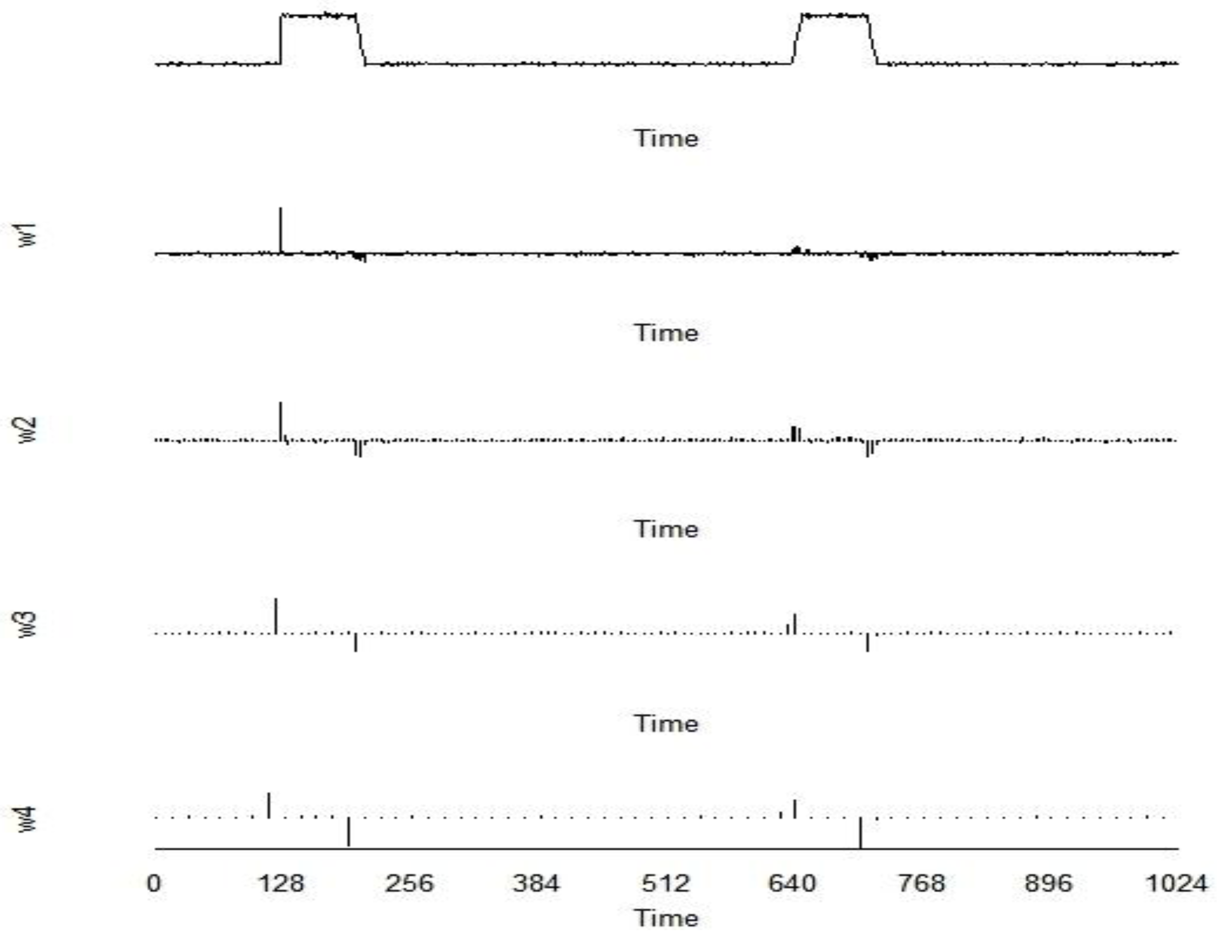
Axioms 02 00271 g005
Similarly, Figure 4 illustrates that standard multi-resolution wavelet-based change detection is not tuned to our SM application. For example, the resolution 1 and 2 wavelet coefficient plots show multiple change points occurring during the gradual shipment. Therefore, an approach such as that used in [15] or in the lag-one-differencing change detection option to concatenate contiguous change points (“sub-events”) into a single shipment event is needed. Fortunately, as we show below, wavelet-based change detection is highly effective for finding change point regions, which we then refine to an estimated start and stop time of, for example, the shipment in Figure 4.
To the best of our knowledge, wavelet literature assumes purely additive error models [12,27,28] rather than the combination of additive and multiplicative errors in Equation (1) that are more appropriate for SM data [10]. Therefore, we evaluated whether transforming to approximately unit variance prior to wavelet-based change detection was helpful. If the true value Tt at each time step t were known exactly, then rescaling M(t) by dividing by σ A 2 + T t 2 σ R 2 would convert the time series to a unit variance time series with purely additive error. Because 
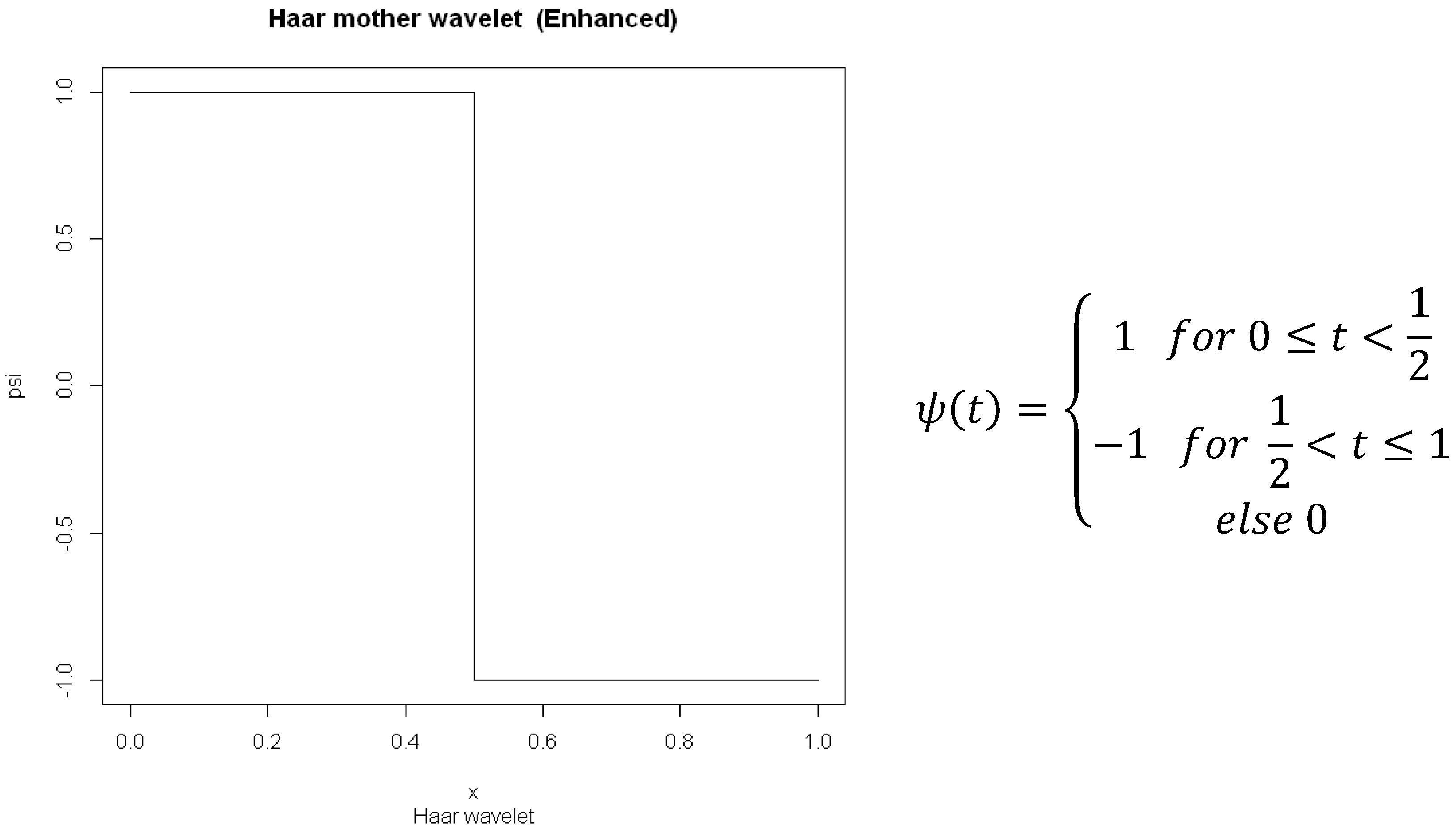
Tt is unknown, it must be estimated using T ^ t , which we obtained using an initial Haar-based wavelet transform. Because of estimation error in T ^ t the scaled M(t) has only approximately unit variance, and departures from unity tend to occur near the change points. All quantitative results are for the option that first scales M(t) to approximately unit variance prior to performing change detection; however, whether to transform the simulated SM data to approximately unit variance by first performing an initial smoothing made very little difference in the ability of Haar wavelets to find approximate change point regions.

4.2. Refining the Initial Estimate of the Time of Each Change Point

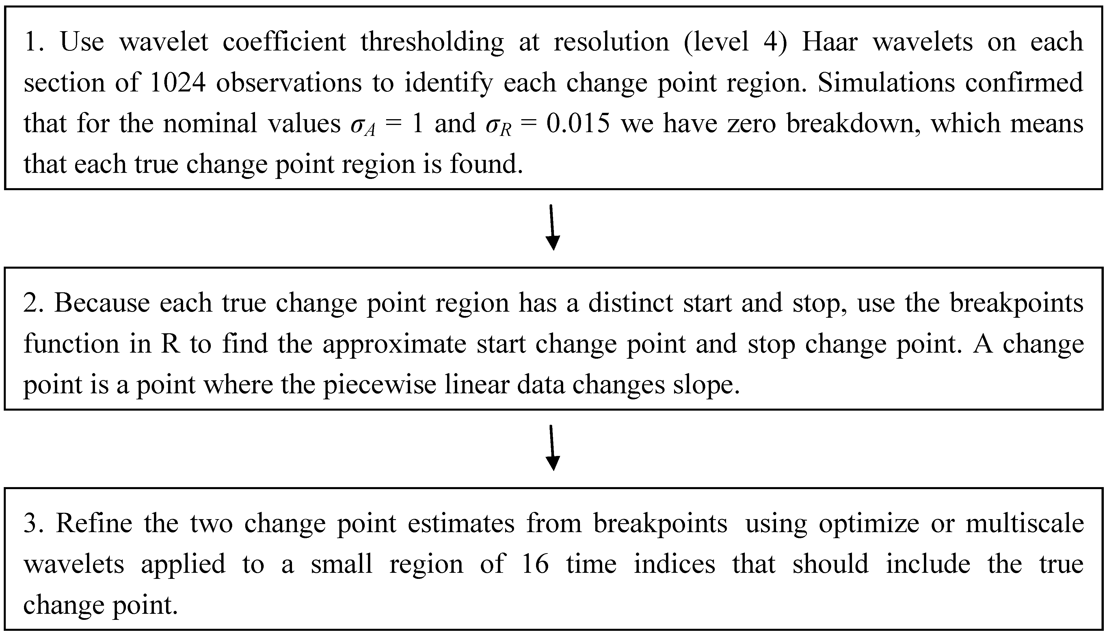
As discussed above, all methods we consider first locate an approximate change “region”. Then, because we anticipate a slope change in T(t) at the start and stop times of each change region, we apply breakpoints to find the approximate start and stop times of each change region, specifying to breakpoints that there are two change points in a small change region. Next, we refine the initial change point estimate. To do so, a simpler version of breakpoints that estimates only one change point at a time (see the Supplemental Information), suitable for data regions that are known to contain only one change point is applied near the estimated start time and near the estimated stop time. For comparison, a multi-scale wavelet option (see the Supplemental Information) is also applied to data regions that are known to contain only one change point. The multi-scale wavelet option applies wavelets only to the 16 time indices near each change point.
We summarize our change point detection approach in Section 4.1 and Section 4.2 with a block 3-step scheme as follows.
Axioms 02 00271 g008

4.3. Qualitative and Quantitative Simulation Results

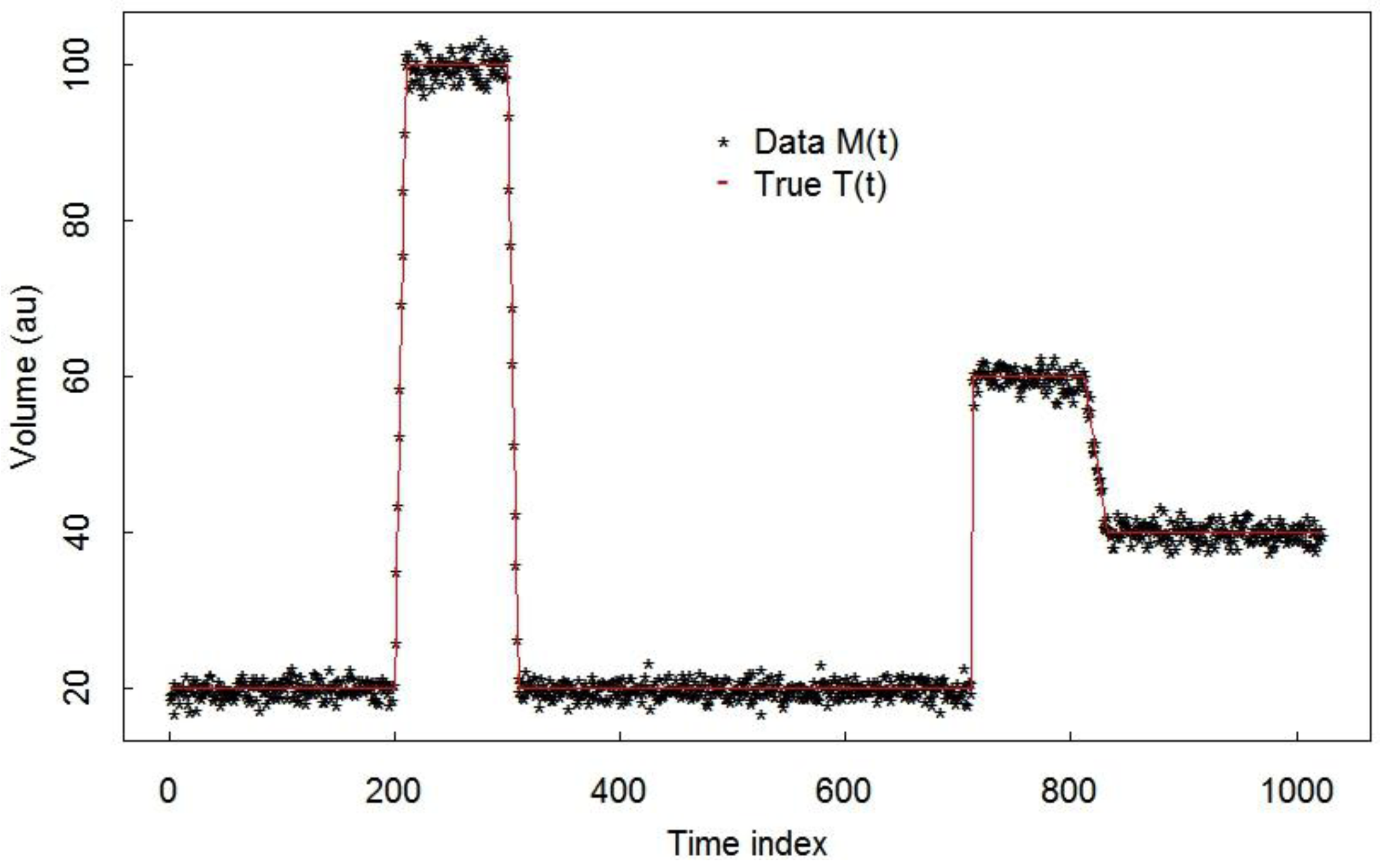
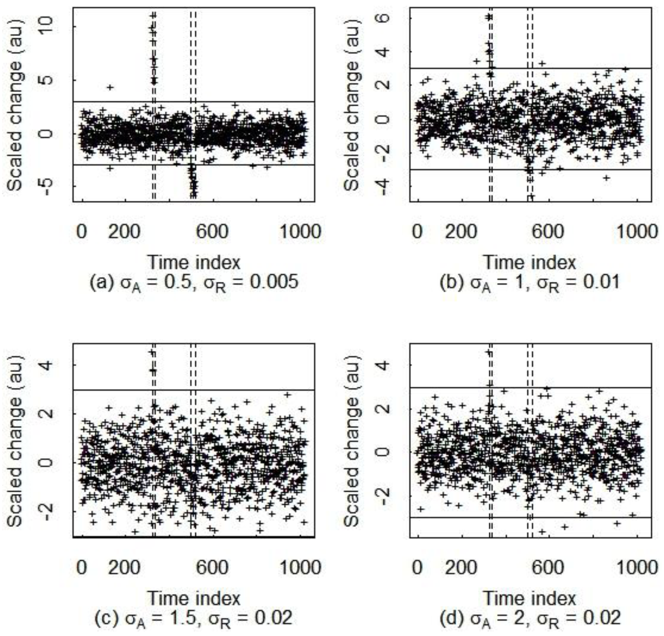
Figure 6 illustrates the lag-one differencing option for approximate change region detection for the gradual receipt and shipment in the first tank cycle in Figure 1. As σA and σR in Equation (1) increase in going from subplots (a) to (d) in Figure 6, the gradual receipt and shipment regions become very difficult to detect. Recall that 
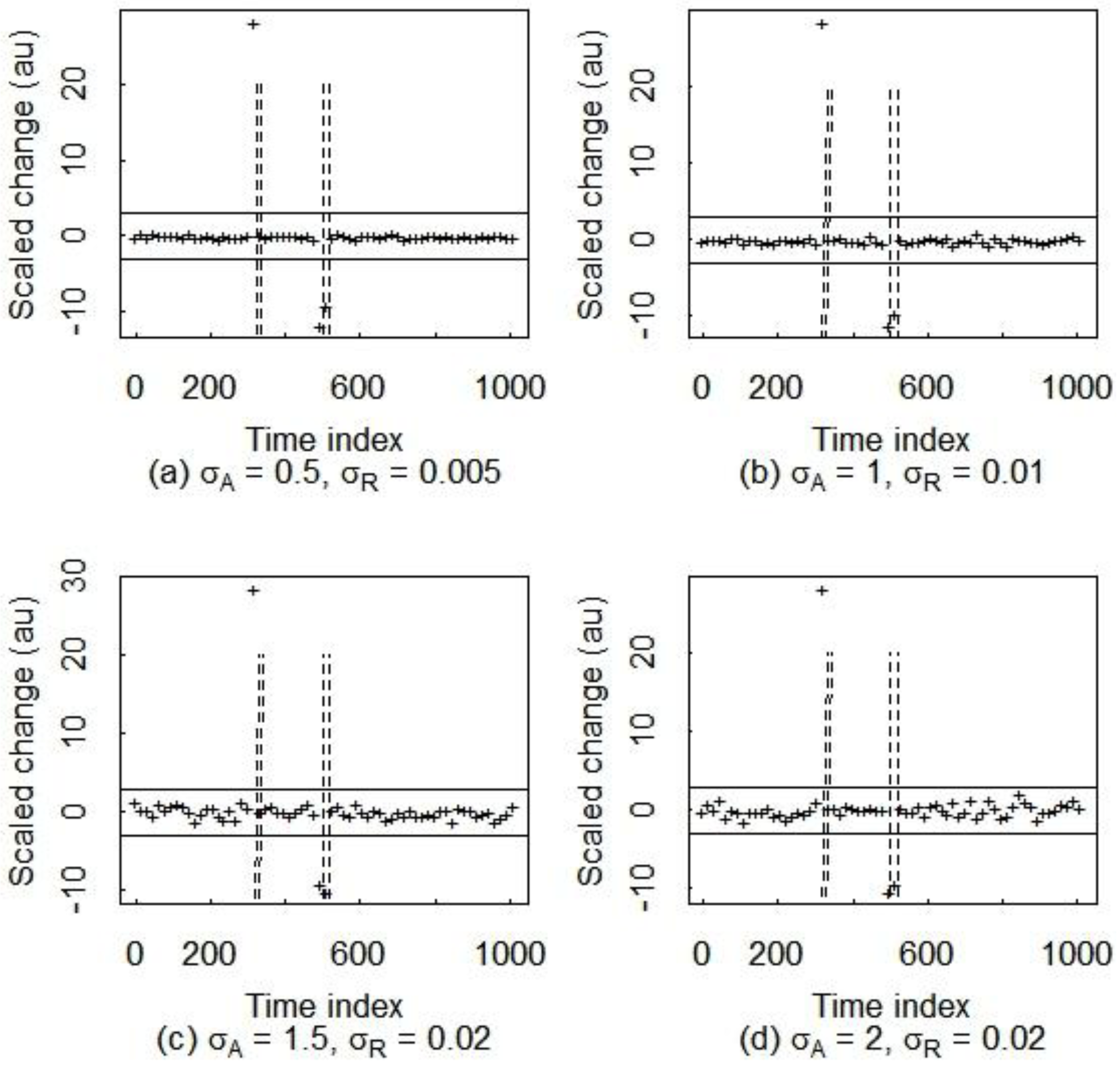
Figure 4 illustrated the potential of Haar-wavelet based change detection for a gradual receipt and gradual shipment. Comparing Figure 7 to Figure 6, note that Haar-wavelet based change region detection performs much better than the lag-one differencing. More quantitatively, using repeated sets of 1000 simulations of data as in Figure 3 with a gradual receipt and gradual shipment, we found that the breakdown σA and σR values (the σA and σR values at or above which the method to find each change region results in finding the wrong number of change regions) are approximately 1 and 0.03 for lag-one differencing and are approximately 8 and 0.12 for Haar-wavelet based change detection, which are both well above the values anticipated for our SM application. Of course the breakdown point depends on the rate of change of T(t) during each change region. But this example is representative of SM data, demonstrating a large advantage of a wavelet-based method to locate approximate change-point regions. We therefore have implemented Haar wavelet based change detection using high resolution to find approximate change point regions in sections of typically 512 or 1024 observations.
Figure 6. The scaled lag-one change for increasing values of σA and σR in Equation (1). Note that the abrupt shipment is easily detected but that the more gradual receipt is less easily detected. The two true change regions are indicated with vertical dashed lines. The values σA and σR in Equation (1) increase in going from subplots (a) to (d) in Figure 6, beginning with σA = 0.5 and σR = 0.005 in (a).
Axioms 02 00271 g006
Figure 7. The scaled change arising from the Haar-wavelet coefficient monitoring for increasing values of σA and σR in Equation (1) in subplots (ad). Note that both the gradual shipment and the gradual receipts are easily detected for (ad) as σA and σR increase. The two true change regions are indicated with vertical dashed lines.
Axioms 02 00271 g007
Table 1 lists the root mean squared errors (RMSEs) for the breakpoints method of the estimated change points (receipt start and stop and shipment start and stop) both without and with refinement by the “one change-point at a time” option using optimize and also for the multi-scale wavelet option mentioned in Section 4.2 (see the Supplemental Information). Recall that Haar-based wavelet change detection is used in all cases to first find the approximate location of each change point. The Table 1 entries were calculated using 1000 sets of simulations at nominal values of σA (1.0) and σR (0.015) for a tank cycle similar to that in Figure 1, with a gradual receipt and gradual shipment, both occurring over 10 time steps. We verified by repeating the set of 1000 simulations that the RMSEs are repeatable across sets of 104 simulations to within approximately ±0.01 or less.
Table 1. The root mean squared errors (RMSEs) for change point detection with and without refinement using the optimize function using 104 simulations.
EventBreakpoints without refinementOptimize to refineMulti-Scale wavelets to refine
Receipt Start1.00.140.83
Receipt Stop5.30.221.7
Ship Start3.90.231.0
Ship Stop2.00.150.81
The RMSEs in Table 1 are a good high level summary of performance in the 104 simulations. Notice that the optimize option leads to very good (low) RMSE and the multiscale wavelet option is also quite effective, without having been tuned to this change detection problem (see the Supplemental Information). Using optimize, the start of the receipt was estimated as t = 499, 500, or 501 (the true was 500 in all 104 simulations) with relative frequency 0.003, 0.995, and 0.002, respectively, so the RMSE is very small (0.14). The RMSE value of 1.7 for the receipt using multi-scale wavelets to refine the initial estimate from breakpoints can probably be reduced by more careful tuning of the multiscale wavelet approach (see the Supplemental Information). Estimation behavior without and with refinement was similar for the shipment. Qualitatively, we expect lower RMSE at the start of the receipt and at the end of the shipment because relative errors have smaller impact at the lower volumes.
Because refinement using optimize is simple and has slightly better performance than refinement using our implementation of multi-scale wavelets, we recommend Haar-based wavelets with resolution 4 to find each change point region. Certainly, we might find a multi-scale wavelet option that is more tuned to this type of SM that bundles together steps one and two. However, it is known that the change point location initial estimate will need some type of refinement [15,23]. For example, we verified by simulation that varying the location of the change point relative to the data length and/or changing the parity of the change point location [29] leads to additional variation between the estimated and true change point location. In addition, the Supplemental Information gives a numerical example of noise in the estimated change point location using multi-scale wavelets. Future work will consider in more detail whether there are performance or implementation advantages to using a “purely wavelet” based change detection.
To summarize this section, Haar-based wavelet change detection with resolution level 4 as in Figure 4 has the best breakdown and so is recommended for finding the approximate location of each change point region. Then, a very simple application of breakpoints to find the start and stop of each change region, or optimize (our preference) to refine the initial estimate of each change point within the change region completes the procedure. Figure 5 illustrates the excellent performance (high breakdown of Haar-based wavelet change region detection). Table 1 summarizes the RMSEs with and without either the optimize-based or the multi-scale-wavelet-based refinement step.

5. Conclusion

It is important to find change points in solution monitoring (SM) data because change points identify gain or loss of nuclear material, and are used to detect any undeclared losses. It is known that wavelet change detection as well as other change detection options can identify the location of change points, but of course any method’s performance will suffer as the signal-to-noise ratio decreases.
One simplifying feature of our SM application is that change regions each have a start and stop index describing a receipt or a shipment. Because the wavelet coefficients wjk approximately follow a known distribution that can be assessed using simulation as we did, a simple outlier test can identify the wjk associated with change regions. Haar wavelets performed extremely well at finding change regions, much better, for example, than the lag-one-differencing option in terms of breakdown, which is the additive and relative error standard deviation at or above which the method fails to find the correct number of change regions. Therefore, all methods we consider first locate an approximate change “region” using wavelet coefficients. Then, we use breakpoints to find the approximate start and stop index in the change region and recommend refining the estimates from breakpoints by isolating each breakpoint and applying optimize as shown in the Supplemental Information. Another refinement method that uses multi-scale wavelets was also evaluated as shown in the Supplemental Information. Because of the excellent RMSE results resulting from using optimize to refine the initial estimates from breakpoints, we did not attempt to optimize the multi-scale wavelet refinement option, but leave such optimization to future work.
Future work will also investigate whether an approach that is based entirely on wavelets can be better tuned for our application that has good breakdown and low RMSE. However, the performance of Haar-based wavelets to find approximate change point regions followed by the very simple application of optimize to refine the initial estimate of each change location is excellent so is our current recommendation. Qualitatively, our key summary is Figure 7 where both the gradual shipment and the gradual receipts are easily detected for a wide range of σA and σR in Equation (1). Quantitatively, our key summary is the RMSEs in Table 1 where refinement of the each change point location initial estimate reduces the RMSEs.

Conflict of Interest

The authors declare no conflict of interest.

References

  1. Burr, T.; Longo, C. Gibbs phenomenon in wavelet analysis of solution monitoring data for nuclear safeguards. Axioms 2013, 2, 44–57. [Google Scholar] [CrossRef]
  2. Wang, Y. Jump and sharp cusp detection by wavelets. Biometrika 1995, 82, 385–397. [Google Scholar] [CrossRef]
  3. Tang, Y. Wavelet Theory and Its Application to Pattern Recognition; World Scientific: New Jersey, NJ, USA, 2000. [Google Scholar]
  4. Burr, T.; Hamada, M.; Skurikhin, M.; Weaver, B. Pattern recognition options to combine process monitoring and material accounting data in nuclear safeguards. Stat. Res. Lett. 2012, 1, 6–31. [Google Scholar]
  5. Burr, T.; Howell, J.; Suzuki, M.; Crawford, J.; Williams, T. Evaluation of Loss Detection Methods in Solution Monitoring for Nuclear Safeguards. In Proceedings of American Nuclear Society Conference on Human-Machine Interfaces, Knoxville, TN, USA, 5–9 April 2009.
  6. Suzuki, M.; Hori, M.; Nagaoka, S.; Kimura, T. A study on loss detection algorithms using tank monitoring data. J. Nucl. Sci. Technol. 2009, 46, 184–192. [Google Scholar] [CrossRef]
  7. Burr, T.; Suzuki, M.; Howell, J.; Hamada, M.; Longo, C. Signal estimation and change detection in tank data for nuclear safeguards. Nucl. Instrum. Methods Phys. Res. A 2011, 640, 200–221. [Google Scholar] [CrossRef]
  8. Burr, T.; Suzuki, M.; Howell, J.; Hamada, M. Loss detection results on simulated tank data modified by realistic effects. J. Nucl. Sci. Technol. 2012, 49, 209–221. [Google Scholar] [CrossRef]
  9. Aigner, H.; Binner, R.; Kuhn, E. International target values 2000 for measurement uncertainties in safeguarding nuclear materials. Available online: http://www.inmm.org/topics/publications (accessed on 3 March 2012).
  10. Binner, R.; Howell, J.; Jahssens-Maenhous, G.; Sellinschegg, D.; Zhao, K. Practical issues relating to tank volume determination. Ind. Eng. Chem. Res. 2008, 47, 1533–1545. [Google Scholar] [CrossRef]
  11. Howell, J. Towards the re-verification of process tank calibrations. Trans. Inst. Meas. Control 2009, 31, 117–128. [Google Scholar] [CrossRef]
  12. Donoho, D.; Johnstone, I. Adapting to unknown smoothing via wavelet shrinkage. J. Am. Stat. Assoc. 1995, 90, 1200–1224. [Google Scholar] [CrossRef]
  13. Bakshi, B. Multiscale analysis and modeling using wavelets. J. Chem. 1999, 13, 415–434. [Google Scholar] [CrossRef]
  14. Nason, G.P. Wavelet Methods in Statistics with R; Springer: New York, NY, USA, 2008. [Google Scholar]
  15. Mihcak, K.; Kozintsev, I.; Ramchandran, K.; Moulin, P. Low-complexity image denoising based on statistical modeling of wavelet coefficients. IEEE Signal Process. Lett. 1999, 6, 300–303. [Google Scholar] [CrossRef]
  16. Sharifazadeh, M.; Azmoodeh, F.; Shahabi, C. Change detection in time series data using wavelet footprints. In Proceedings of Symposium on Large Spatial Databases, Angra dos Reis, Brazil, 22–24 August 2005; Medeiros, C.B., Egenhofer, M.J., Bertino, E., Eds.; Springer: Heidelberg, Germany, 2005; pp. 127–144. [Google Scholar]
  17. Mallat, S.; Hwang, L. Singularity detection and processing with wavelets. IEEE Trans. Inf. Theory 1992, 38, 617–643. [Google Scholar] [CrossRef]
  18. Mallat, S.G. A Wavelet Tour of Signal Processing, 2nd ed.; Elsevier: Boston, MA, USA, 1999. [Google Scholar]
  19. Lam, E. Statistical modelling of the wavelet coefficients with different bases and decomposition levels. IEEE Image Signal Process. 2004, 151, 203–206. [Google Scholar] [CrossRef]
  20. Antoniadis, A.; Gijbels, I. Detecting abrupt changes by wavelet methods. J. Nonparametr. Stat. 1997, 14, 7–29. [Google Scholar] [CrossRef]
  21. Bai, J.; Perron, P. Computation and analysis of multiple structural change models. J. Appl. Econom. 2003, 18, 1–22. [Google Scholar] [CrossRef]
  22. Raimondo, M.; Nader, T. A peaks over threshold model for change-point detection by wavelets. Stat. Sin. 2004, 14, 395–412. [Google Scholar]
  23. Canny, J. A computational approach to edge detection. IEEE Trans. Pattern Anal. Mach. Intell. 1986, 8, 679–698. [Google Scholar] [CrossRef] [PubMed]
  24. Daubechies, I. Ten Lectures on Wavelets; Society for Industrial and Applied Mathematics: Philadelphia, PA, USA, 1992. [Google Scholar]
  25. Vidakovic, B.; Lozoya, C. On time-dependent wavelet denoising. IEEE Signal Process. 1998, 46, 2549–2554. [Google Scholar] [CrossRef]
  26. R Statistical Programming Language. Available online: www.r-project.org (accessed on 7 July 2007).
  27. Donoho, D.; Johnstone, I. Ideal spatial adaption by wavelet shrinkage. Biometrika 1994, 81, 425–455. [Google Scholar] [CrossRef]
  28. Johnstone, I.; Silverman, B. Wavelet threshold estimators for data with correlated noise. J. R Stat. Soc. B 1997, 59, 319–351. [Google Scholar] [CrossRef]
  29. Xiaohong, G.; Jinhui, C. Study of the Gibbs phenomenon in de-noising by wavelets. In Proceedings of the 7th World Congress on Intelligent Control and Automation, Chongqing, China, 25–27 June 2008.

