Abstract
This paper is devoted to the study of the existence and uniqueness of solutions for a class of differential problems previously investigated by Laadjal. Our main contribution lies in deriving sharper estimates for the associated Green’s functions and employing Rus’s fixed-point theorem within a suitably defined metric framework. Notably, the conditions under which our results hold are less restrictive, thereby encompassing a wider class of problems for which the existence and uniqueness of solutions can be rigorously guaranteed. This theoretical advancement is supported by numerical evidence presented in the final stage of our analysis. A key strength of the proposed approach is that it does not rely on stringent contraction conditions, which enhances its potential applicability to more general classes of fractional differential systems.
Keywords:
fractional calculus; boundary value problems; Rus’s fixed-point theorem; nonlinear equations; numerical comparison MSC:
34A08; 47H10
1. Introduction
The mathematical modeling of real-world phenomena has increasingly turned to fractional-order differential equations, owing to their ability to capture memory and hereditary properties inherent in various natural and engineering processes. These equations have found impactful applications across a range of disciplines, including but not limited to control systems, biological processes, physical sciences, electrical circuit theory, wave dynamics, hemodynamics, and the fields of signal and image analysis. Readers seeking a deeper insight into the breadth of these applications may consult [1,2,3,4,5,6,7,8] and the sources cited therein.
One central aspect in the study of such equations is the investigation of solution existence and uniqueness. This issue is not only pivotal for fractional-order models but also mirrors classical concerns in the analysis of integer-order differential equations. A broad spectrum of results addressing these issues—primarily through the use of fixed-point theory—can be found in the literature; see, for instance, ref. [9] and the references therein.
Among the various analytical techniques developed in this context, particular attention has recently been given to approaches leveraging the extremal properties of Green’s functions associated with the integral form of the problem. This methodology, while offering refined estimates and analytical precision, has only been sparsely explored in the existing body of work. Given the limited number of studies on this topic, we refer the reader to these few existing contributions identified during our literature review for a more in-depth insight into the sufficient conditions for the existence and uniqueness of solutions to fractional boundary value problems (FBVP).
To avoid unnecessary repetition, we forgo an extensive literature review and instead turn directly to the objectives of this work. This article specifically analyzes the existence and uniqueness of the solutions to the following FBVPs
where represents the Riemann–Liouville fractional derivative of order q, belongs to the set of continuous real-valued functions defined on , which we refer to as , and .
Problem (1) was recently examined in a study by Laadjal [9], where the author established, in Theorem 2.3, an explicit sufficient condition for the existence and uniqueness of its solution. This result was obtained by combining an exact calculation of the maximum value of the integral of the Green function with an application of the Banach fixed-point theorem.
Of particular relevance is the fact that Almuthaybiri, S. and Tisdell, C. [10,11] were among the first to introduce Rus’s fixed-point theorem into the study of boundary value problems. The technique developed in their work provided a more adaptable framework than traditional fixed-point tools such as Banach’s theorem, particularly by weakening the required Lipschitz conditions while still guaranteeing solution existence and uniqueness. Following this, Rus’s theorem has been employed to analyze fractional boundary value problems involving Caputo, Riemann–Liouville, and conformable fractional derivatives [12,13,14]; see also [15,16,17,18,19,20].
Building upon these recent advancements, this study concentrates on the Riemann–Liouville fractional derivative of order In particular, we aim to extend and refine the results previously established by Laadjal in [9]. The cornerstone of this refinement lies in deriving new, sharper bounds for specific integrals involving the Green’s function introduced in [9]. These enhanced estimates are subsequently applied to an FBVP, analyzed within a function space equipped with two distinct metrics. To guarantee the existence and uniqueness of solutions, we employ Rus’s fixed-point theorem [21], a framework that provides a more general and adaptable alternative to classical fixed-point techniques. This approach not only broadens the scope of problems that can be addressed but also relaxes certain restrictive conditions inherent in traditional methods, thereby enhancing its applicability to a wider range of fractional differential equations.
The structure of this research is as follows. In Section 2, we introduce the fundamental notations, essential definitions, and theoretical tools that form the basis of our analysis. Section 3 presents new properties of the Green’s function, which serve as essential analytical tools in the subsequent development of our study. Section 4 is devoted to deriving novel sufficient conditions that guarantee the existence and uniqueness of solutions to the considered FBVP. Section 5 presents a comparative analysis between our condition and that proposed by Laadjal [9].
2. Notations and Intermediate Results
This section lays the foundation for the analysis to come. We present the notational framework, formal definitions, and the main theoretical results supporting Rus’s contraction approach. Let us first invoke a recent result due to Zaidi and Almuthaybiri, presented as Theorem 4.5 in [22]. This theorem provides a crucial foundation for the computation of the -norm of the Green function, which will be carried out in the next section.
For clarity, we define the following symbols and conventions:
- refers to the set of non-negative integers, to the set of all integers, to the real numbers, and to the complex numbers.
- stands for the real part of a complex number z.
The following is the definition of the Gauss hypergeometric function
Definition 1.
([23]). The Gauss hypergeometric function, denoted by , is defined by the following power series:
where the parameters satisfy:
Here, denotes the Pochhammer symbol defined for any and by:
If , then the value of the Gauss hypergeometric function at is given by the classical identity:
In addition, it is well known (see [23,24]) that when the first parameter is a non-positive integer, specifically for , and the parameter does not take on non-positive integer values (i.e., ), the hypergeometric series terminates after a finite number of terms. In this case, the function reduces to a polynomial of degree m:
where denotes the Pochhammer symbol.
Moreover, the Gauss hypergeometric function satisfies the following differentiation formula (see again [23,24]):
Finally, a natural generalization of the Gauss hypergeometric function is the function, defined by the series:
where the parameters satisfy:
As part of our discussion on the integration of the Green’s function in Section 3, we present the following recent result ([22], Theorem 4.5) by Zaidi and Almuthaybiri.
Theorem 1.
For all , and , we have
where,
Proof of Theorem 1.
The results stated in Theorem 1 follow directly from Theorem 4.5 of paper [22] upon making the substitutions , , , and . □
We proceed by presenting the following useful results, which are instrumental to the analysis carried out in the next sections. The following corollary was presented in ([22], Corollary 3.1), which gives explicit an expression for the hypergeometric function . This expression plays a crucial role in deriving a specific integral estimate involving the Green’s function.
Corollary 1.
We have
Proof of Corollary 1.
Equality (9) follows directly from Corollary 3.1 in paper [22], where a detailed proof is presented. □
The following Lemma will be important for our analysis in Section 3. The proof of this Lemma follows similar reasoning to that of ([12], Lemma 1).
Lemma 1.
Let and . Define
Then, is strictly decreasing on the interval and satisfies
Proof of Lemma 1.
The proof is separated into two cases according to the value of q.
First case: . Applying relation (6) for the derivative of the hypergeometric function with parameters , , and , we obtain
Given that the hypergeometric function has strictly positive coefficients in its series representation and converges for , one can deduce that
Since , then for all and is strictly decreasing on .
This simplified form of the function shows that it is strictly decreasing on the interval . Hence, is a strictly decreasing function on for all .
On the other hand, the function is well defined and analytic on , as its hypergeometric series converges for all . Therefore,
- using the monotone limit theorem and the monotonicity of (see [25], Theorem 3.3.15), we obtain
- using Relation (4), we obtain
This completes the proof of this lemma. □
Remark 1.
Let as defined in Theorem 1. By Lemma 1, since
we have
Remark 2
(See Remark 1 in [12]; see also [13]). It should be noted that the identity in (7) appears to have been available as a specific case of a more general result available in earlier work [24] (Relation (2.46), p. 41). We respectfully acknowledge this prior contribution.
The theorem below, originally established by Rus, serves as a fundamental tool in our analysis, which aims to refine the conditions previously proposed by Laadjal [9]. For recent advancements and applications of Rus’s theorem, the reader may consult [10,11,12,13,15].
Theorem 2
(Rus [21]). Let be a non-empty set and ρ and σ be two metrics on such that forms a complete metric space. If the following conditions are satisfied,
- (1)
- the mapping is continuous on the metric space ,
- (2)
- such that , for all ,
- (3)
- such that , for all .
Then, there exists a unique such that .
It is important to observe that Rus’s fixed-point theorem is formulated in the setting of two metrics, with completeness required only for the first. More precisely, the theorem assumes that the space is complete with respect to but not necessarily with respect to . The operator T is required to be continuous in the metric and contractive in the metric , while contractiveness with respect to is not imposed. Such assumptions, as will be shown, are particularly useful when dealing with operators associated with boundary FBVP, since they refine classical results by establishing uniqueness for a broader class of problems. As the analysis proceeds, we introduce the space , the metrics and , the operator T, and the constants and .
Let us consider the function space introduced earlier. To quantify the difference between two functions in this space, we introduce two metrics. The first is the uniform (or ) distance, denoted by , defined as
The second is the distance, denoted , defined by
These two distances yield different completeness properties. The space is complete (see [26], Corollary 4.11, p. 60). On the other hand, is not complete (see [26], p. 89). Furthermore, for any two functions , the following inequality holds:
3. New Properties of the Green’s Function
This section establishes two key results related to the integration of the Green’s function. These results serve as a foundation for the subsequent section, in which we formulate a new sufficient condition ensuring the existence and uniqueness of solutions to the FBVP (1).
In [9], Lemma 2.1, Laadjal proves that if , then the solution of the FBVP (1) is given by the integral equation
where is the set of measurable real-valued functions defined on the closed interval and is the following Green function
Lemma 2.
For all , the Green’s function exhibits the following relations:
where,
Proof of Lemma 2.
where denotes the integral given by (7). In light of Remark 1, we have Thus, we have:
that is,
and this achieves the proof of the first point of Lemma 2.
Let and C denote the function and constant defined below, respectively,
From the expression of the Green function (21), we deduce that for all , we have
and that for all , we have
- (1)
- For all we have
- (2)
- From relation (25) above, we have
4. A Refined Sufficient Condition Ensuring the Existence and Uniqueness of the Solution to Problem (1)
This section is devoted to establishing new sufficient conditions that guarantee the existence and uniqueness of solutions to the fractional boundary value problem (1). This condition is formally stated in the theorem below.
Theorem 3.
Proof of Theorem 3.
Utilizing the integral formulation (20) of the fractional boundary value problem (1), we define an operator T on the space , where each function is mapped to as follows
To establish the existence and uniqueness of a fixed point for the operator T, we invoke Rus’s Theorem 2.
- Verification of condition (1) in Theorem 2: Consider metrics distance and distance on the set . Then, for all , , we have
Note that we used Hölder’s inequality [27,28] and relation (29) to derive inequality (32) and used relation (22) to obtain inequality (33).
Let be the constant defined as follows
Since relation (33) is true for all , then
From the combination of inequalities (35) and (19), it follows that the subsequent bound holds for all functions
Relation (36) expresses the Lipschitz continuity of the mapping T on the metric space .
Expressing assumption (30) of Theorem 3 using , we immediately obtain the condition . We have thus proven that there exists a constant such that for all . Consequently, condition (3) of Rus’s theorem is fulfilled.
Since all the conditions of Theorem 2 are satisfied, it follows that the operator T possesses a unique fixed point. Accordingly, for any , the fractional boundary value problem (1) admits a unique solution . This concludes the proof of Theorem 3. □
Examination of FBVP for the Specific Case
When , then FBVP (1) is rewritten as follows
This special case was also examined by Laadjal [9]. More precisely, he demonstrated in Corollary 2.4
that problem (42) has a unique solution provided that the condition
is satisfied.
We now proceed to examine the sufficient condition for existence and uniqueness that arises from our approach, which is grounded in Rus’s fixed-point theorem.
By setting , Lemma 2 simplifies to the following corollary, which can be derived through direct integration.
Corollary 2.
When , the Green’s function exhibits the following relations:
By employing the same methodology used in the proof of Theorem 3, we derive the condition stated in Corollary 3 below.
Corollary 3.
Let K be a positive constant and be a continuous K-Lipschitz function with respect to its second variable u, that is, for all , it satisfies
Proof of Corollary 3.
Proceeding in the same manner as in the proof of Theorem 3, it follows that the contraction constant , defined by relation (40), can be expressed as
Therefore, the contraction condition (30) presented in Theorem 3 can be reformulated as
□
Remark 3.
Given that , condition (47) can be reformulated as the following equivalent expression:
which mirrors the form (43) exhibited by Laadjal.
This result demonstrates that our condition is less restrictive than that proposed by Laadjal, as it enables the establishment of existence and uniqueness for a broader class of problems of type (42). The next section presents a numerical comparison of the two conditions as the parameter q varies over the open interval .
5. Numerical Simulations
The primary aim of this section is to illustrate, through concrete examples, that our condition (30) established in Theorem (3) is less restrictive than that formulated by Laadjal in [9], Theorem 2.3. Specifically, we show that there exists an infinite family of FBVPs for which the existence and uniqueness of solutions are ensured by Theorem 3, but not by that of Laadjal, formulated as follows
For the sake of simplicity, we introduce the functions and , defined by:
Under this setting, Laadjal’s existence and uniqueness condition (51), along with our proposed condition (30), can be equivalently reformulated as follows
Unless otherwise specified, we assume and throughout the remainder of this paper.
Figure 1 illustrates the behavior of the functions D and as functions of the parameter q over the open interval . The graphical representation provides insight into the variation in these expressions with respect to q, highlighting their respective growth trends.
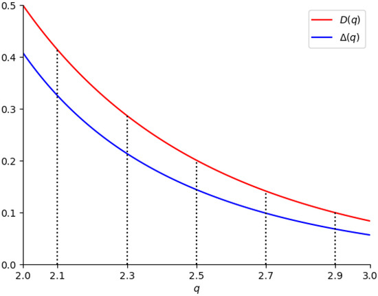
Figure 1.
Variation of and with respect to q over the interval .
In parallel, Table 1 lists the computed values of and for selected values of , rounded to five decimal places. This numerical data serves to complement the graphical analysis, offering concrete reference points for specific cases within the interval under consideration. The last row of this table reports the relative percentage deviation between and , which serves as a measure of the improvement achieved by our criterion in comparison with Laadjal’s condition.

Table 1.
Values of and for some special values of .
Consequently, Table 1 and Figure 1 provide clear visual evidence supporting the assertion that our condition represents a refinement of Laadjal’s criterion for ensuring existence and uniqueness.
In our computational framework, the functions and were implemented in Python 3 to generate Figure 1 and populate Table 1. The evaluation of the generalized hypergeometric function at unity was performed using the command hyper([1-q, 1, 2q], [q+1, 2q+1], 1).
To support our numerical results, we give an explicit fractional example to compare between our results and Laadjal’s result.
If , then (54) takes the form
Therefore,
Remark 4.
Interestingly, for , the explicit evaluations yield results identical to those obtained numerically.
5.1. Development of FBVP (1) Beyond Laadjal’s Condition
Let be a real parameter, and consider a continuous function that is L-Lipschitz continuous with respect to the variable u. As shown in Figure 1, the inequality holds for all . Thus, for any , we can define the function . It is straightforward to verify that g is continuous and satisfies a Lipschitz condition in u with constant . Under these conditions, the inequality is verified, while the condition is not. Therefore, applying Theorem 3, we conclude that FBVP (1), with and , admits a unique solution. On the other hand, Theorem 2.3 of Laadjal [9] does not prove the existence and uniqueness of the solution to this problem. This demonstrates that our condition represents a refinement over that of Laadjal, offering a stronger criterion for establishing the existence and uniqueness of solutions to problem (1).
5.2. Comparative Evaluation of the Two Criteria Through Concrete Examples
In both Laadjal’s Theorem 2.3 [9] and our Theorem 3, the continuity condition of the function is denoted by (a), while the Lipschitz condition of the function g with respect to the variable u is denoted by (b). This section provides illustrative examples, along with several others that can be derived from them, that satisfy conditions (a), (b), and (30) stated in Theorem 3. Notably, these examples do not fulfill condition (19) of Laadjal’s Theorem 2.3, thereby highlighting the broader applicability of our result.
5.2.1. Comparison of the Two Criteria When
Let us consider problem (1) in the specific case where and .
Recall that if the function is (a) continuous and (b) K-Lipschitzian with respect to the second variable u on the interval , then,
- according to our Theorem 3, Problem (60) admits a unique solution if
Here, conditions (a) and (b) are satisfied. Given that , condition (64) holds, while Condition (63) fails to be satisfied. This indicates that Laadjal’s criterion does not permit the conclusion of existence and uniqueness for the solution to Problem (60). Hence, our condition provides a sharper result than that of Laadjal.
5.2.2. Generating an Infinite Number of Counterexamples
As illustrated in Example (60), modifying the function to for various values of in the following interval
yields an infinite set of comparable examples, as we will show below.
Let . We define as the fractional boundary value problem derived from Problem (60) by substituting the function with :
Let , then is an L-Lipschitzian function with respect to u. Since
then
In this case as well, conditions (a) and (b) are satisfied. Furthermore, by combining inequalities (66) and (67), it follows that condition (64) is fulfilled, whereas condition (63) is not. This demonstrates that Laadjal’s criterion fails to guarantee the existence and uniqueness of a solution to Problem .
We have therefore constructed an infinite family of problems whose solvability—in terms of both existence and uniqueness—is ensured by Theorem 3, whereas Laadjal’s Theorem [9] fails to establish such a conclusion. This highlights the broader applicability and refinement of our result.
5.2.3. Comparison of the Two Criteria as
We now consider the problem presented in Example 2.7 of [9], modifying the fractional order from to and adjusting the study interval from to . This problem can be formulated as follows:
The function satisfies two fundamental properties: (a) it is continuous, and (b) it is K-Lipschitz continuous with respect to the variable u, where the Lipschitz constant is given by . Therefore,
- according to our Theorem 3, Problem (68) admits a unique solution if
From Table 1, and . By substituting the values of K, , and into the left-hand sides of conditions (69) and (70), we obtain
In accordance with our criterion, Problem (68) admits a unique solution, whereas Laadjal’s criterion does not permit such a conclusion. Hence, our condition provides a sharper result than that of Laadjal.
5.2.4. Comparison of the Two Criteria When
Let us consider problem (42) in the specific case where and :
Since , then we have:
In accordance with our criterion, Problem (72) admits a unique solution, whereas Laadjal’s criterion does not permit such a conclusion. Hence, our condition provides a sharper result than that of Laadjal.
Figure 2 illustrates the solution to Problem (72) for the two cases and . The computations were performed using the bvp4c routine in Matlab, which is specifically designed for the numerical resolution of boundary value problems. This solver is based on a collocation method, employing the three-stage Lobatto IIIa formula [29,30], a fourth-order finite difference scheme that ensures both accuracy and stability in the approximation of solutions.
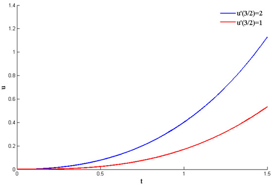
Figure 2.
The blue (resp. red) curve is the solution to problem (72) when (resp. ).
6. Conclusions
The first main result of this study, Theorem 3, was established for a specific choice of the distances and used by Rus’s fixed-point theorem. The rationale behind this choice lies in the feasibility of performing the integral computations required in Lemma 2. However, the left-hand side of relation (23) still lacks an explicit expression whenever with , and the task of obtaining a reliable numerical evaluation continues to pose a complex and unsolved problem.
By employing the new integral bounds for the Green functions associated with FBVP (1), derived in Section 3 for all , and applying Rus’s fixed-point theorem (Theorem 2), we established our main existence and uniqueness result, Theorem 3. This theorem provides sharper a priori bounds than those obtained via classical contraction methods and extends the earlier results of [9]. The validity of our findings is further supported by numerical comparisons.
However, it remains an open question whether alternative choices of the distances and , together with newly derived integral bounds for the Green functions of FBVP (1), could yield results that are even more robust than those presented here. In addition, it is of particular interest to investigate whether Rus’s fixed-point theorem constitutes a more effective alternative to the classical Banach fixed-point approach in addressing FBVP (1) for under suitable boundary conditions. These considerations suggest promising directions for future research.
Another avenue for future research could investigate the use of Rus’s fixed-point theorem in mathematical control theory, such as approximate controllability [31], and apply it to problems studied using recent fixed-point results in generalized metric spaces [32]. This approach may offer a promising framework for advancing the analysis of fractional boundary value problems and related applications.
Author Contributions
Conceptualization, S.S.A. and A.Z.; methodology, S.S.A. and A.Z.; software, A.Z.; validation, S.S.A. and A.Z.; formal analysis, S.S.A. and A.Z.; investigation, S.S.A. and A.Z.; resources, S.S.A. and A.Z.; writing—original draft preparation, S.S.A.; writing—review and editing, S.S.A. and A.Z.; visualization, S.S.A. and A.Z.; funding acquisition, S.S.A. All authors have read and agreed to the published version of the manuscript.
Funding
This research received no external funding.
Data Availability Statement
The original contributions presented in this study are included in the article. Further inquiries can be directed to the corresponding author.
Acknowledgments
The researchers would like to thank the Deanship of Graduate Studies and Scientific Research at Qassim University for financial support (QU-APC-2025).
Conflicts of Interest
The authors declares no conflicts of interest.
Correction Statement
This article has been republished with a minor correction to the Data Availability Statement. This change does not affect the scientific content of the article.
References
- Xiao, R.; Sun, H.; Chen, W. A finite deformation fractional viscoplastic model for the glass transition behavior of amorphous polymers. Int. J. Non-Linear Mech. 2017, 93, 7–14. [Google Scholar] [CrossRef]
- Cai, W.; Chen, W.; Xu, W. Fractional modeling of Pasternak-type viscoelastic foundation. Mech. Time-Depend. Mater. 2017, 21, 119–131. [Google Scholar] [CrossRef]
- Srivastava, H.M. Diabetes and its Resulting Complications: Mathematical Modeling via Fractional Calculus. Public Health Open Access 2020, 4, 1–5. [Google Scholar] [CrossRef]
- Zhang, G.; Zhu, Y.; Liu, J.; Chen, Y. Image Segmentation Based on Fractional Differentiation and RSF Model. In Proceedings of the 13th ASME/IEEE International Conference on Mechatronic and Embedded Systems and Applications (MESA), 2017, Volume 9, International Design Engineering Technical Conferences and Computers and Information in Engineering Conference, Cleveland, OH, USA, 6–9 August 2017; Volume 9, p. V009T07A023. [Google Scholar] [CrossRef]
- Pandey, V.; Holm, S. Connecting the grain-shearing mechanism of wave propagation in marine sediments to fractional order wave equations. J. Acoust. Soc. Am. 2016, 140, 4225–4236. [Google Scholar] [CrossRef] [PubMed]
- Li, Z.; Wang, H.; Xiao, R.; Yang, S. A variable-order fractional differential equation model of shape memory polymers. Chaos Solitons Fractals 2017, 102, 473–485. [Google Scholar] [CrossRef]
- Pinto, C.M.; Carvalho, A.R. A latency fractional order model for HIV dynamics. J. Comput. Appl. Math. 2017, 312, 240–256. [Google Scholar] [CrossRef]
- Marinangeli, L.; Alijani, F.; HosseinNia, S. A Fractional-order Positive Position Feedback Compensator for Active Vibration Control. IFAC-PapersOnLine 2017, 50, 12809–12816. [Google Scholar] [CrossRef]
- Laadjal, Z. Sharp estimates for the unique solution for a class of fractional differential equations. Filomat 2023, 37, 435–441. [Google Scholar] [CrossRef]
- Almuthaybiri, S.; Tisdell, C.C. Sharper existence and uniqueness results for solutions to fourth-order boundary value problems and elastic beam analysis. Open Math. 2020, 18, 1006–1024. [Google Scholar] [CrossRef]
- Almuthaybiri, S.; Tisdell, C.C. Sharper Existence and Uniqueness Results for Solutions to Third-Order Boundary Value Problems. Math. Model. Anal. 2020, 25, 409–420. [Google Scholar] [CrossRef]
- Almuthaybiri, S.S.; Zaidi, A.; Tisdell, C.C. Enhanced Qualitative Understanding of Solutions to Fractional Boundary Value Problems via Alternative Fixed-Point Methods. Axioms 2025, 14, 592. [Google Scholar] [CrossRef]
- Almuthaybiri, S. Some results on existence and uniqueness of solutions for fractional boundary value problems. J. Math. Comput. Sci. 2026, 40, 405–414. [Google Scholar] [CrossRef]
- Almuthaybiri, S.S. On classical and sequential conformable fractional boundary value problems: New results via alternative fixed point method. AIMS Math. 2025, 10, 19280–19299. [Google Scholar] [CrossRef]
- Stinson, C.; Almuthaybiri, S.; Tisdell, C.C. A note regarding extensions of fixed point theorems involving two metrics via an analysis of iterated functions. ANZIAM J. 2019, 61, C15–C30. [Google Scholar] [CrossRef]
- Almuthaybiri, S.; Tisdell, C. Existence and uniqueness of solutions to third-order boundary value problems: Analysis in closed and bounded sets. Differ. Equ. Appl. 2020, 12, 291–312. [Google Scholar] [CrossRef]
- Khuddush, M.; Prasad, K.R.; Krushna, B.M.B. Bootstrapping and fixed point techniques for the existence of solutions to iterative nonlinear elliptic systems. J. Elliptic Parabol. Equ. 2025, 11, 297–322. [Google Scholar] [CrossRef]
- Smirnov, S. Existence of a unique solution for a third-order boundary value problem with nonlocal conditions of integral type. Nonlinear Anal. Model. Control 2021, 26, 914–927. [Google Scholar] [CrossRef]
- Madhubabu, B.; Sreedhar, N.; Prasad, K.R. The existence of solutions to higher-order differential equations with nonhomogeneous conditions. Lith. Math. J. 2024, 64, 53–66. [Google Scholar] [CrossRef]
- Harjani, J.; López, B.; Sadarangani, K. Existence of a unique mild solution to a fractional thermostat model via a Rus’s fixed point theorem. Fixed Point Theory 2025, 26, 539–552. [Google Scholar]
- Rus, I.A. On a fixed point theorem of Maia. Stud. Univ. Babeş-Bolyai Math. 1977, 22, 40–42. [Google Scholar]
- Zaidi, A.; Almuthaybiri, S. Explicit evaluations of subfamilies of the hypergeometric function 3F2(1) along with specific fractional integrals. AIMS Math. 2025, 10, 5731–5761. [Google Scholar] [CrossRef]
- Kilbas, A.A.; Srivastava, H.M.; Trujillo, J.J. Theory and Applications of Fractional Differential Equations, Volume 204 (North-Holland Mathematics Studies); Elsevier Science Inc.: Philadelphia, PA, USA, 2006. [Google Scholar]
- Samko, S.G.; Kilbas, A.A.; Marichev, O.I. Fractional Integrals and Derivatives; Gordon and Breach: London, UK, 1993. [Google Scholar]
- Sohrab, H.H. Basic Real Analysis, 2nd ed.; Birkhäuser/Springer: New York, NY, USA, 2014; p. xii+683. [Google Scholar] [CrossRef]
- Robinson, J. An Introduction to Functional Analysis; Cambridge University Press: Cambridge, UK, 2020. [Google Scholar]
- Hölder, O. Ueber einen Mittelwerthabsatz. Nachrichten Königl. Ges. Wiss. Georg-Augusts Göttingen 1889, 1889, 38–47. [Google Scholar]
- Rogers, L.J. An extension of a certain theorem in inequalities. Messenger Math. 1888, 17, 145–150. [Google Scholar]
- Jay, L.O. Lobatto Methods. In Encyclopedia of Applied and Computational Mathematics; Engquist, B., Ed.; Springer: Berlin/Heidelberg, Germany, 2015; pp. 817–826. [Google Scholar] [CrossRef]
- Gradzki, M.J. Application of the MATLAB bvp4c Solver in the Linear Stability Analysis of Some Magnetohydrodynamic Problems; The Institute of Geophysics, Polish Academy of Sciences: Warszawa, Poland, 2022. [Google Scholar]
- Guran, L.; Mitrović, Z.D.; Reddy, G.S.M.; Belhenniche, A.; Radenović, S. Applications of a Fixed Point Result for Solving Nonlinear Fractional and Integral Differential Equations. Fractal Fract. 2021, 5, 211. [Google Scholar] [CrossRef]
- Shukla, A.; Sukavanam, N. Interior approximate controllability of second-order semilinear control systems. Int. J. Control 2024, 97, 615–624. [Google Scholar] [CrossRef]
Disclaimer/Publisher’s Note: The statements, opinions and data contained in all publications are solely those of the individual author(s) and contributor(s) and not of MDPI and/or the editor(s). MDPI and/or the editor(s) disclaim responsibility for any injury to people or property resulting from any ideas, methods, instructions or products referred to in the content. |
© 2025 by the authors. Licensee MDPI, Basel, Switzerland. This article is an open access article distributed under the terms and conditions of the Creative Commons Attribution (CC BY) license (https://creativecommons.org/licenses/by/4.0/).