Article

A Note on Multi-Index Mittag-Leffler Functions and Parametric Laguerre-Type Exponentials

by
Hari Mohan Srivastava
1,2,3,4,5,6,*,
Diego Caratelli
7,8 and
Paolo Emilio Ricci
6
1
Department of Mathematics and Statistics, University of Victoria, Victoria, BC V8W 3R4, Canada
2
Department of Medical Research, China Medical University Hospital, China Medical University, Taichung 40402, Taiwan
3
Center for Converging Humanities, Kyung Hee University, 26 Kyungheedae-ro, Dongdaemun-gu, Seoul 02447, Republic of Korea
4
Department of Applied Mathematics, Chung Yuan Christian University, Chung-Li, Taoyuan City 20314, Taiwan
5
Department of Mathematics and Informatics, Azerbaijan University, 71 Jeyhun Hajibeyli Street, AZ1007 Baku, Azerbaijan
6
Mathematics Section, International Telematic University UniNettuno, 39 Corso Vittorio Emanuele II, I-00186 Rome, Italy
7
Department of Research and Development, The Antenna Company, 5656 AE Eindhoven, The Netherlands
8
Department of Electrical Engineering, Eindhoven University of Technology, 5600 MB Eindhoven, The Netherlands
*
Author to whom correspondence should be addressed.
Axioms 2025, 14(9), 705; https://doi.org/10.3390/axioms14090705
Submission received: 20 August 2025 / Revised: 15 September 2025 / Accepted: 16 September 2025 / Published: 18 September 2025
(This article belongs to the Special Issue Special Functions and Related Topics, 2nd Edition)

Abstract

This paper explores the eigenfunctions of specific Laguerre-type parametric operators to develop multi-parametric models, which are associated with a class of the generalized Mittag-Leffler type functions, for dynamical systems and population dynamics. By leveraging these multi-parametric approaches, we introduce new concepts in number theory, specifically those involving multi-parametric Bernoulli and Euler numbers, along with other related polynomials. Several numerical examples, which are generated by using the computer algebra program Mathematica© (Version 14.3), demonstrate the effectiveness of the models that we have presented and analyzed in this paper.

1. Introduction

The connection between Mittag-Leffler functions and hyper-Bessel functions has been highlighted in several papers (see, for example, [1,2,3,4,5,6]). Their importance in fractional calculus is clearly demonstrated in these and other papers. Several interesting applications using one-parameter Mittag-Leffler functions in the study of physical phenomena have recently been obtained in [7,8].
In this paper, we propose to show that a set of special multi-index Mittag-Leffler functions can be viewed as generalized exponentials with respect to suitable generalized Laguerre-type operators. The multi-index functions, which we consider here, are a very special case of those of the type given by
E ( α i ) , ( β i ) r ( t ) = k = 0 t k k ! i = 1 r Γ ( α i k + β i ) ( r : positive integer ) ,
which were considered by Paneva-Konovska (see [5,6]) by extending those studied by Prabhakar [9].
Assuming that α i = 1 and β i = m i + 1 ( i = 1 , 2 , , r ) , with positive integers m i , the above functions simply become of the following form:
E ( m i ) r ( t ) = k = 0 t k k ! i = 1 r ( k + m i ) ! .
In what follows, we will examine the Laguerre-type operators for the functions in (2), since similar results using fractional-type operators are more complex, as demonstrated in [10] with reference to population dynamics models.

2. Pseudo Versus True Exponential Functions

The pseudo-exponentials, which were considered by Mishra (see, for example, [11] (p. 168, Equation (5.11))) are defined as follows:
e m ( t ) = k = 0 t k k ! ( k + m ) ! .
They satisfy the following property:
D t e m ( t ) = e m + 1 ( t ) ,
which is similar to the exponential property but with the shifted parameter m.
Here, and what follows, we use the derivative symbol
D t = D = d d t .
In fact, the functions in (3) are a special case of the generalized Mittag-Leffler function, which was studied by Prabhakar [9], in its following Laguerre-type version:
E α , β γ L ( z ) = k = 0 ( γ ) k z k ( k ! ) 2 Γ ( α k + β ) ,
where ( γ ) k denotes the Pochhammer symbol
( γ ) 0 = 1 and ( γ ) k = γ ( γ + 1 ) ( γ + 2 ) ( γ + k 1 ) = Γ ( γ + k ) Γ ( γ ) ,
since
e ( z , m ) = E 1 , m + 1 1 L ( z ) .
We remark in passing that the functions in each of Equations (1)–(3), and indeed also many of those which were similarly considered in numerous studies of the Mittag-Leffler type functions (see, for details, [12]), are rather obvious special cases of the relatively more widely and more extensively studied Fox–Wright function Ψ q p with p numerator parameters and q denominator parameters (see [13,14,15]; see also [16] (p. 183)). As a matter of fact, in a recent survey-cum-expository paper [17], the interested reader will find a comprehensive and extensive analysis of various general families of Mittag-Leffler type functions and their associated operators of fractional calculus, some of which have their origin in the monumental works by Barnes [18] in 1906 and Wright [19] in 1940 (see also [20,21]). Some potentially useful developments, which concern the familiar Mittag-Leffler function itself (see [22]), may be found in (for example) [23,24,25].
It is worth noting here that the function in Equation (3) can easily be seen to behave like a true exponential function with respect to the Laguerre-type operator D t D + m D .
Indeed, the following result holds true.
Theorem 1. 
The function e m ( t ) defined in (3), with a positive integer m , is an eigenfunction of the operator:
D t D + m D ,
since, for every complex constant a , it results
( D t D + m D ) a e m ( t ) = a e m ( t ) .
Proof. 
In fact, we have
( D t D + m D ) k = 0 t k k ! ( k + m ) ! = D t k = 1 t k 1 ( k 1 ) ! ( k + m ) ! + m k = 1 t k 1 ( k 1 ) ! ( k + m ) ! = D k = 0 t k + 1 k ! ( k + m + 1 ) ! + m k = 0 t k k ! ( k + m + 1 ) ! = k = 0 ( k + 1 ) t k k ! ( k + m + 1 ) ! + m k = 0 t k k ! ( k + m + 1 ) ! = k = 0 ( k + m + 1 ) t k k ! ( k + m + 1 ) ! = k = 0 t k k ! ( k + m ) ! ,
which evidently completes the proof of Theorem 1. □
For brevity, we use the following notations for the Laguerre-type operators:
D L = D t D = D + t D 2 and D 2 L = D + 3 t D 2 + t 2 D 3 ,
and, in general,
D n L : = D t D t D t D = S ( n + 1 , 1 ) D + S ( n + 1 , 2 ) t D 2 + + S ( n + 1 , n + 1 ) t n D + t n + 1 ,
where S ( n , k ) denote the Stirling numbers of the second kind, which are defined by the following generating functions:
z n = k = 0 n S ( n , k ) z ( z 1 ) ( z k + 1 ) ,
( e z 1 ) k = k ! n = k S ( n , k ) z n n !
and
( 1 z ) ( 1 2 z ) ( 1 k z ) 1 = n = k S ( n , k ) z n k | z | < 1 k .
Using this notation, we now generalize the result of Theorem 1 to the case of r parameters, starting from the case r = 2 .

The Two-Parameter Case

We note that, upon putting m = m 1 , the operator (4) becomes
D [ t D + m 1 ] ,
and, by introducing a second parameter m 2 , it can be iterated in the following form:
D [ t D + m 1 ] [ t D + m 2 ] = D [ t D t t D t + ( m 1 + m 2 ) t D t + m 1 m 2 ] = D 2 L + ( m 1 + m 2 ) D L + m 1 m 2 D .
The following result holds true.
Theorem 2. 
The function e m 1 , m 2 ( t ) defined by
e m 1 , m 2 ( t ) = k = 0 t k k ! ( k + m 1 ) ! ( k + m 2 ) ! ,
where m 1 and m 2 are positive integers, is an eigenfunction of the operator:
D 2 L + ( m 1 + m 2 ) D L + m 1 m 2 D ,
since, for every complex constant a , it results
[ D 2 L + ( m 1 + m 2 ) D L + m 1 m 2 D ] a e m 1 , m 2 ( t ) = a e m 1 , m 2 ( t ) .
Proof. 
The assertion of Theorem 2 follows by a direct computation, which is similar to that used in the proof of Theorem 1. And, indeed, it was validated by means of Mathematica© (Version 14.3). □

3. The General Case

The procedure used in the two-parameter case can be iterated in general by
D [ t D + m 1 ] [ t D + m 2 ] [ t D + m r ] = D r L + ( m 1 + m 2 + + m r ) D ( r 1 ) L + + m 1 m 2 m r D .
Thus, we find a polynomial in the Laguerre-type operators whose coefficients are the elementary symmetric functions of the parameters, and the following result emerges, which extends those asserted by Theorems 1 and 2.
Theorem 3. 
The function e m 1 , m 2 , , m r ( t ) defined by
e m 1 , m 2 , , m r ( t ) = k = 0 t k k ! i = 1 r ( k + m i ) ! ,
where m 1 , m 2 , , m r are positive integers, is an eigenfunction of the operator:
c r D r L + c r 1 D ( r 1 ) L + c r 2 D ( r 2 ) L + + c 1 D L + c 0 D ,
with
c h = 1 h ! d h d x h i = 1 r ( x + m i ) x = 0 ( h = 0 , 1 , , r ) ,
that is,
c r = 1 , c r 1 = i = 1 r m i , c r 2 = i , j = 1 i j r m i m j , 1 p t 26 p t c r 3 = i , j , k = 1 i j k r m i m j m k , , c 0 = i = 1 r m i ,
since, for every complex constant a , it results
c r D r L + c r 1 D ( r 1 ) L + c r 2 D ( r 2 ) L + + c 1 D L + c 0 D a e m 1 , m 2 , , m r ( t ) = a e m 1 , m 2 , , m r ( t ) .
Proof. 
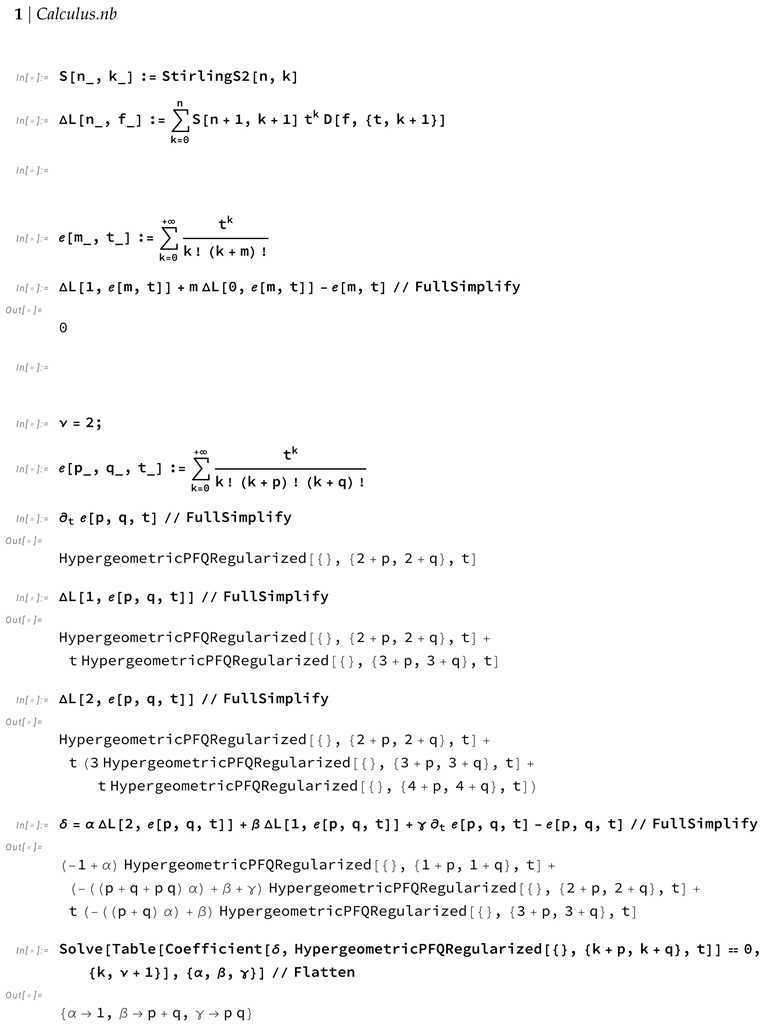
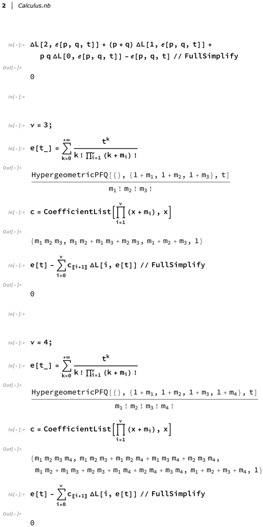
The proof of Theorem 3 can be developed by appealing to the principle of mathematical induction. The relevant verification was obtained up to the order r = 4 , using Mathematica© (Version 14.3), and can be found in Appendix A at the end of this article. □

4. Applications and Extensions

Regarding the possible applications of the multi-parameter functions introduced in the previous sections, we would like to emphasize that, since the exponential function is commonly used to model various physical phenomena and to define sequences of polynomials and special numbers, the introduction of the various forms of the above-mentioned multi-parametric exponentials can possibly be exploited to extend these phenomena and mathematical entities. This has been performed in the recent articles in special cases where generalizations of population dynamics have been illustrated (see [10,26], and the references therein), as well as definitions of new examples of polynomials and special numbers, which are studied in (for example) [27,28].

4.1. Multi-Parametric Linear Dynamical Systems

One of the standard applications of the exponential function is related to evolution problems. In this context, with reference to linear dynamical systems, an extension has already been made in [29], but broader generalizations can be obtained in the multi-parametric case. In order to be more precise, using the same technique applied in the above-cited recent work [29], it is possible to prove the following theorem.
Theorem 4. 
Let A = A r × r be an r × r non-singular complex matrix. Then the solution to the following Cauchy problem is
D r L + ( m 1 + m 2 + + m r ) D ( r 1 ) L + + m 1 m 2 m r D Z ( t ) = A · Z ( t ) Z ( 0 ) = Z 0 , Z ( 0 ) = C A · Z 0 = Z 0 , Z ( r ) ( 0 ) = C A r · Z 0 = Z 0 ( r ) ,
with
C = 1 c 0 + c 1 + + c r ,
is given by
Z ( t ) = k = 0 t k i = 1 r m i ! k ! i = 1 r ( k + m i ) ! α k ( A ) · Z 0 ,
where the coefficients satisfy the recursion formula:
α k ( A ) = A α k 1 ( A ) a n d α 0 ( A ) = I .
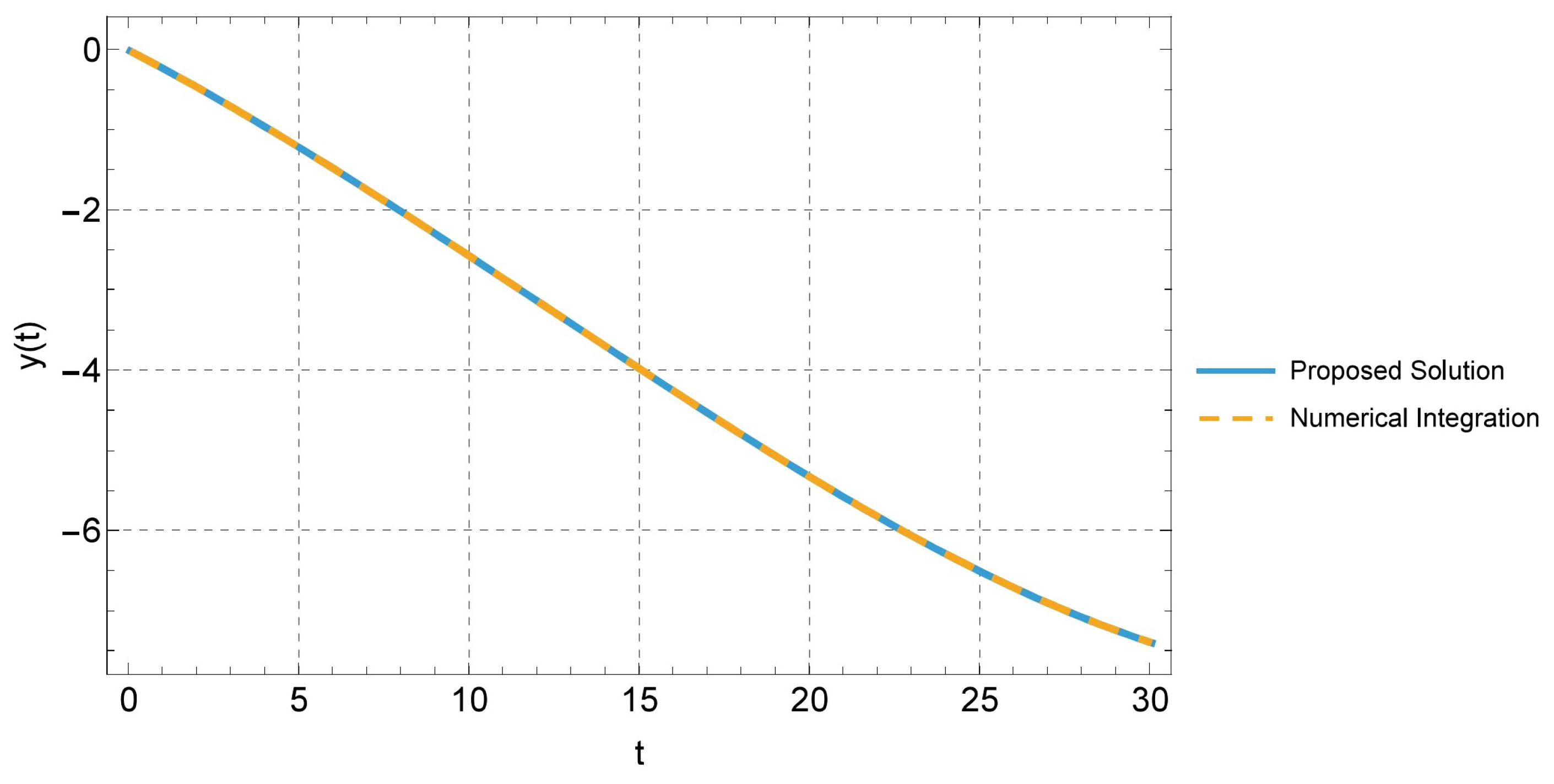
Example 1. 
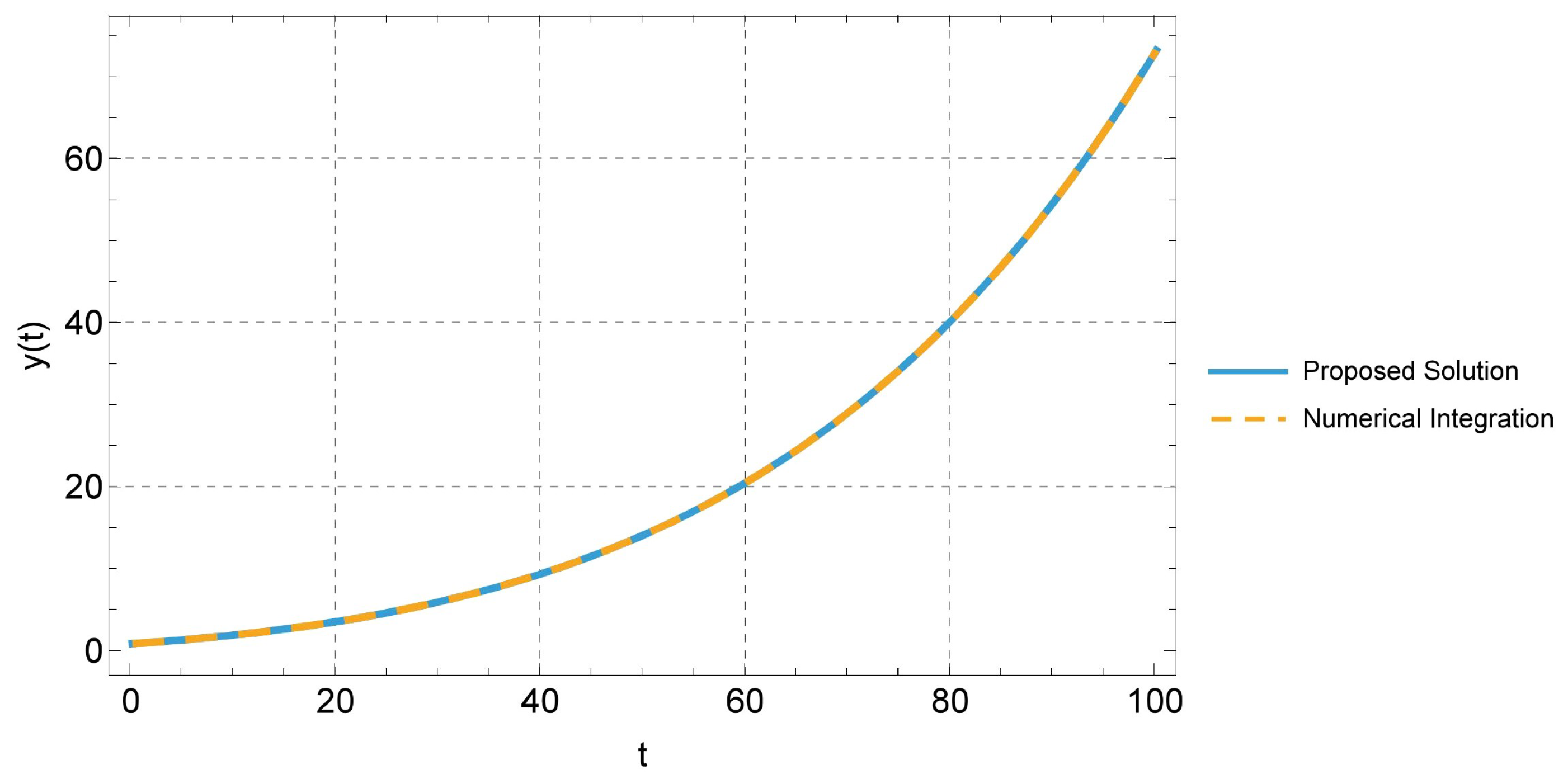
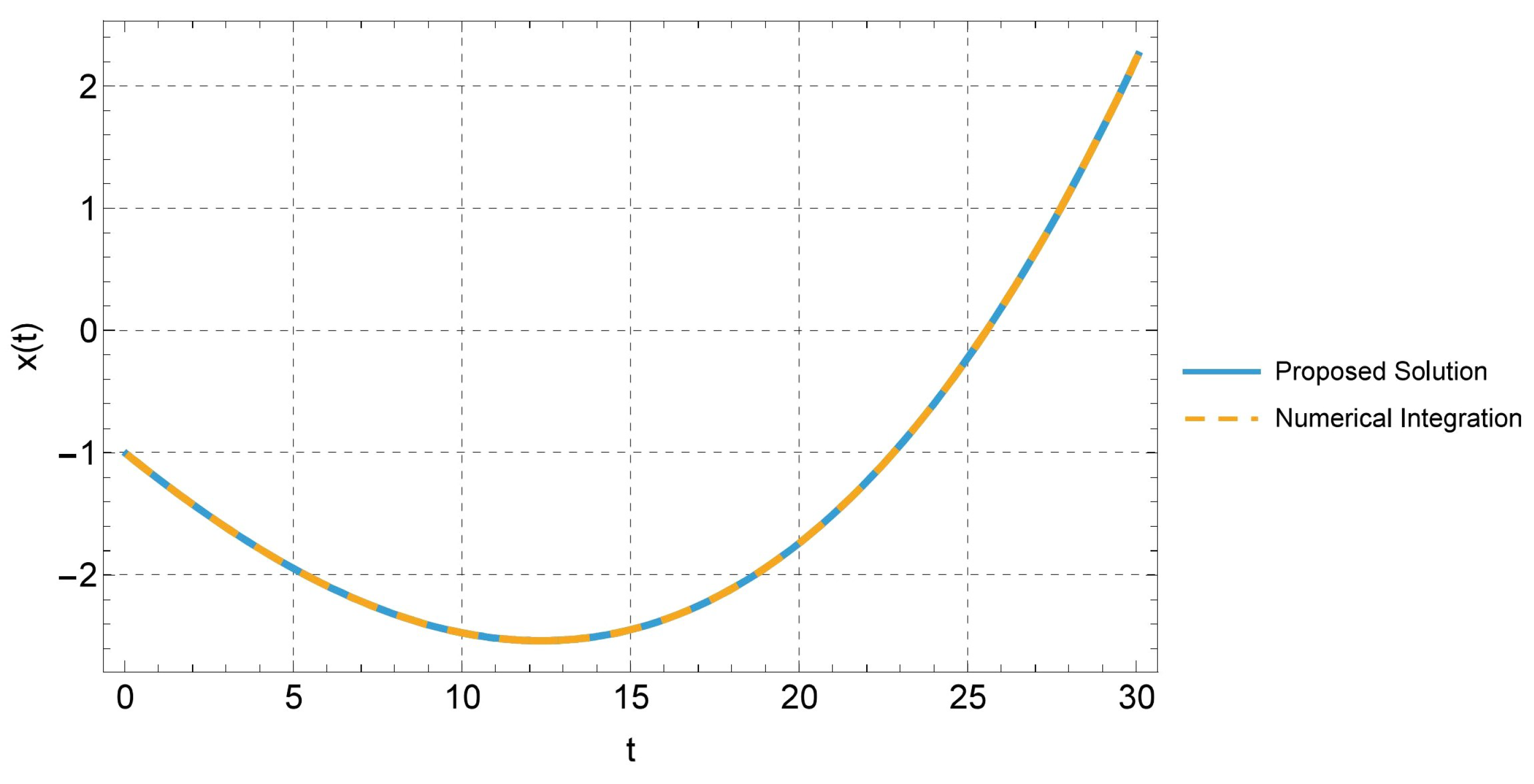
Let r = 2 , m 1 = 3 , m 2 = 2 , A = 1 1 0 1 , x 0 = 1 , and y 0 = 1 . Then c 1 = 6 , c 2 = 5 , c 3 = 1 , and C = 1 / 12 .
Putting Z ( t ) = x ( t ) , y ( t ) T , the components of the solution to the following Cauchy problem are
D 2 L + 5 D L + 6 D x ( t ) , y ( t ) T = A · x ( t ) , y ( t ) T Z ( 0 ) = ( 1 , 1 ) T , Z ( 0 ) = 1 12 A · Z 0 = Z 0 , Z ( 2 ) ( 0 ) = 1 12 A 2 · Z 0 = Z 0 ( 2 )
and are represented in Figure 1 and Figure 2, where a comparison with the proposed method is shown.
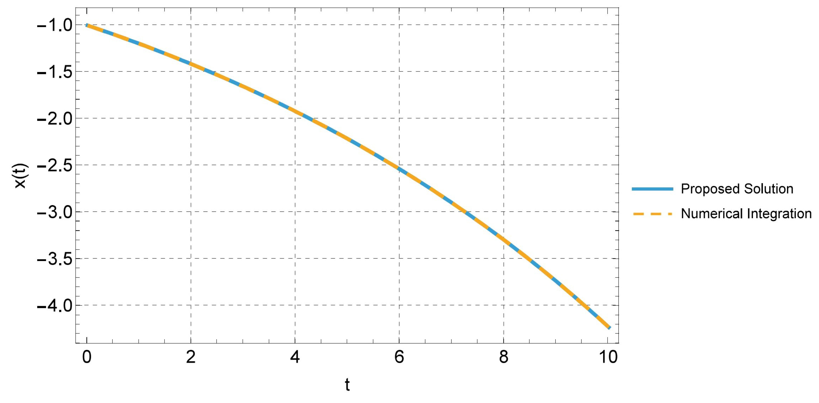
Example 2. 
Let r = 3 , m 1 = 1 , m 2 = 2 , m 3 = 2 ,
A = 1 2 3 2 1 2 3 2 1 ,
x 0 = 1 , y 0 = 0 , and z 0 = 1 . Then c 1 = 4 , c 2 = 8 , c 3 = 5 , c 4 = 1 , and C = 1 / 18 .
Putting Z ( t ) = x ( t ) , y ( t ) , z ( t ) T , the components of the solution to the following Cauchy problem are
D 3 L + 5 D 2 L + 8 D L + 4 D x ( t ) , y ( t ) T = A · x ( t ) , y ( t ) T Z ( 0 ) = ( 1 , 1 ) T , Z ( 0 ) = 1 18 A · Z 0 = Z 0 , Z ( 2 ) ( 0 ) = 1 18 A 2 · Z 0 = Z 0 ( 2 ) , Z ( 3 ) ( 0 ) = 1 18 A 3 · Z 0 = Z 0 ( 3 )
and are represented in Figure 3, Figure 4 and Figure 5, where a comparison with the proposed method is shown.

4.2. Multi-Parametric Population Dynamics Models

Generalizing the results in [30], we consider a multi-parametric extension of the classical Malthus and Verhulst models. Further extensions to the minimum-threshold and Lotka–Volterra models will be considered elsewhere.

4.3. The Multi-Parametric Malthus Case

For example, the multi-parametric Malthus model can be written as follows (see, for details, [31]):
D r L + ( m 1 + m 2 + + m r ) D ( r 1 ) L + + m 1 m 2 m r D P ( t ) = R P ( t ) ,
where R is a positive integer. Upon applying the following initial conditions:
P ( 0 ) = P 0 , P ( 0 ) = C R P 0 = P 0 , P ( r ) ( 0 ) = C R r P 0 = P 0 ( r ) ,
with
C = 1 c 0 + c 1 + + c r ,
the solution is given by
P ( t ) = i = 1 r m i ! e m 1 , m 2 , , m r ( R t ) P 0 .
Example 3. 
Let r = 3 , m 1 = 1 , m 2 = 2 , m 3 = 3 , P 0 = x 0 = 1 , R = 3 . Then c 1 = 6 , c 2 = 11 , c 3 = 6 , c 4 = 1 , C = 1 / 34 .
The solution to the following Mathus problem
D 3 L + 6 D 2 L + 11 D L + 6 D P ( t ) = 3 P ( t ) P ( 0 ) = 1 , P ( 0 ) = 1 8 , P ( 0 ) = 9 34 , P ( 3 ) ( 0 ) = 27 34 ,
according to Equation (17), is given by
P ( t ) = 12 e 1 , 2 , 3 ( 3 t ) = 12 k = 0 ( 3 t ) k k ! ( k + 1 ) ! ( k + 2 ) ! ( k + 3 ) ! .
The relevant graph is represented in Figure 6, where a comparison with the proposed solution is shown.

4.4. The Multi-Parametric Verhulst Case

We consider the following multi-parametric Verhulst model:
D r L + ( m 1 + m 2 + + m r ) D ( r 1 ) L + + m 1 m 2 m r D P ( t ) = R P ( t ) 1 1 K P ( t ) ,
where R is a positive constant, which is called the intrinsic growth rate, and K denotes the environmental capacity.
Upon applying the following initial conditions:
P ( 0 ) = P 0 , P ( 0 ) = C R P 0 1 1 K P 0 = P 0 , P ( r ) ( 0 ) = C R r P 0 1 1 K P 0 = P 0 ( r ) ,
with
C = 1 c 0 + c 1 + + c r ,
the solution is given by
P ( t ) = k = 0 a k t k k ! i = 1 r ( k + m i ) ! ,
where the coefficients a k satisfy the following recursion formula:
a 0 = i = 1 r m i ! P 0 ,
and
a k + 1 = R a k 1 K n = 0 k k ! i = 1 r ( k + m i ) ! a n a k n n ! i = 1 r ( n + m i ) ! ( k n ) ! i = 1 r ( k n + m i ) ! .
Example 4. 
Let r = 3 , m 1 = 1 , m 2 = 2 , m 3 = 3 , P 0 = x 0 = 1 , R = 3 , and K = 2 . Then c 1 = 6 , c 2 = 11 , c 3 = 6 , c 4 = 1 , and C = 1 / 34 .
The solution to the following Mathus problem
D 3 L + 6 D 2 L + 11 D L + 6 D P ( t ) = 3 P ( t ) 1 1 2 P ( t ) P ( 0 ) = 1 , P ( 0 ) = 1 8 1 + 1 2 = 3 16 , P ( 0 ) = 9 34 1 + 1 2 = 27 8 , P ( 3 ) ( 0 ) = 27 34 1 + 1 2 = 81 68 ,
according to Equation (21), is given by
P ( t ) = k = 0 a k t k k ! ( k + 1 ) ! ( k + 2 ) ! ( k + 3 ) ! ,
where the coefficients a k satisfy the following recursion formula:
a 0 = 12 ,
and
a k + 1 = R a k 1 2 n = 0 k k ! ( k + 1 ) ! ( k + 2 ) ! ( k + 3 ) ! a n a k n n ! ( n + 1 ) ! ( n + 2 ) ! ( n + 3 ) ! ( k n ) ! ( k n + 1 ) ! ( k n + 2 ) ! ( k n + 3 ) ! .
The relevant graph is represented in Figure 7, where a comparison with the proposed solution is shown below.

5. Further Applications

Extending the results that are shown in [27], one can consider the multi-parametric Bernoulli and Euler numbers and the related polynomials, starting from the following definitions:
Multi-parametric Bernoulli numbers:
t e m 1 , m 2 , , m r ( t ) 1 = n = 0 B ( m 1 , m 2 , , m r | n ) t n n ! .
Multi-parametric Bernoulli polynomials:
t e m 1 , m 2 , , m r ( x t ) e m 1 , m 2 , , m r ( t ) 1 = n = 0 B ( m 1 , m 2 , , m r | n ) ( x ) t n n ! .
Multi-parametric Euler numbers:
2 e m 1 , m 2 , , m r ( t ) e m 1 , m 2 , , m r ( 2 t ) + 1 = n = 0 E ( m 1 , m 2 , , m r | n ) t n n ! .
Multi-parametric Euler polynomials:
2 e m 1 , m 2 , , m r ( x t ) e m 1 , m 2 , , m r ( t ) + 1 = n = 0 E ( m 1 , m 2 , , m r | n ) ( x ) t n n ! .

The Case of the Fractional Derivatives

Extensions of the above results deal with the use of fractional derivatives by introducing the multi-parametric fractional operators defined as follows:
D t α [ t α D t α + m 1 ] [ t α D t α + m 2 ] [ t α D t α + m r ] = D r L α + ( m 1 + m 2 + + m r ) D ( r 1 ) L α + + m 1 m 2 m r D α D α : = D t α .
This is not a trivial topic, and it is not sufficient to change the factorials into their expressions using the familiar (Euler’s) Gamma function Γ ( · ) , but it needs a deeper analysis. In addition to those that are extensively and comprehensively analyzed in the above-cited survey-cum-expository paper [17], the interested readers may find useful information in the vast literature on the various existing operators of fractional integrals and fractional derivatives (see, for example, [32,33,34,35,36,37]).
In forthcoming articles, some of the above-mentioned topics will be examined in detail. We choose to cite a number of potentially useful works on the hyper-Bessel type functions and the related operational calculus [38,39,40,41,42] as well as on mathematical biology (see, for example, [43,44,45]).

6. Conclusions

Here, in our present investigation, we have applied and exploited some multi-parametric forms of functions that behave as exponentials with respect to suitable Laguerre-type differential operators in order to introduce extensions of some classical mathematical models. In particular, we have introduced multi-parametric versions of linear dynamical systems and population dynamics models.
Multi-parametric extensions of classical entities from number theory, such as the Bernoulli and Euler numbers and the related generalized polynomial systems, have also been suggested herein.
Numerical verifications, which are constructed using the computer graphics program Mathematica© (Version 14.3), have been shown throughout our investigation.

Author Contributions

Conceptualization, H.M.S. and P.E.R.; Methodology, D.C. and P.E.R.; Validation, H.M.S., D.C., and P.E.R.; Software, D.C.; Validation, H.M.S., D.C., and P.E.R.; Formal Analysis, H.M.S., D.C., and P.E.R.; Investigation, D.C. and P.E.R.; Resources, H.M.S., D.C., and P.E.R.; Writing—Original Draft Preparation, D.C. and P.E.R.; Writing—Review and Editing, H.M.S. and P.E.R.; Supervision, H.M.S. and P.E.R. All authors have read and agreed to the published version of the manuscript.

Funding

This research received no external funding.

Data Availability Statement

The data are available upon request to the second author.

Conflicts of Interest

The authors declare that they have no conflicts of interest.

Appendix A

Axioms 14 00705 i001
Axioms 14 00705 i002

References

  1. Kilbas, A.A.; Koroleva, A.A.; Rogosin, S.V. Multi-parametric Mittag-Leffler functions and their extension. Fract. Calc. Appl. Anal. 2013, 16, 378–404. [Google Scholar] [CrossRef]
  2. Kiryakova, V. Multiple Dzrbashjan-Gelfond-Leontiev fractional differintegrals. In Proceedings of the Recent Advances in Applied Mathematics (Workshop RAAM’96), Kuwait City, Kuwait, 4–7 May 1996; pp. 281–294. [Google Scholar]
  3. Kiryakova, V. Multiple (multi-index) Mittag-Leffler functions and relations to generalized fractional calculus. J. Comput. Appl. Math. 2000, 118, 241–259. [Google Scholar] [CrossRef]
  4. Kiryakova, V. The multi-index Mittag-Leffler functions as an important class of special functions of fractional calculus. Comput. Math. Appl. 2010, 59, 1885–1895. [Google Scholar] [CrossRef]
  5. Paneva-Konovska, J. A survey on Bessel type functions as multi-index Mittag-Leffler functions: Differential and integral relations. Internat. J. Appl. Math. 2019, 32, 357–380. [Google Scholar] [CrossRef]
  6. Paneva-Konovska, J. Hyper-Bessel functions as multi-index Mittag-Leffler functions: Integrals and derivatives of arbitrary orders. In Proceedings of the 45th International Conference on Application of Mathematics in Engineering and Economics (AMEE’19), Sozopol, Bulgaria, 7–13 June 2019; Volume 2172, p. 050005. [Google Scholar] [CrossRef]
  7. Aljohani, A.F.; Ebaid, A.; Algehyne, E.A.; Mahrous, Y.M.; Cattani, C.; Al-Jeaid, H.K. The Mittag-Leffler function for re-evaluating the chlorine transport model: Comparative analysis. Fractal Fract. 2022, 6, 125. [Google Scholar] [CrossRef]
  8. Ebaid, A.; Cattani, C.; Al Juhani, A.S.; El-Zahar, E.R. A novel exact solution for the fractional Ambartsumian equation. Adv. Differ. Equ. 2021, 2021, 88. [Google Scholar] [CrossRef]
  9. Prabhakar, T.R. A singular integral equation with a generalized Mittag-Leffler function in the kernel. Yokohama Math. J. 1971, 19, 7–15. [Google Scholar]
  10. Caratelli, D.; Ricci, P.E. Laguerre-type fractional parametric population dynamics models. Appl. Nonlinear Anal. 2025, 1, 1–13. [Google Scholar]
  11. Mishra, A. Special Integrals; Series on University Texts in the Mathematical Sciences; Springer Nature: Singapore; Private Limited: Singapore, 2025. [Google Scholar] [CrossRef]
  12. Srivastava, H.M. Some families of Mittag-Leffler type functions and associated operators of fractional calculus. TWMS J. Pure Appl. Math. 2016, 7, 123–145. [Google Scholar]
  13. Fox, C. The asymptotic expansion of generalized hypergeometric functions. Proc. London Math. Soc. 1928, 27, 389–400. [Google Scholar] [CrossRef]
  14. Wright, E.M. The asymptotic expansion of the generalized hypergeometric function. J. London Math. Soc. 1935, 10, 284–293. [Google Scholar] [CrossRef]
  15. Wright, E.M. The asymptotic expansion of the generalized hypergeometric function. Proc. London Math. Soc. 1940, 46, 389–408. [Google Scholar] [CrossRef]
  16. Erdélyi, A.; Magnus, W.; Oberhettinger, F.; Tricomi, F.G. Higher Transcendental Functions; McGraw-Hill Book Company: New York, NY, USA; Toronto, ON, Canada; London, UK, 1953; Volume I. [Google Scholar]
  17. Srivastava, H.M. A survey of some recent developments on higher transcendental functions of analytic number theory and applied mathematics. Symmetry 2021, 13, 2294. [Google Scholar] [CrossRef]
  18. Barnes, E.W. The asymptotic expansion of integral functions defined by Taylor’s series. Philos. Trans. Roy. Soc. London Ser. A Math. Phys. Sci. 1906, 206, 249–297. [Google Scholar]
  19. Wright, E.M. The asymptotic expansion of integral functions defined by Taylor series. I. Philos. Trans. Roy. Soc. London Ser. A Math. Phys. Sci. 1940, 238, 423–451. [Google Scholar]
  20. Wright, E.M. The asymptotic expansion of integral functions defined by Taylor series. II. Philos. Trans. Roy. Soc. London Ser. A Math. Phys. Sci. 1941, 239, 217–232. [Google Scholar]
  21. Wright, E.M. The asymptotic expansion of integral functions and of the coefficients in their Taylor series. Trans. Amer. Math. Soc. 1948, 64, 409–438. [Google Scholar] [CrossRef]
  22. Mittag-Leffler, G.M. Sur la nouvelle fonction Eα(x). C. R. Acad. Sci. Paris 1903, 137, 554–558. [Google Scholar]
  23. Hilfer, R.; Seybold, H.J. Computation of the generalized Mittag-Leffler function and its inverse in the complex plane. Integral Transforms Spec. Funct. 2006, 17, 637–652. [Google Scholar] [CrossRef]
  24. Haubold, H.J.; Mathai, A.M.; Saxena, R.K. Mittag-Leffler functions and their applications. J. Appl. Math. 2011, 2011, 298628. [Google Scholar] [CrossRef]
  25. Mainardi, F. Why the Mittag-Leffler function can be considered the queen function of the fractional calculus? Entropy 2020, 22, 1359. [Google Scholar] [CrossRef] [PubMed]
  26. Caratelli, D.; Ricci, P.E. A note on fractional-type models of population dynamics. Math. Model. Anal. Vilnius Tech. 2023, 29, 480–492. [Google Scholar] [CrossRef]
  27. Caratelli, D.; Natalini, P.; Ricci, P.E. Fractional Bernoulli and Euler numbers and related fractional polynomials: A symmetry in number theory. Symmetry 2023, 15, 1900. [Google Scholar] [CrossRef]
  28. Ricci, P.E.; Srivastava, R.; Caratelli, D. Laguerre-type Bernoulli and Euler numbers and related fractional polynomials. Mathematics 2024, 12, 381. [Google Scholar] [CrossRef]
  29. Natalini, P.; Ricci, P.E. Laguerre-type linear dynamical systems. Ilirias J. Math. 2015, 4, 24–40. [Google Scholar]
  30. Caratelli, D.; Natalini, P.; Ricci, P.E. Laguerre-type parametric population dynamics models. J. Nonlinear Sci. Appl. 2025, 18, 239–249. [Google Scholar] [CrossRef]
  31. Almeida, R.; Bastos, N.R.O.; Monteiro, M.T.T. A fractional Malthusian growth model with variable order using an optimization approach. Statist. Optim. Inform. Comput. 2018, 6, 4–11. [Google Scholar] [CrossRef]
  32. Samko, S.G.; Kilbas, A.A.; Marichev, O.I. Fractional Integrals and Derivatives: Theory and Applications; Gordon and Breach Science Publishers: Yverdon, Switzerland, 1993. [Google Scholar]
  33. Kiryakova, V. Generalized Fractional Calculus and Applications; Pitman Research Notes in Mathematics Series, No. 301; Longman: Harlow, UK, 1994. [Google Scholar]
  34. Podlubny, I. Fractional Differential Equations: An Introduction to Fractional Derivatives, Fractional Differential Equations, to Methods of Their Solution and Some of Their Applications, Mathematics in Science and Engineering; Academic Press: New York, NY, USA; London, UK; Sydney, NSW, Australia; Tokyo, Japan; Toronto, ON, Canada, 1999; Volume 198. [Google Scholar]
  35. Hilfer, R. (Ed.) Applications of Fractional Calculus in Physics; World Scientific Publishing Company: Singapore; Newark, NJ, USA; London, UK; Hong Kong, China, 2000. [Google Scholar]
  36. Kilbas, A.A.; Srivastava, H.M.; Trujillo, J.J. Theory and Applications of Fractional Differential Equations; North-Holland Mathematical Studies; Elsevier (North-Holland) Science Publishers: Amsterdam, The Netherlands; London, UK; New York, NY, USA, 2006; Volume 204. [Google Scholar]
  37. Anastassiou, G.A. Generalized Fractional Calculus: New Advancements and Applications; Studies in Systems, Decision and Control; Springer: Cham, Switzerland, 2021; Volume 305. [Google Scholar]
  38. Dattoli, G. Hermite-Bessel and Laguerre-Bessel functions: A by-product ot the monomiality principle. In Advanced Special Functions and Applications, Proceedings of the Melfi School on Advanced Topics in Mathematics and Physics, Melfi, Italy, 9–12 May 1999; Cocolicchio, D., Dattoli, G., Srivastava, H.M., Eds.; Aracne Editrice: Rome, Italy, 2000; pp. 147–164. [Google Scholar]
  39. Delerue, P. Sur le calcul symbolique à n variables et fonctions hyper-besséliennes (II). Ann. Soc. Sci. Bruxelles 1953, 3, 229–274. [Google Scholar]
  40. Dimovski, I. Operational calculus for a class of differential operators. C. R. Acad. Bulgare Sci. 1966, 19, 1111–1114. [Google Scholar]
  41. Ditkin, A.P.; Prudnikov, V.A. Transforms and Operational Calculus; Pergamon Press: Oxford, UK, 1965. [Google Scholar]
  42. Gause, G.F. Vérifications Expérimentales de la Théorie Mathématique de la lutte pour la vie. In No. 277 of the Series on Actualités Scientifiques et Industrielles (Volume 9 of the Exposés de Biométrie et de Statistique Biologique); Hermann and Company: Paris, France, 1935. [Google Scholar]
  43. Alee, W.C. Animal Aggregations; University of Chicago Press: Chicago, IL, USA, 1931. [Google Scholar]
  44. Murray, J. Mathematical Biology; Springer: Berlin/Heidelberg, Germany; New York, NY, USA, 1989. [Google Scholar]
  45. Thieme, H.R. Mathematics in Population Biology; Princeton University Press: Princeton, NJ, USA, 2003. [Google Scholar]
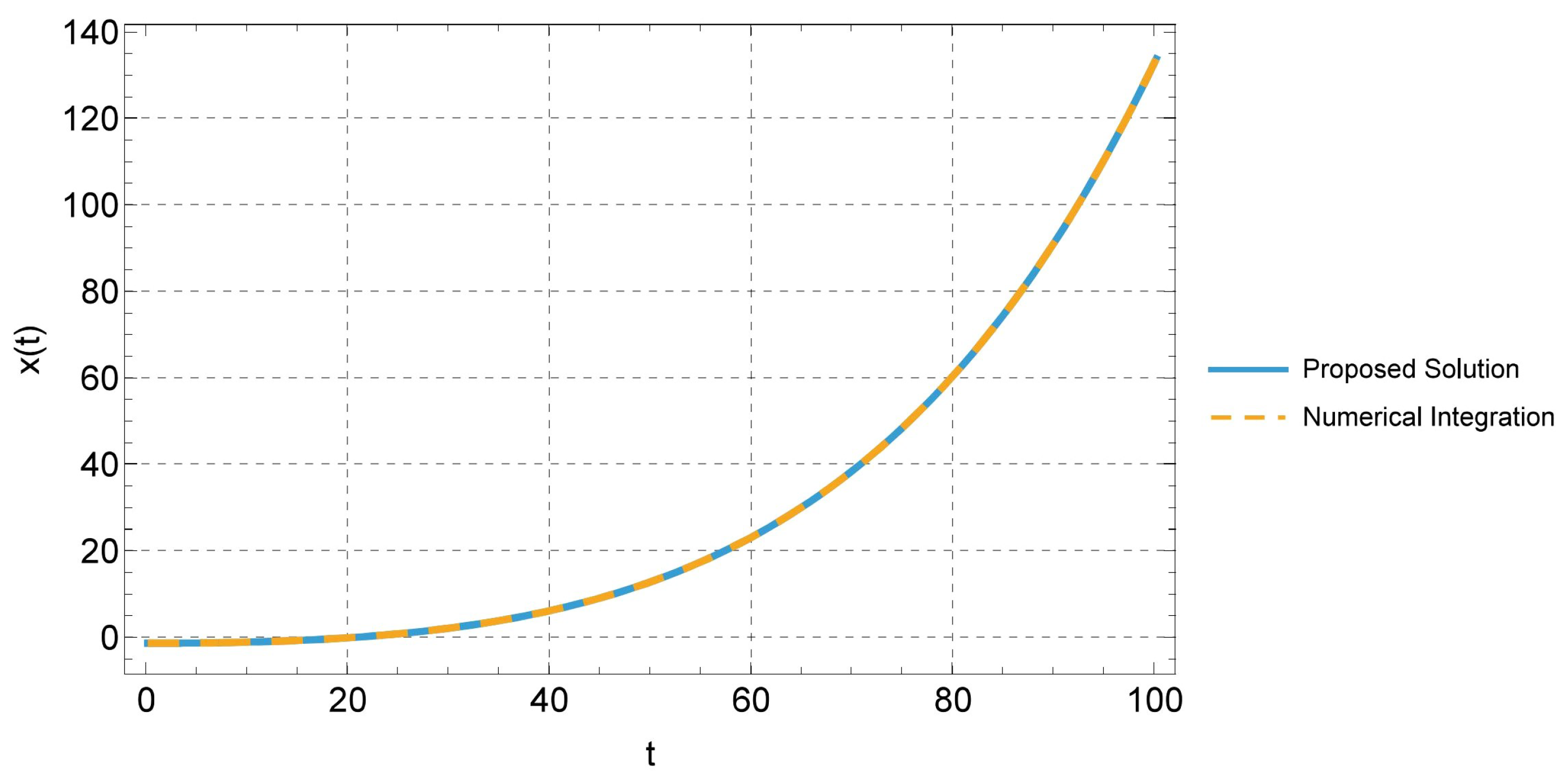
Figure 1. The component x ( t ) of the solution to the Cauchy problem in Example 1.
Axioms 14 00705 g001
Figure 2. The component y ( t ) of the solution to the Cauchy problem in Example 1.
Axioms 14 00705 g002
Figure 3. The component x ( t ) of the solution to the Cauchy problem in Example 2.
Axioms 14 00705 g003
Figure 4. The component y ( t ) of the solution to the Cauchy problem in Example 2.
Axioms 14 00705 g004
Figure 5. The component z ( t ) of the solution to the Cauchy problem in Example 2.
Axioms 14 00705 g005
Figure 6. The solution to the Malthus problem in Example 3, where x ( t ) = P ( t ) .
Axioms 14 00705 g006
Figure 7. The solution to the Verhulst problem in Example 4, where x ( t ) = P ( t ) .
Axioms 14 00705 g007
Disclaimer/Publisher’s Note: The statements, opinions and data contained in all publications are solely those of the individual author(s) and contributor(s) and not of MDPI and/or the editor(s). MDPI and/or the editor(s) disclaim responsibility for any injury to people or property resulting from any ideas, methods, instructions or products referred to in the content.