5.1. Performance of and Indices
The following simulation experiments were conducted on the new indices
and
, and the results were compared with the true process capability values
and
in order to determine whether the new indices based on truncated sample theory can evaluate the process capability of the observed samples more accurately. The comparison also includes the
and
indices without taking truncation information into account, in order to more clearly show the efficacy of the suggested approach. Here,
and
are calculated in Formulas (
24) and (
25);
and
are defined in Formulas (
19) and (
21); and the estimating formulas for
and
are presented in Equations (
20) and (
22).
The comparison experiment was conducted from three aspects. First, by controlling the number of samples and the expectation and variance of the sample as a whole, and varying the position of the left-truncated point, we explored the impact of different cutoff point positions on the estimation of and . Second, by controlling the position of the left-truncated point and the expectation and variance of the sample as a whole, and letting the number of samples grow from small to large, we studied the impact of different sample sizes on the accuracy of the estimation results.
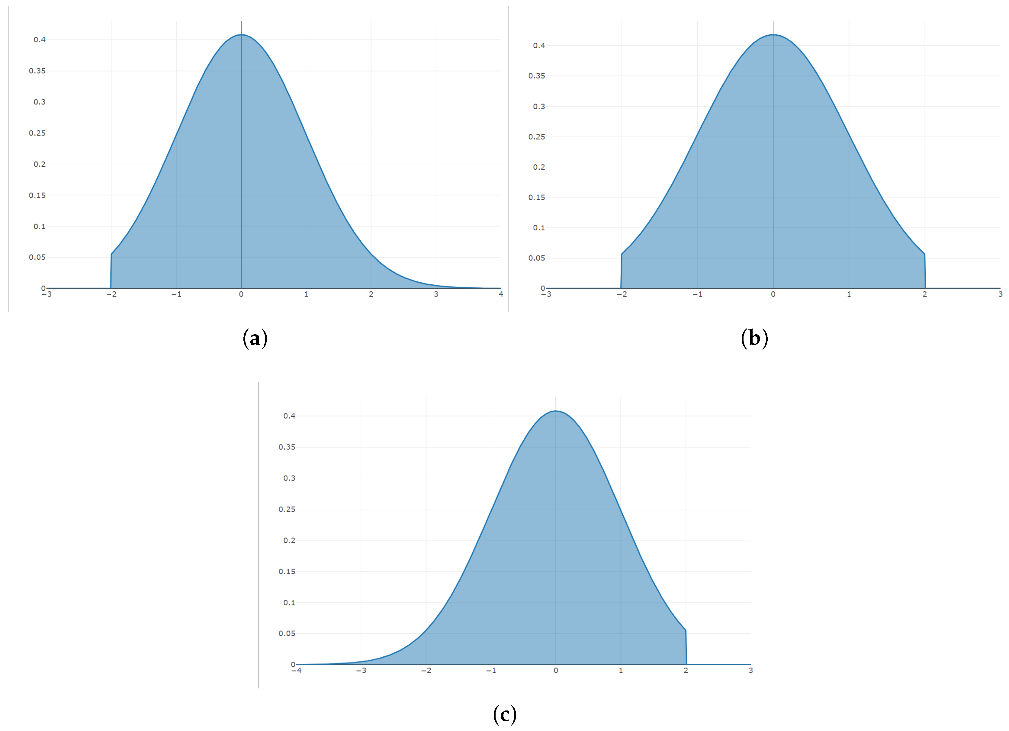
Since any normal distribution can be converted to a normal distribution, without loss of generality, the first two sets of simulation experiments use standard normal distribution observations, i.e., the population
. The upper and lower specification lines are designed as
,
, respectively. Thus, the true process capability value of the sample is as follows:
All experiments were conducted on a PC using R software. All simulations were performed 10,000 times, with the average value being used as the final result in order to make the experimental results representative, given the random nature of sample collection.
Experiment 1. Set the observation sample size as
, and let the value of the truncation point
a change from
to 3 in intervals of 0.1. Then, generate
n random truncated samples using the rnormTrunc() function in the EnvStats package with parameter
a as the truncation point, and estimate the values of
,
,
, and
using Equations (
20), (
22), (
24), and (
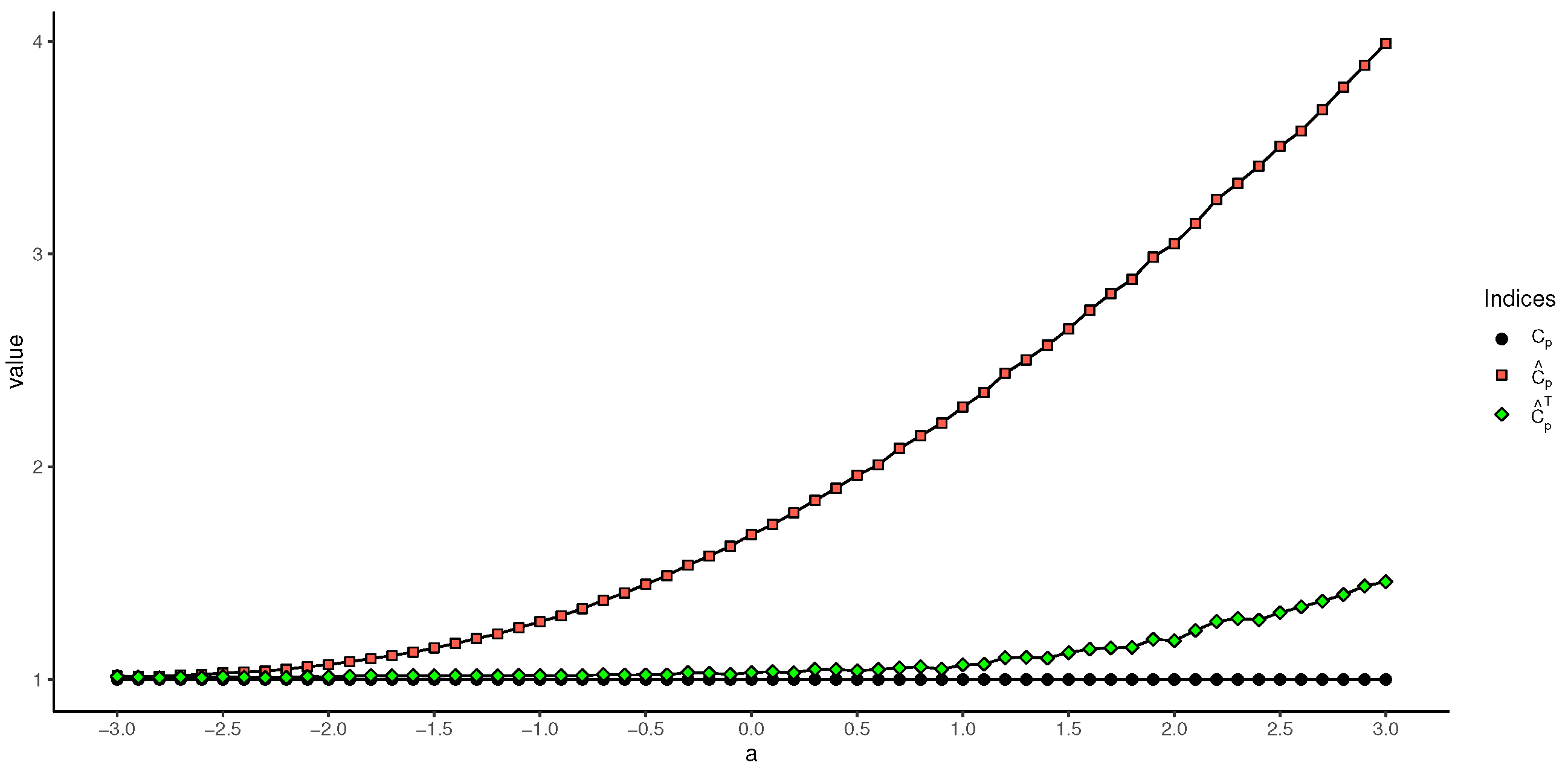
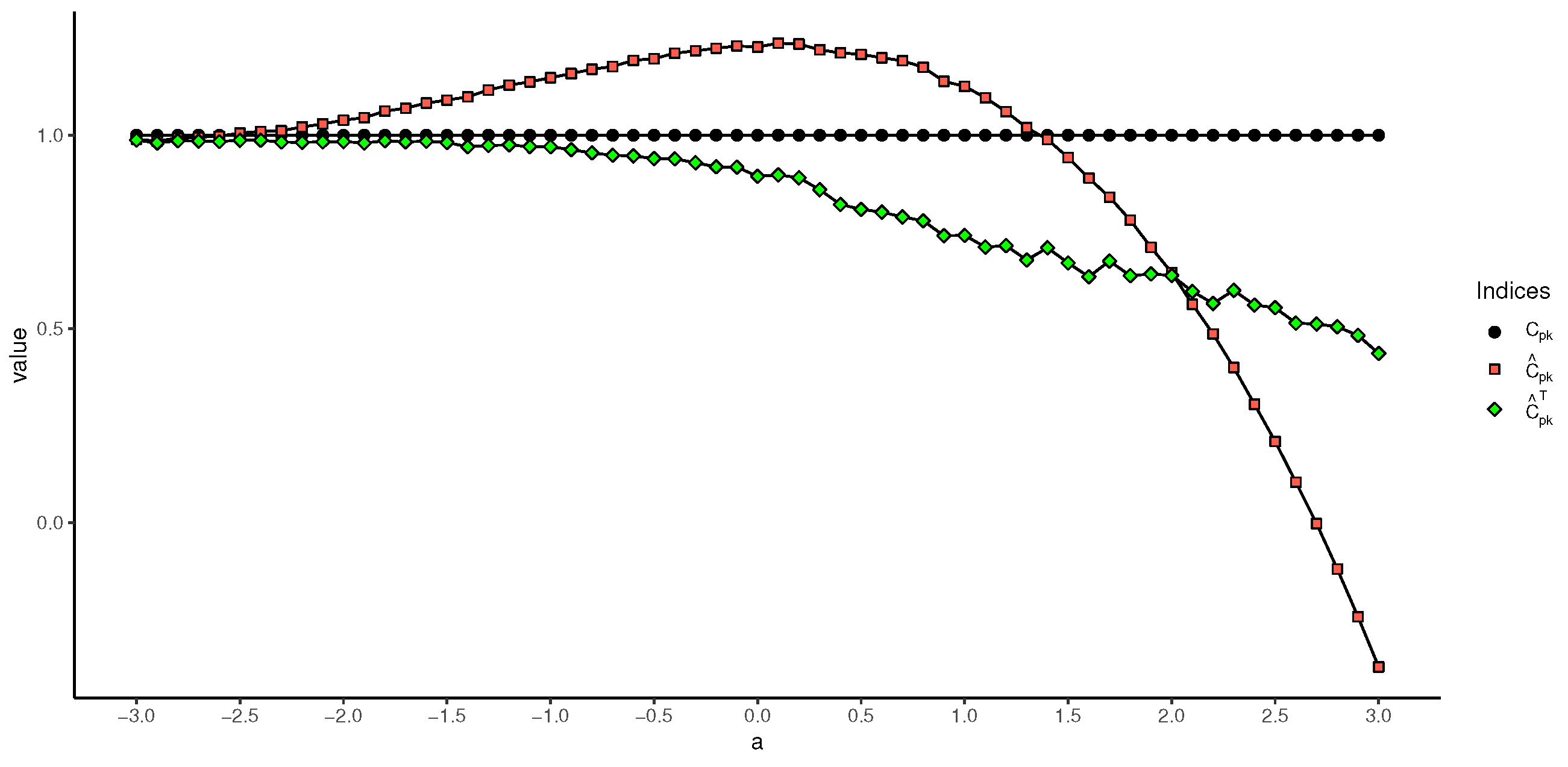
25), respectively. The results are shown in
Figure 3 and
Figure 4.
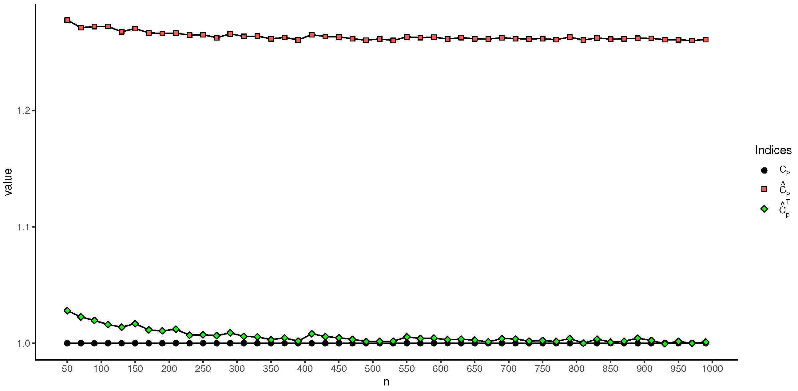
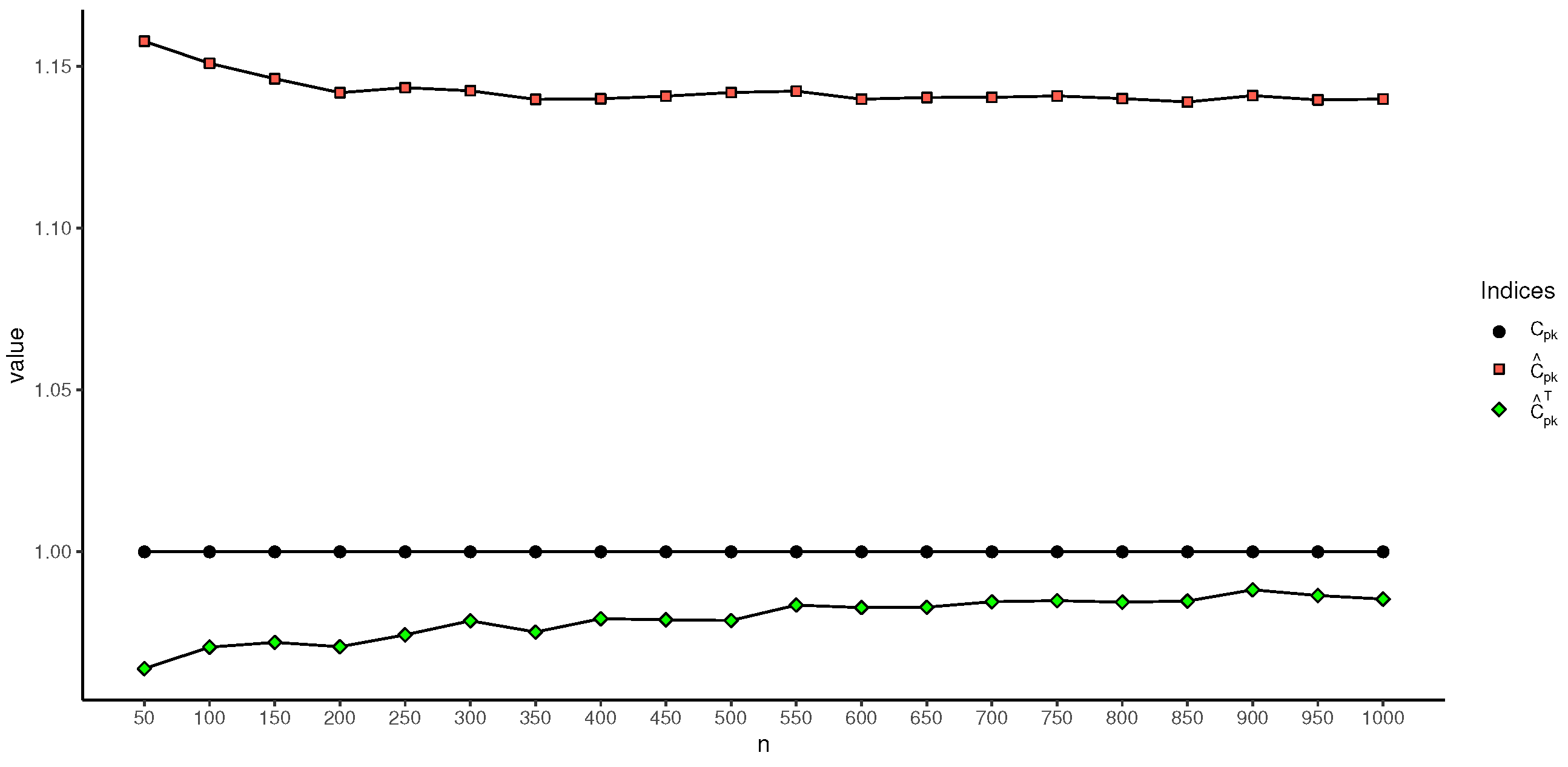
As can be seen in
Figure 3 and
Figure 4, the difference between
and
, as well as the difference between
and
, increases with the growing value of the truncation point, i.e., if the truncation information of the sample is not taken into account when calculating the process capability index for truncated samples, the final estimated result will be higher than the true value. For the newly proposed estimation method, the results of
and
slowly increase and drop, respectively. Nevertheless, both
and
outperform
and
. Moreover, on the left side of the symmetry axis
, the difference between the estimates of
and
and the true values of
and
is very small, which implies that the proposed two process capability indices have a good chance of being applied when the truncation point is on the left side of the symmetry axis.
Experiment 2. Another issue we are concerned about is how the accuracy of the proposed index estimation varies with changes in the sample size. Understanding this issue will assist users in determining the appropriate sample size for practical applications. In this experiment, we compare the results of different estimations with the true values. To assess the sensitivity of the proposed method to sample size, the number of samples was increased progressively from 50 to 1000, and the truncation point was set to −2, −1, 0, 1, and 2, respectively. The simulated results are shown in
Table 3 and
Table 4.
Table 3 and
Table 4 show that, when the cutoff value is controlled, the estimation results for
and
converge to the true value
, whereas
and
also converge to the true value with the increase in the sample size. However, there is always a significant difference between the estimation results
and
, and the true values of
and
. This phenomenon can be further seen in
Figure 5 and
Figure 6. When the truncation value is set to
, as can be seen, the
and
indices, which account for truncation information, outperform
and
in terms of estimating effect. Additionally,
Table 3 and
Table 4 show that when the truncated value increases, the estimation results for the
index deteriorate; when the sample size is greater than 100, the estimation results for the newly proposed
index are much closer to the true value. In addition, it can also be seen from
Table 3 and
Table 4 that, for the estimation of the
index, the results of the
index estimates become worse as the truncation value increases. However, the proposed
index does not differ much from the true values when the sample size is greater than 100. For the performance of the
index estimator, the performance of
still outperforms that of
.
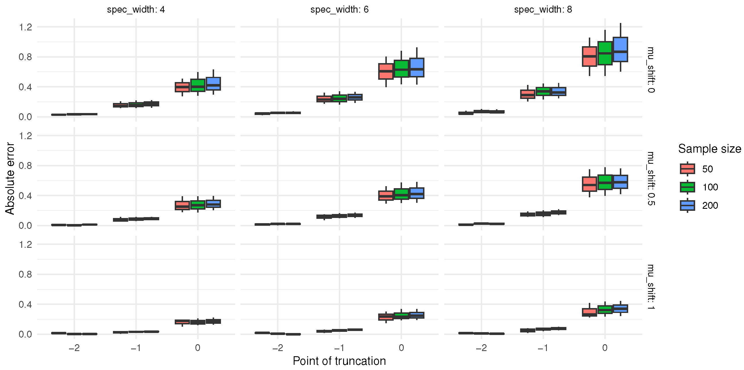
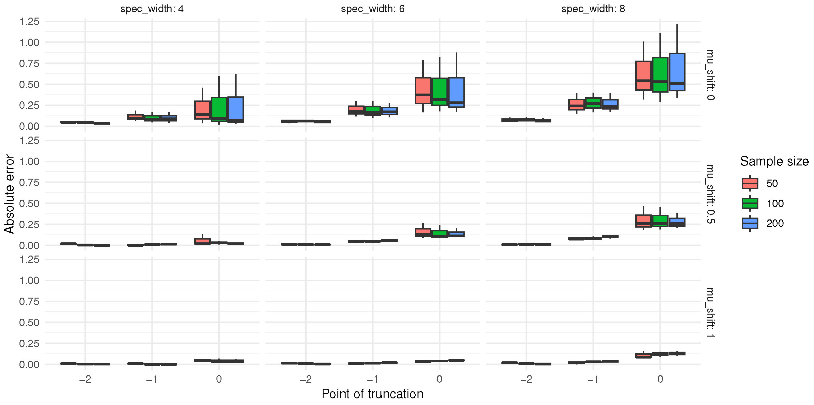
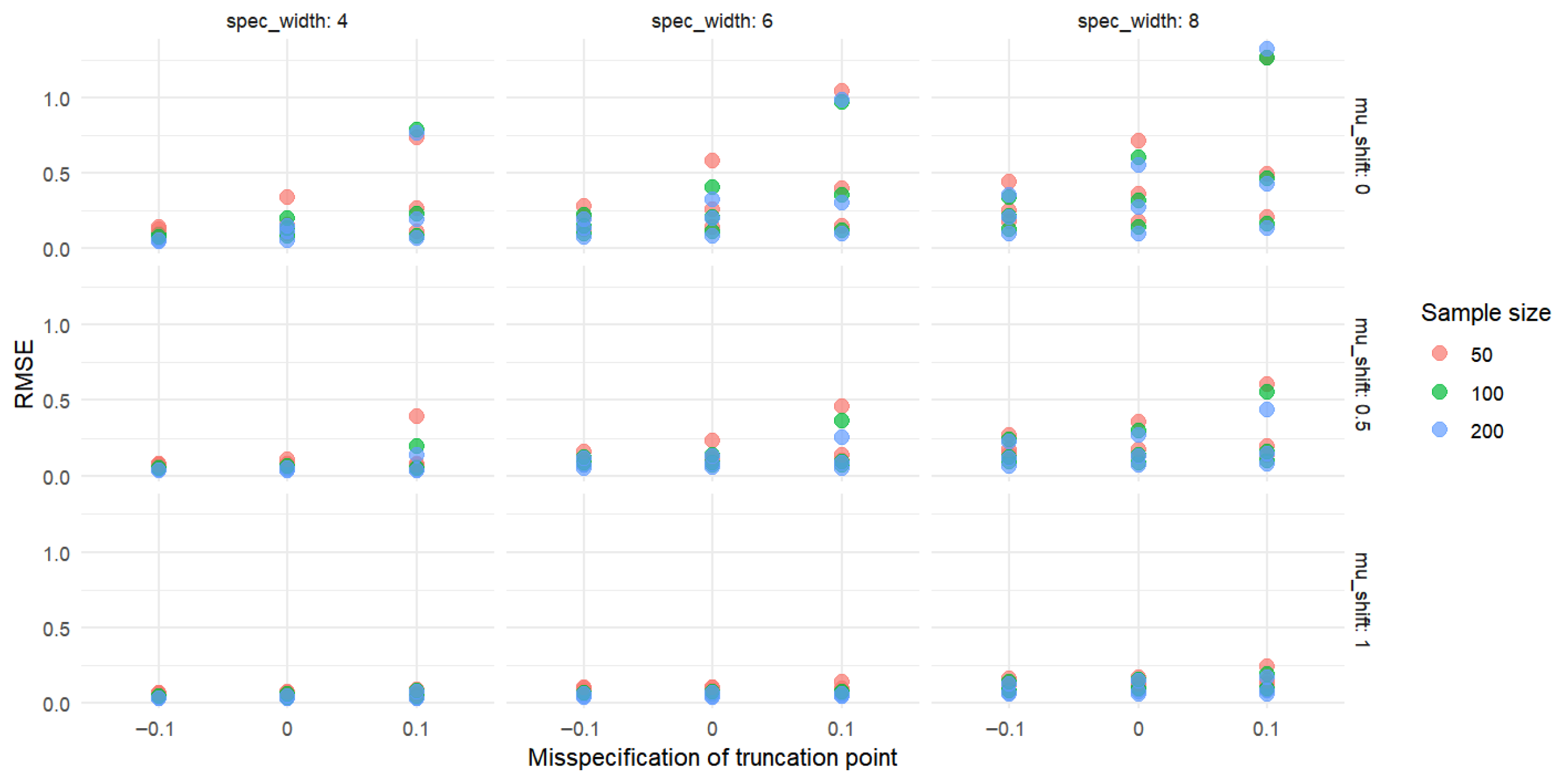
Experiment 3. To further investigate the absolute bias and root mean square error (RMSE) values of
and
under varying sample sizes, censoring rates, and mean shifts, Experiment 3 was designed. The absolute biases of the modified indices are presented in
Figure 7 and
Figure 8, while the RMSE results are shown in
Figure 9 and
Figure 10.
Analysis of the data in
Figure 7 and
Figure 8 reveals certain patterns in the absolute biases of
and
under different sample sizes, censoring levels (indicated by the censoring point), and mean shifts. When the sample size is 50, under various censoring points, the absolute biases of both
and
generally decrease as the mean shift increases. Moreover, a larger censoring point (i.e., a lower degree of censoring) corresponds to greater absolute biases under the same mean shift. Similar trends are observed for a sample size of 100. Compared to the case with a sample size of 50, the absolute biases tend to decrease in some scenarios. When the sample size increases to 200, these patterns become more pronounced, and the absolute biases are further reduced in certain cases compared to those with a sample size of 100.
Overall, as the sample size increases, the absolute biases of and tend to decrease under the same censoring level and mean shift. For a fixed sample size, a lower degree of censoring (i.e., larger censoring point) generally leads to higher absolute bias. In addition, as the mean shift increases, the absolute biases of and mostly exhibit a declining trend. These findings indicate that sample size, censoring level, and mean shift all influence the absolute biases of and . In practical applications, these patterns can be utilized to optimize relevant operations or improve prediction accuracy.
As shown in
Figure 9 and
Figure 10, from the perspective of sample size, when the censoring level and mean shift are fixed, the RMSE values of both
and
generally exhibit a decreasing trend as the sample size increases from 50 to 200. For example, at a censoring point of −2 and a mean shift of 0, the RMSE of cpt decreases from 0.359639 (sample size 50) to 0.315073 (sample size 100), and further to 0.283292 (sample size 200); similarly, the RMSE of cpkt decreases from 0.375543 (sample size 50) to 0.329441 (sample size 100), and then to 0.287575 (sample size 200). These results indicate that larger sample sizes may contribute to reducing the RMSE values of
and
.
Regarding the censoring level, under the same sample size and mean shift, a larger censoring point (i.e., lower degree of censoring) tends to correspond to higher RMSE values for both and . For instance, at a sample size of 100 and a mean shift of 0, as the censoring point changes from −2 to 0, the RMSE of cpt increases from 0.315073 to 0.808805, and that of cpkt rises from 0.329441 to 0.688743.
In terms of the effect of mean shift, when the sample size and censoring level are fixed, the RMSE values of and mostly show a decreasing trend as the mean shift increases. Taking a sample size of 50 and a censoring point of −1 as an example, the RMSE of cpt decreases from 0.536742 (mean shift 0) to 0.363781 (mean shift 1), while the RMSE of cpkt drops from 0.520519 (mean shift 0) to 0.303010 (mean shift 1).
5.2. Bootstrap Confidence Interval for and Indices
One of the hotspots that researchers and quality managers are concerned about is the impact of shortened samples on process capability. According to
Section 4.1, the truncation position can be found in a variety of places, and the sample size or truncation value will affect how accurately the process capability indices are estimated. The following simulation studies examine the interval estimation of the
and
indices under different parameter situations; the interval estimation of the
and
indices with different sample sizes and different truncation point locations is simulated below. This is done in order to further analyze the effect of samples containing truncation information on the interval estimation of the process capability indices.
The sample size
n for the simulations that follow was changed from 50, 100, and 200 to 500, and the truncation values
were selected with
and
. Using R software, random samples were created, the procedure was repeated 10,000 times, and the random seed was set to 123. The 95% SB confidence intervals of the
and
indices calculated by the traditional and proposed methods are shown in
Table 5 and
Table 6.
In
Table 5 and
Table 6,
and
denote the lower and upper confidence intervals of the estimated parameter
. As can be seen from
Table 5, the upper and lower confidence intervals of both
and
are larger than the true value
, which indicates that when the truncation information exists, both
and
are overestimated. But this overestimation is inversely proportional to the change in sample size. Moreover, the
index is overestimated to a much smaller extent than the
index, and this tendency is reflected more clearly with the rightward shift of the truncation point. For example, when
and
, the confidence interval of
is
, and the confidence interval of
is
. At this point, the length of the confidence interval of
is 0.012, which is smaller than the length of the confidence interval of
, 0.014, and it is closer to the true
value. However, when the sample size increases, the advantage of the
confidence interval estimation results is quickly lost. For example, when
,
,
’s confidence interval
is obviously better than
’s confidence interval
, even though the lengths of their confidence intervals are the same.
If the sample is controlled so that the truncation position is gradually moved from −3 to 3, the confidence interval estimation advantage of the index becomes more evident than that of the index. For example, under the condition of a sample size of 50, when , the confidence interval of the index, , is far better than that of the index .
The same experiment becomes a little more complicated for the
index. First of all, in the estimation of the
index,
will always be underestimated, while
is overestimated when the truncation point is located on the left side of the symmetry axis. When the truncation point is moved to the right side of the symmetry axis, the estimation of the
quickly becomes underestimated. This phenomenon can be seen in
Figure 5 and
Table 6.
Overall, the index estimate without considering truncation information may outperform the index only when the truncation point is located within . In the rest of the cases, the index, which considers sample truncation information, outperforms the index in confidence interval estimation.
Combining the results from
Table 5 and
Table 6, it is clear that the proposed new indices
and
outperform conventional estimation techniques in the majority of cases without taking into account sample truncation information in the confidence interval estimation. This shows that in the application of actual industrial production, we cannot ignore the existence of truncation information, especially for samples sent for testing in order to pass inspection. It is particularly noteworthy that both of the newly proposed indices show surprising accuracy when the truncation position of the sample is on the left side of the symmetry axis, for both point and interval estimation.
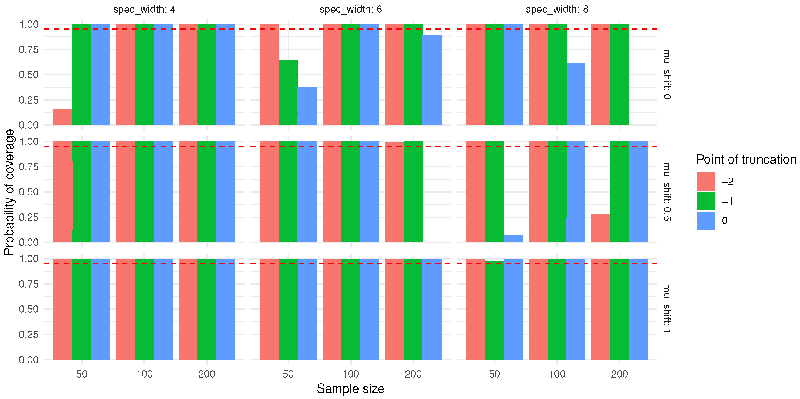
Building on the experiments above, we now discuss the bootstrap interval coverage of the true value under varying sample sizes, censoring rates, and mean shifts. The results are shown in
Figure 5 and
Figure 6As shown in
Figure 11 and
Figure 12, from the perspective of sample size, when the censoring level and mean shift are held constant, the bootstrap interval coverage of the true value of both
and
generally exhibit a decreasing trend as the sample size increases from 50 to 200. For instance, at a censoring point of −2 and a mean shift of 0, the bootstrap interval coverage of the true value of
decreases from 0.36 (sample size 50) to 0.32 (sample size 100), and further to 0.28 (sample size 200). Similarly, the bootstrap interval coverage of the true value of
declines from 0.38 (sample size 50) to 0.33 (sample size 100), and then to 0.29 (sample size 200). These results suggest that larger sample sizes may help reduce the RMSE values of
and
.
With respect to the censoring level, under the same sample size and mean shift, a larger censoring point (i.e., lower degree of censoring) tends to correspond to higher RMSE values for both and . For example, at a sample size of 100 and a mean shift of 0, as the censoring point increases from −2 to 0, the RMSE of cpt rises from 0.32 to 0.81, and that of increases from 0.33 to 0.69.
Regarding the effect of mean shift, when the sample size and censoring level are fixed, the RMSE values of cpt and mostly show a declining trend with increasing mean shift. Taking a sample size of 50 and a censoring point of −1 as an example, the RMSE of cpt decreases from 0.54 (mean shift 0) to 0.36 (mean shift 1), while the RMSE of drops from 0.52 (mean shift 0) to 0.30 (mean shift 1).
