Abstract
The process capability indices and are commonly used in industry to evaluate process capability, but they usually require that quality data follow a normal distribution. However, in the actual supply–demand relationship, some suppliers artificially eliminate products that do not meet the inspection requirements in order to make buyers accept their products, and these truncated sample data have a more significant impact on process capability evaluation. Based on the left-truncated sample, two modified process capability indices, and , are proposed, and bootstrap confidence interval estimation methods are established for each of them. Extensive simulation experiments are conducted on the modified indices by varying the sample size and truncation location parameters, and the results are compared with those of traditional methods. The comparison reveals that the new methods outperform the traditional ones across a range of sample sizes and truncation locations. Finally, a real example is used to validate the usefulness of the new method in guiding production management.
MSC:
62P30
1. Introduction
The process capability index (PCI) is a quality management tool for evaluating whether an industrial process meets given standards. The prerequisites for using PCIs are that the process must be under control and that the quality data used for evaluation follow a normal distribution. However, in practical applications, the assumption of independent normality may be violated—for example, the data may be non-normally distributed [1,2], or contain autocorrelation [3,4,5], etc. In recent years, some manufacturing companies have had data fraud incidents, such as Mitsubishi, which admitted that the company had quality data fraud incidents in order to meet customer demand standards from 2015 to 2017. The most common form of data fraud in industrial production activities is data truncation or bad data deletion, which not only destroys trust in the supply chain but also misleads decisions and choices, and then leads to larger-scale economic losses.
The truncated normal distribution is a commonly observed distribution in industrial production, where some factories produce products that must be scrapped or reworked if their specifications are not met. When product specifications follow a normal distribution, the remaining qualified products follow a truncated normal distribution [6]. In addition, in the supply chain of industrial products, some salesmen will select products that meet the specifications for testing by the demander in order to become potential suppliers of a factory, and these test samples also follow a truncated normal distribution [7]. Since the process capability index is one of the most useful tools for evaluating true product quality, it has attracted increasing attention from quality experts and academics as the market becomes more competitive and manufacturing enterprises set higher quality standards.
The earliest research on process capability indices for truncated data dates back to the end of the last century, when Alan et al. [8] used the Johnson transform method to transform truncated data into an approximate normal distribution before estimating process capability index values. This is a more stringent method on the data constraints, and the accuracy of the estimation results is low. Since the turn of the century, researchers have conducted numerous studies on the impact of truncated data on process capability. For instance, English & Taylor [9] initially investigated the effect of the exponentially truncated normal distribution on the accuracy of process capability evaluation using the Monte Carlo method while studying process capability robustness, while Pearn et al. [6] studied the accuracy of process capability for the double-truncated normal distribution under multi-parameter transformation conditions. One of the main issues in current research is the analysis of the process capability of truncated data of supply products. Some researchers attempt to derive the true distribution of the truncated samples using maximum likelihood estimation from a theoretical point of view, and then infer the true capability of the process based on the true distribution once more. Related studies are shown in [7,10].
Compared with the precision simulation and point estimation of truncated data, the interval estimation of the truncated sample process capability index has not made great breakthroughs because of its complicated distribution function. Based on a double-censored normal distribution, Yock [11] has made a preliminary study on the interval estimation of the process capability index, but has not formed a complete theory. However, researchers have used bootstrap methods to study the interval estimation of process capability indices for complex distributions and have achieved fruitful results, such as [12,13,14]. This provides a basis for interval estimation of the process capability index for truncated samples.
Comprehensive results of previous research on the process capability index for the truncated normal distribution are primarily focused on the double-truncated normal distribution, whereas actual quality management activities often involve quality data following a left-truncated normal distribution, such as the hardness and tensile strength of metal products, etc. To the best of our knowledge, the evaluation of the left-truncated normal distribution of quality data has not been reported in the literature. Therefore, this paper focuses on the study of the left-truncated normal distribution case for point estimation of process capability and constructs its bootstrap confidence interval. This paper is organized as follows: Section 1 reviews the research literature on the process capability of truncated distributions; Section 2 introduces the estimation methods of the expectation and variance of the left-truncated normal distribution; Section 3 establishes two process capability indices based on the left-truncated distribution; Section 4 presents the bootstrap interval estimation method for the proposed process capability indices; Section 6 describes the Monte Carlo simulation of the new and comparative methods; and Section 7 provides the conclusions.
2. Singly-Truncated Normal Distribution Data
Truncated samples are commonly seen in areas such as biomedical, aerospace, materials engineering, automotive manufacturing, and electrical and electronic engineering [15,16,17,18]. There are three types of truncated normal distributions—double-truncated, left-truncated, and right-truncated; see Figure 1.
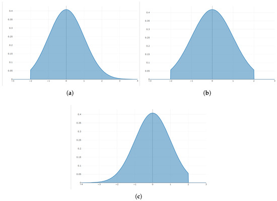
Figure 1.
Truncation normal distribution: (a) Left-truncated; (b) double-truncated; (c) right-truncated.
2.1. Statistical Characteristics of Left-Truncated Normal Distribution Data
Let and represent the probability density function (pdf) and cumulative distribution function (cdf) of the unconstrained distribution with parameters , and abbreviate them to , , respectively. Then, the pdf of X, given the restriction that it is truncated at , is
Assuming that X is a quality characteristic and follows a normal distribution, we denote it as . Then, the pdf of the truncated normal distribution is
Let be the standardized point of truncation.
Then, the k-th moment of the truncated distribution at the point of truncation is
Let be the pdf of the standard normal distribution, and be the cdf of the standard normal distribution. Then, as a function of , can be rewritten as
Here, it can be easily verified that .
Let the k-th moment about 0 of the truncated standard normal distribution be defined as follows in relation to the original complete distribution:
When and then 2, from Equation (6), we can obtain
For simplicity of the symbol, let
Here, the inverse Mills ratio function of the standard normal distribution is also referred to in this context as . Thus, Equation (7) follows
Let , and 2 in Equation (5), we get
2.2. Moment Estimators for Left-Truncated Normal Distribution Samples
Suppose is a sample set from a truncated normal distribution with n observations. A fundamental assumption in this study is that the observations are independently and identically distributed (i.i.d.). From the definition of moment estimation, Cohen [19] introduced the moment estimators for singly-truncated normal distribution samples as
where , .
From Equation (3), follows
To estimate in Equation (14), we should estimate and first. Eliminating the two equations in Equation (13), we get
and from the second equation of Equation (13), we have
Estimating by Equation (15) is a complicated task. A table of auxiliary functions for the estimator was presented in [19], which facilitates its use in the following application. If an equation-solving approach is employed, it can be implemented programmatically, as demonstrated in the pseudocode of Algorithm 1 below.
| Algorithm 1 Calculate the function |
|
3. and Indices Based on Singly-Truncated Normal Distribution Data
The process capability index is a key tool in statistical process control (SPC). It is a technique that is frequently used in modern industrial production to control and improve process capability. The process capability index provides a numerical quality standard for the ability of a process to produce a product that satisfies the factory’s pre-defined quality requirements, allowing the production department to improve a less capable process and raise the quality level. In the practical process capability analysis, two things must be confirmed. First, the data must be in a control state, and second, they must be examined to see if the data follow a normal distribution. If the data follow the normal distribution, the famous and indices can be used.
3.1. Classical and Indices
The index is suitable for cases where the process mean coincides with the target line, i.e., when the process does not shift. However, in actual manufacturing processes, the process usually fluctuates, and the mean value may shift from the target line; thus, an adjusted index, namely , is used. Table 1 provides the process capability evaluation reference for different and values.

Table 1.
CPI evaluation criteria [20].
3.1.1. Index
A index was defined as
where USL denotes upper specification limits, LSL denotes lower specification limits, and is the process standard deviation. The higher the value, the more sufficient the process capability; conversely, the lower the value, the less sufficient the process capability.
When a quality process is stationary and follows a Gaussian distribution, the estimator of the index is derived as
where is the standard deviation of the observations.
3.1.2. Index
The index was proposed to address the issue of process mean deviation from the target value, and it is defined as
The estimator of is
3.2. Modified and Indices
Assume that denotes a set of quality characteristics with n observations drawn from a stationary process and following a truncated normal distribution. Then, the original expectation and can be estimated using Equation (17):
where , , and is calculated using Equation (18).
The modified and indices based on the left-truncated normal distribution are defined as
and
where .
4. Confidence Interval Estimation of the Modified and Indices
The modified and indices may have significant inaccuracy due to the randomness of the sample collection; thus, the confidence interval of the two modified indices should also be investigated. It is very complicated to derive the distribution of and indices directly, but Guevara [21] proposed a simpler Monte Carlo approach for computing the process capability indices’ confidence intervals.
The bootstrap method was first proposed by Efron. Due to its simplicity and ease of use, among other things, it is frequently used in statistical inference and in estimating the distributions of unknown statistics. It is a traditional computer-intensive nonparametric method that is highly dependent on computers. It does not require knowing the sample distribution in advance. The fundamental principle of the bootstrap method is to create a new sample set by randomly selecting an equal number of samples from the observed sample set, and then computing the statistics for the new sample set. The aforementioned procedure is repeated a total of B times, resulting in a cluster of statistics. From the cluster, the empirical distribution of the statistics can be obtained, and point estimation, interval estimation, and hypothesis testing can be conducted using this distribution. The fundamental tenets of the bootstrap approach can be summed up as Table 2:
Table 2.
Bootstrap parameter estimation process.
4.1. Bootstrap Confidence Interval of and Indices
Assuming that is the quality set with n observations, from which n samples are drawn back a total of B times, and , denotes the set of samples drawn for the i-th time. The statistic , for each sample is the point estimate of the statistic ; thus, the estimated standard deviation of the statistic is s. The bootstrap confidence intervals of the statistic are defined as follows: The standard deviation of the estimate is given by ; therefore, the bootstrap confidence intervals for the statistic can be defined as in Equation (26).
where is the bootstrap variance of .
After resampling B times, we obtain two new datasets, and ; here, is the estimate of i-th sampling, and so is .
and
where is the variance estimation of the i-th sampling set.
Thus, the confidence intervals of and are defined as
where is the -quantile of the standard normal distribution, and are the means of and . Because both and asymptotically follow a normal distribution, their variances can be estimated using traditional variance estimation methods, as
4.2. Bootstrap Confidence Interval Estimation Procedure
To obtain the confidence interval of the investigated indices, the bootstrap method is used, and the procedure is simply presented as follows:
- Step 1.
- Collect the quality data for a certain character;
- Step 2.
- Use a histogram to check whether the data follow a left-truncated normal distribution; otherwise, recollect the quality data or estimate process capability using the traditional estimator.
- Step 3.
- When the observations follow a left-truncated normal distribution, calculate and using Equation (23);
- Step 4.
- Calculate the confidence interval for the process capability index based on the following scenarios: (1) normal distribution: calculate , ,,, respectively, and then compute the process capability under the normal distribution as follows:andrespectively; (2) truncated normal distribution: calculate , ,, using Equation (24), Equation (25), and Equation (26), respectively, and then the process capability under normal distribution is calculated as follows:andrespectively.
The above bootstrap confidence interval calculation steps were summarized in Figure 2.
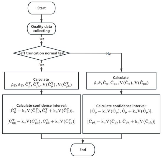
Figure 2.
Bootstrap confidence interval estimation procedure.
4.3. Computational Complexity of the Bootstrap Procedure
The scalability of the bootstrap method with respect to sample size (n) and resampling iterations (B) can be characterized as follows:
(1) Computational complexity with respect to sample size (n).
For each bootstrap iteration, the core operations include the following:
Resampling with replacement: Generate a bootstrap sample of size n from the original data, which requires time (linear in sample size).
Statistic recalculation: Compute the modified indices for the resampled data. Since the calculation of these indices involves the mean, standard deviation, and quantile estimates—all of which are operations—the total complexity per iteration is dominated by O(n).
(2) Computational complexity with respect to resampling iterations (B).
The bootstrap procedure repeats the above resampling and statistic-calculation steps B times. Thus, the overall computational complexity scales linearly with B, resulting in a total time complexity of for the entire bootstrap process.
5. Simulations and Numerical Analysis
5.1. Performance of and Indices
The following simulation experiments were conducted on the new indices and , and the results were compared with the true process capability values and in order to determine whether the new indices based on truncated sample theory can evaluate the process capability of the observed samples more accurately. The comparison also includes the and indices without taking truncation information into account, in order to more clearly show the efficacy of the suggested approach. Here, and are calculated in Formulas (24) and (25); and are defined in Formulas (19) and (21); and the estimating formulas for and are presented in Equations (20) and (22).
The comparison experiment was conducted from three aspects. First, by controlling the number of samples and the expectation and variance of the sample as a whole, and varying the position of the left-truncated point, we explored the impact of different cutoff point positions on the estimation of and . Second, by controlling the position of the left-truncated point and the expectation and variance of the sample as a whole, and letting the number of samples grow from small to large, we studied the impact of different sample sizes on the accuracy of the estimation results.
Since any normal distribution can be converted to a normal distribution, without loss of generality, the first two sets of simulation experiments use standard normal distribution observations, i.e., the population . The upper and lower specification lines are designed as , , respectively. Thus, the true process capability value of the sample is as follows:
All experiments were conducted on a PC using R software. All simulations were performed 10,000 times, with the average value being used as the final result in order to make the experimental results representative, given the random nature of sample collection.
Experiment 1. Set the observation sample size as , and let the value of the truncation point a change from to 3 in intervals of 0.1. Then, generate n random truncated samples using the rnormTrunc() function in the EnvStats package with parameter a as the truncation point, and estimate the values of , , , and using Equations (20), (22), (24), and (25), respectively. The results are shown in Figure 3 and Figure 4.
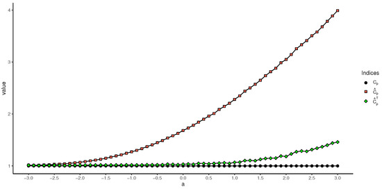
Figure 3.
Values of , , and based on different truncation values.
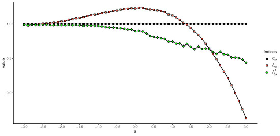
Figure 4.
Values of , , and based on different truncation values.
As can be seen in Figure 3 and Figure 4, the difference between and , as well as the difference between and , increases with the growing value of the truncation point, i.e., if the truncation information of the sample is not taken into account when calculating the process capability index for truncated samples, the final estimated result will be higher than the true value. For the newly proposed estimation method, the results of and slowly increase and drop, respectively. Nevertheless, both and outperform and . Moreover, on the left side of the symmetry axis , the difference between the estimates of and and the true values of and is very small, which implies that the proposed two process capability indices have a good chance of being applied when the truncation point is on the left side of the symmetry axis.
Experiment 2. Another issue we are concerned about is how the accuracy of the proposed index estimation varies with changes in the sample size. Understanding this issue will assist users in determining the appropriate sample size for practical applications. In this experiment, we compare the results of different estimations with the true values. To assess the sensitivity of the proposed method to sample size, the number of samples was increased progressively from 50 to 1000, and the truncation point was set to −2, −1, 0, 1, and 2, respectively. The simulated results are shown in Table 3 and Table 4.
Table 3.
and values under different sample sizes and truncation points.
Table 4.
and values under different sample sizes and truncation points.
Table 3 and Table 4 show that, when the cutoff value is controlled, the estimation results for and converge to the true value , whereas and also converge to the true value with the increase in the sample size. However, there is always a significant difference between the estimation results and , and the true values of and . This phenomenon can be further seen in Figure 5 and Figure 6. When the truncation value is set to , as can be seen, the and indices, which account for truncation information, outperform and in terms of estimating effect. Additionally, Table 3 and Table 4 show that when the truncated value increases, the estimation results for the index deteriorate; when the sample size is greater than 100, the estimation results for the newly proposed index are much closer to the true value. In addition, it can also be seen from Table 3 and Table 4 that, for the estimation of the index, the results of the index estimates become worse as the truncation value increases. However, the proposed index does not differ much from the true values when the sample size is greater than 100. For the performance of the index estimator, the performance of still outperforms that of .
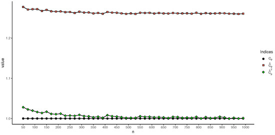
Figure 5.
Values of , , based on different sample sizes with truncation value .
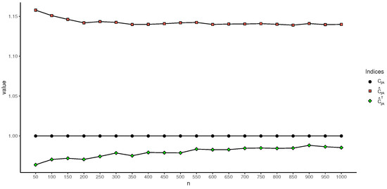
Figure 6.
Values of , , and based on different sample sizes with truncation value .
Experiment 3. To further investigate the absolute bias and root mean square error (RMSE) values of and under varying sample sizes, censoring rates, and mean shifts, Experiment 3 was designed. The absolute biases of the modified indices are presented in Figure 7 and Figure 8, while the RMSE results are shown in Figure 9 and Figure 10.
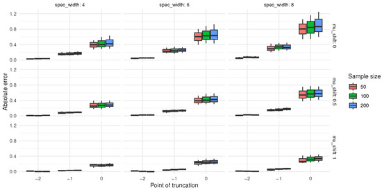
Figure 7.
The absolute deviation of .
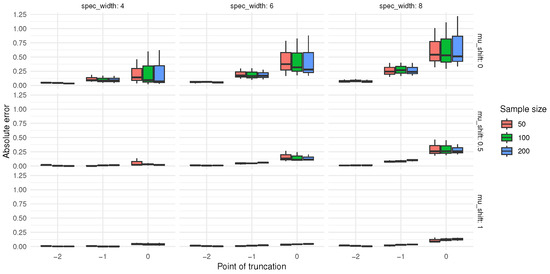
Figure 8.
The absolute deviation of .
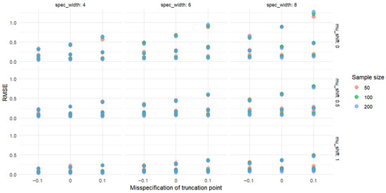
Figure 9.
The RMSE of .
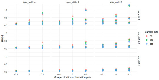
Figure 10.
The RMSE of .
Analysis of the data in Figure 7 and Figure 8 reveals certain patterns in the absolute biases of and under different sample sizes, censoring levels (indicated by the censoring point), and mean shifts. When the sample size is 50, under various censoring points, the absolute biases of both and generally decrease as the mean shift increases. Moreover, a larger censoring point (i.e., a lower degree of censoring) corresponds to greater absolute biases under the same mean shift. Similar trends are observed for a sample size of 100. Compared to the case with a sample size of 50, the absolute biases tend to decrease in some scenarios. When the sample size increases to 200, these patterns become more pronounced, and the absolute biases are further reduced in certain cases compared to those with a sample size of 100.
Overall, as the sample size increases, the absolute biases of and tend to decrease under the same censoring level and mean shift. For a fixed sample size, a lower degree of censoring (i.e., larger censoring point) generally leads to higher absolute bias. In addition, as the mean shift increases, the absolute biases of and mostly exhibit a declining trend. These findings indicate that sample size, censoring level, and mean shift all influence the absolute biases of and . In practical applications, these patterns can be utilized to optimize relevant operations or improve prediction accuracy.
As shown in Figure 9 and Figure 10, from the perspective of sample size, when the censoring level and mean shift are fixed, the RMSE values of both and generally exhibit a decreasing trend as the sample size increases from 50 to 200. For example, at a censoring point of −2 and a mean shift of 0, the RMSE of cpt decreases from 0.359639 (sample size 50) to 0.315073 (sample size 100), and further to 0.283292 (sample size 200); similarly, the RMSE of cpkt decreases from 0.375543 (sample size 50) to 0.329441 (sample size 100), and then to 0.287575 (sample size 200). These results indicate that larger sample sizes may contribute to reducing the RMSE values of and .
Regarding the censoring level, under the same sample size and mean shift, a larger censoring point (i.e., lower degree of censoring) tends to correspond to higher RMSE values for both and . For instance, at a sample size of 100 and a mean shift of 0, as the censoring point changes from −2 to 0, the RMSE of cpt increases from 0.315073 to 0.808805, and that of cpkt rises from 0.329441 to 0.688743.
In terms of the effect of mean shift, when the sample size and censoring level are fixed, the RMSE values of and mostly show a decreasing trend as the mean shift increases. Taking a sample size of 50 and a censoring point of −1 as an example, the RMSE of cpt decreases from 0.536742 (mean shift 0) to 0.363781 (mean shift 1), while the RMSE of cpkt drops from 0.520519 (mean shift 0) to 0.303010 (mean shift 1).
5.2. Bootstrap Confidence Interval for and Indices
One of the hotspots that researchers and quality managers are concerned about is the impact of shortened samples on process capability. According to Section 4.1, the truncation position can be found in a variety of places, and the sample size or truncation value will affect how accurately the process capability indices are estimated. The following simulation studies examine the interval estimation of the and indices under different parameter situations; the interval estimation of the and indices with different sample sizes and different truncation point locations is simulated below. This is done in order to further analyze the effect of samples containing truncation information on the interval estimation of the process capability indices.
The sample size n for the simulations that follow was changed from 50, 100, and 200 to 500, and the truncation values were selected with and . Using R software, random samples were created, the procedure was repeated 10,000 times, and the random seed was set to 123. The 95% SB confidence intervals of the and indices calculated by the traditional and proposed methods are shown in Table 5 and Table 6.
Table 5.
Simulation results of the SB confidence interval for the index under various process parameters with and true .
Table 6.
Simulation results of the SB confidence interval for the index for various process parameters with , true .
In Table 5 and Table 6, and denote the lower and upper confidence intervals of the estimated parameter . As can be seen from Table 5, the upper and lower confidence intervals of both and are larger than the true value , which indicates that when the truncation information exists, both and are overestimated. But this overestimation is inversely proportional to the change in sample size. Moreover, the index is overestimated to a much smaller extent than the index, and this tendency is reflected more clearly with the rightward shift of the truncation point. For example, when and , the confidence interval of is , and the confidence interval of is . At this point, the length of the confidence interval of is 0.012, which is smaller than the length of the confidence interval of , 0.014, and it is closer to the true value. However, when the sample size increases, the advantage of the confidence interval estimation results is quickly lost. For example, when , , ’s confidence interval is obviously better than ’s confidence interval , even though the lengths of their confidence intervals are the same.
If the sample is controlled so that the truncation position is gradually moved from −3 to 3, the confidence interval estimation advantage of the index becomes more evident than that of the index. For example, under the condition of a sample size of 50, when , the confidence interval of the index, , is far better than that of the index .
The same experiment becomes a little more complicated for the index. First of all, in the estimation of the index, will always be underestimated, while is overestimated when the truncation point is located on the left side of the symmetry axis. When the truncation point is moved to the right side of the symmetry axis, the estimation of the quickly becomes underestimated. This phenomenon can be seen in Figure 5 and Table 6.
Overall, the index estimate without considering truncation information may outperform the index only when the truncation point is located within . In the rest of the cases, the index, which considers sample truncation information, outperforms the index in confidence interval estimation.
Combining the results from Table 5 and Table 6, it is clear that the proposed new indices and outperform conventional estimation techniques in the majority of cases without taking into account sample truncation information in the confidence interval estimation. This shows that in the application of actual industrial production, we cannot ignore the existence of truncation information, especially for samples sent for testing in order to pass inspection. It is particularly noteworthy that both of the newly proposed indices show surprising accuracy when the truncation position of the sample is on the left side of the symmetry axis, for both point and interval estimation.
Building on the experiments above, we now discuss the bootstrap interval coverage of the true value under varying sample sizes, censoring rates, and mean shifts. The results are shown in Figure 5 and Figure 6
As shown in Figure 11 and Figure 12, from the perspective of sample size, when the censoring level and mean shift are held constant, the bootstrap interval coverage of the true value of both and generally exhibit a decreasing trend as the sample size increases from 50 to 200. For instance, at a censoring point of −2 and a mean shift of 0, the bootstrap interval coverage of the true value of decreases from 0.36 (sample size 50) to 0.32 (sample size 100), and further to 0.28 (sample size 200). Similarly, the bootstrap interval coverage of the true value of declines from 0.38 (sample size 50) to 0.33 (sample size 100), and then to 0.29 (sample size 200). These results suggest that larger sample sizes may help reduce the RMSE values of and .
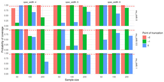
Figure 11.
The bootstrap interval coverage of the true value of . The red dashed line means a probability of 0.95.
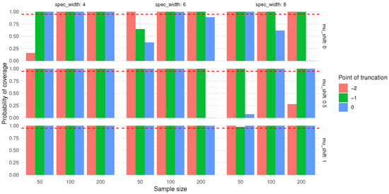
Figure 12.
The bootstrap interval coverage of the true value of . The red dashed line means a probability of 0.95.
With respect to the censoring level, under the same sample size and mean shift, a larger censoring point (i.e., lower degree of censoring) tends to correspond to higher RMSE values for both and . For example, at a sample size of 100 and a mean shift of 0, as the censoring point increases from −2 to 0, the RMSE of cpt rises from 0.32 to 0.81, and that of increases from 0.33 to 0.69.
Regarding the effect of mean shift, when the sample size and censoring level are fixed, the RMSE values of cpt and mostly show a declining trend with increasing mean shift. Taking a sample size of 50 and a censoring point of −1 as an example, the RMSE of cpt decreases from 0.54 (mean shift 0) to 0.36 (mean shift 1), while the RMSE of drops from 0.52 (mean shift 0) to 0.30 (mean shift 1).
6. Numerical Example
To illustrate the proposed method, this study uses information from a supplier who provided a new type of insulating material to an electronics company in Changsha. A central concern of the electronics company was the tensile strength of the flame-retardant material, which was required to be within the range of . The test data provided by the supplier contained a total of 80 samples, and the characteristics of the tensile strength values are shown in Table 7.
Table 7.
Tensile strength data for an electronics company from a supplier.
According to the manufacturer’s demands, we know that , , and the target value is . Firstly, the Q-Q plot method is used to test the data for normal distribution, and the test results are shown in Figure 13a. From the test results in Figure 13a, it can be seen that the data are basically distributed around the qq-line, indicating that the test data follow an approximately normal distribution.
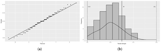
Figure 13.
Test for dataset: (a) Q-Q plot of the test data. (b) Histogram of the test data.
We create a histogram of the quality data in order to better examine the distribution pattern. The data for this quality characteristic clearly follow a left-truncated normal distribution, as shown in Figure 13. The truncation value was empirically set to 9.90 based on the inspection process.
6.1. Hypotheses Text for the Truncation Threshold
- Null hypothesis : Data are not left-truncated (complete data).
- Alternative hypothesis : Data are left-truncated.
6.2. Test Statistic
Let be the observed minimum value. Under , estimate distribution parameters:
Calculate the probability below c:
where is the standard normal cumulative distribution function.
Let Y be the actual number of observations below c. Since c is the minimum value, . Under :
Therefore,
When p is small and n is large, we can use the Poisson approximation:
6.3. Decision Rule
Given the significance level :
If is rejected, estimate the truncation point as .
6.4. Test Procedure
- Calculate sample statistics: .
- Compute z-score: .
- Calculate .
- Compute the binomial test p-value: .
- Compute the Poisson approximation p-value: .
- Compare the p-value with and make a decision.
6.5. Result
For the given tensile strength data (), let , following the truncation threshold test processing, we get Since , we accept , and suggest the data follow a left-truncated distribution.
6.6. Results
Point and interval estimation of the process capability index for this quality process is performed below. First, the expectation and variance of the quality data are calculated using the conventional method without considering the truncation information and the newly proposed method, respectively, and the results are obtained as follows:
Thus, the corresponding standard deviations are as follows:
The process capability index values calculated by conventional and modified methods can be obtained as follows:
According to Table 1, it can be seen that the value of process capability calculated using the conventional method belongs to the III level, i.e., the process capability is realized as general, which means that the technical management capability of this product is more reluctant and should be improved to the level II, while the value of the index of the revised method is 0.9509, which belongs to the IV level, which represents the insufficiency of the process capability, and should be diagnosed for the production process, and necessary measures should be taken to improve production. In terms of the performance of the index, the results calculated by both the conventional and revised methods show that the process capability of the product is seriously inadequate, and that the production line needs to be shut down and reorganized.
Based on the above conclusions, we constructed the corresponding confidence intervals for the process capability index to analyze the reliability of the conclusions. The 95% confidence intervals were calculated using the conventional method described in Equations (31) and (32) as follows:
The 95% confidence intervals were calculated using the modified method described in Equations (33) and (34) as follows:
According to the results of the above confidence interval estimation, the traditional method’s index result always indicates that it is generally adequate, while the improved method indicates that the process capability is insufficient, which feeds back to the actual activity, i.e., according to the result of the traditional index, the power company can accept the product, while according to the new method, the company should reject the product.
7. Conclusions
This study modifies two process capability evaluation indices, and , based on the truncation theory of statistical estimation for left-truncated samples, and then constructs the bootstrap confidence intervals for these two modified indices. To test the performance of the modified indices, we first performed Monte Carlo simulations of the point estimates of the proposed indices by setting different parameters and comparing them with the traditional estimation methods under the same conditions. The results demonstrate that the modified indices outperform the traditional methods in determining the process capability of left-truncated samples under various parameter conditions. Then, the accuracy and stability of the new technique are further validated by simulated tests using bootstrap confidence interval estimation.
Author Contributions
Conceptualization, Y.Y. and B.Y.; methodology, B.Y. and Y.Y.; software, B.Y. and P.L.; validation, B.Y., Y.Y. and P.L.; formal analysis, Y.Y.; resources, P.L.; data curation, B.Y.; writing—original draft preparation, B.Y.; writing—review and editing, Y.Y. and P.L.; visualization, B.Y.; supervision, P.L.; funding acquisition, Y.Y., B.Y. and P.L. All authors have read and agreed to the published version of the manuscript.
Funding
This research was funded by the National Natural Science Foundation of China (No. 12204540), the Project of the Social Science Popularization Base in Hunan Province (No. XJK22ZDJD35), and the Excellent Youth Project of the Hunan Provincial Education Department (No. 24B0865).
Data Availability Statement
The experimental datasets were randomly generated using R4.3.2 software, and the real datasets used in the test are available in the main text.
Conflicts of Interest
The authors declare no conflicts of interest.
References
- Borucka, A.; Kozłowski, E.; Antosz, K.; Parczewski, R. A New Approach to Production Process Capability Assessment for Non-Normal Data. Appl. Sci. 2023, 13, 6721. [Google Scholar] [CrossRef]
- Orosz, Á.; Varbanov, P.S.; Klemeš, J.J.; Friedler, F. Process synthesis considering sustainability for both normal and non-normal operations: P-graph approach. J. Clean. Prod. 2023, 414, 137696. [Google Scholar]
- Banihashemi, A.; Fallah Nezhad, M.S.; Amiri, A. Developing process-yield-based acceptance sampling plans for AR (1) auto-correlated process. Commun. Stat.-Simul. Comput. 2021, 52, 4230–4251. [Google Scholar] [CrossRef]
- Song, S.; Bai, Z.; Wei, H.; Xiao, Y. Copula-based methods for global sensitivity analysis with correlated random variables and stochastic processes under incomplete probability information. Aerosp. Sci. Technol. 2022, 129, 107811. [Google Scholar] [CrossRef]
- Chakraborty, A.K.; Chatterjee, M. Handbook of Multivariate Process Capability Indices; CRC Press: Boca Raton, FL, USA, 2021. [Google Scholar]
- Pearn, W.L.; Hung, H.N.; Peng, N.F.; Huang, C.Y. Testing process precision for truncated normal distributions. Microelectron. Reliab. 2007, 47, 2275–2281. [Google Scholar] [CrossRef]
- Yang, J.; Meng, F.; Huang, S.; Cui, Y. Process capability analysis for manufacturing processes based on the truncated data from supplier products. Int. J. Prod. Res. 2020, 58, 6235–6251. [Google Scholar] [CrossRef]
- Polansky, A.M.; Chou, Y.M.; Mason, R.L. Estimating Process Capability Indices for a Trltncated Distribution. Qual. Eng. 1998, 11, 257–265. [Google Scholar] [CrossRef]
- English, J.R.; Taylor, G.D. Process capability analysis—A robustness study. Int. J. Prod. Res. 1993, 31, 1621–1635. [Google Scholar] [CrossRef]
- Khadse, K.G.; Khadse, A.K. Assessing supplier’s process capability using truncated normal distribution data. J. Univ. Shanghai Sci. Technol. 2020, 52, 82–96. [Google Scholar]
- Lai, Y.W.; Chew, E.P. Gauge capability assessment for high-yield manufacturing processes with truncated distribution. Qual. Eng. 2000, 13, 203–210. [Google Scholar] [CrossRef]
- Tong, L.; Chen, J. Bootstrap confidence interval of the difference between two process capability indices. Int. J. Adv. Manuf. Technol. 2003, 21, 249–256. [Google Scholar] [CrossRef]
- Park, C.; Dey, S.; Ouyang, L.; Byun, J.H.; Leeds, M. Improved bootstrap confidence intervals for the process capability index Cpk. Commun.-Stat.-Simul. Comput. 2020, 49, 2583–2603. [Google Scholar] [CrossRef]
- Besseris, G.J. Evaluation of robust scale estimators for modified Weibull process capability indices and their bootstrap confidence intervals. Comput. Ind. Eng. 2018, 128, 135–149. [Google Scholar] [CrossRef]
- Fields, E.; Osorio, C.; Zhou, T. A Data-Driven Method for Reconstructing a Distribution from a Truncated Sample with an Application to Inferring Car-Sharing Demand. Transp. Sci. 2021, 55, 1–22. [Google Scholar] [CrossRef]
- Nie, G.Q.; Zhou, X.Y. Empirical Bayes test problem for the parameter of two-side truncated distribution families: In the case of NA samples. Breast Cancer Res. 2014, 41, 134–139. [Google Scholar]
- Gu, K.; Jia, X.Z.; You, H.L.; Liang, T. The yield estimation of semiconductor products based on truncated samples. Int. J. Metrol. Qual. Eng. 2014, 4, 215–220. [Google Scholar] [CrossRef]
- Kong, X.F.; He, Z.; Che, J.G. A judgement study on process capability of suppliers truncated treatment. Xitong Gongcheng Lilun Shijian/Syst. Eng. Theory Pract. 2008, 28, 75–80. [Google Scholar]
- Cohen, A.C. Truncated and Censored Samples: Theory and Applications; CRC Press: Boca Raton, FL, USA, 1991. [Google Scholar]
- Kane, V.E. Process capability indices. J. Qual. Technol. 1986, 18, 41–52. [Google Scholar] [CrossRef]
- Guevara, R.D.; Vargas, J.A. Comparison of process capability indices under autocorrelated data. Rev. Colomb. Estadíst. 2007, 30, 301–316. [Google Scholar]


Disclaimer/Publisher’s Note: The statements, opinions and data contained in all publications are solely those of the individual author(s) and contributor(s) and not of MDPI and/or the editor(s). MDPI and/or the editor(s) disclaim responsibility for any injury to people or property resulting from any ideas, methods, instructions or products referred to in the content. |
© 2025 by the authors. Licensee MDPI, Basel, Switzerland. This article is an open access article distributed under the terms and conditions of the Creative Commons Attribution (CC BY) license (https://creativecommons.org/licenses/by/4.0/).