New Logistic Family of Distributions: Applications to Reliability Engineering

Abstract

This study introduces a novel family of probability distributions, termed the Pi-Power Logistic-G family, constructed through the application of the Pi-power transformation technique. By employing the Weibull distribution as the baseline generator, a new and flexible model, the Pi-Power Logistic Weibull distribution, is formulated. Particular emphasis is given to this specific member of the family, which demonstrates a rich variety of hazard rate shapes, including J-shaped, reverse J-shaped, and monotonic increasing patterns, thereby highlighting its adaptability in modeling diverse types of lifetime data. The paper examines the fundamental properties of this distribution and applies the method of maximum likelihood estimation (MLE) to determine its parameters. A Monte Carlo simulation was performed to assess the performance of the estimation method, demonstrating that both Bias and mean square error decline as the sample size increases. The utility of the proposed distribution is further highlighted through its application to real-world engineering datasets. Using model selection metrics and goodness-of-fit tests, the results demonstrate that the proposed model outperforms existing alternatives. In addition, a Bayesian approach was used to estimate the parameters of both datasets, further extending the model’s applicability. The findings of this study have significant implications for the fields of reliability modeling, survival analysis, and distribution theory, enhancing methodologies and offering valuable theoretical insights.

1. Introduction

Probabilistic models are pivotal in representing and analyzing datasets across diverse practical applications. Classical distributions, such as log-normal, Lomax, exponential, Weibull, gamma, and beta, have been widely utilized; however, these models often fail to capture the complexity of certain datasets adequately. These traditional models struggle to accommodate varying degrees of skewness, kurtosis, and diverse hazard rate behaviors frequently encountered in empirical data. Consequently, there has been a growing interest in developing new families of distributions that offer enhanced flexibility, interpretability, and practical applicability.

To address these challenges, researchers have introduced various transformation-based approaches to generalize existing distributions. Among them, the T-X transformation [1] and the exponentiation technique have played foundational roles in the generation of flexible distribution families. For example, a new family of heavy-tailed (NFHT) distributions was proposed using the T-X transformation technique to analyze heavy-tailed datasets [2]. These methods have significantly broadened the modeling capacity of baseline distributions by introducing shape-controlling parameters.

In this study, we explored the $\pi$-power transformation (PPT), where $\pi$ is a constant, to develop a new and flexible probability model, initially presented by Lone and Jan [3] and later utilized by Kumar et al. [4]. This transformation enhances the base distribution by providing a unique blend of flexibility and skewness. This transformation allows for a smooth and continuous modification of the original distribution, enhancing its shape by introducing greater skewness and kurtosis, while still keeping the model analytically manageable. As a result, it offers both theoretical appeal and practical usefulness, especially for modeling complex real-world data. Moreover, this type of distribution has also shown good performance under the Bayesian framework.

Among the various distributions derived from the $\pi$-power transformation (PPT) framework, the $\pi$-exponentiated Weibull distribution has received particular attention due to its effectiveness in modeling lifetime and reliability data. The $\pi$-power transformation (PPT) framework is conceptually rooted in earlier transformation-based methodologies, particularly the alpha power transformation (APT), which has been widely adopted in probability theory, survival analysis, and reliability modeling. The APT technique has served as a foundation for constructing numerous generalized distribution families that offer improved flexibility in capturing complex data behaviors. For instance, the Alpha Power Weibull Quantile (APWQ) distribution and its associated family [5], along with the Alpha Power Exponentiated Weibull (APEW) distribution [6], were developed using APT techniques. Additionally, Mead et al. [6] investigated the mathematical properties of the APT family, filling gaps in earlier research, such as the work by Mahdavi and Kundu [7]. Several other notable families of distributions have been introduced using APT transformations. These include, but are not limited to, the Sine Alpha Power-G family [8], the Alpha Power Transformed Logistic (APTL) distribution [9], the Lomax distribution [10], the Pareto and inverse Pareto distributions [11,12], the Kumaraswamy distribution [13], the Alpha Power Topp–Leone Weibull distribution [14], and the Alpha Power of the Power Ailamujia distribution [15]. Moreover, some authors have proposed modifications to the APT transformation to develop novel families of distributions. For instance, Klakattawi and Aljuhani [16] introduced a new family of distributions by integrating both the T-X and APT transformation techniques. Alotaibi et al. [17] employed a weighted APT transformation to construct a new distribution. Additionally, Elbatal et al. [18] proposed an innovative alpha power transformation method that utilizes the quantile function alongside alternative cumulative distribution function (CDF) transformations.

Building on these developments, Lone and Jan [3] proposed the $\pi$-Exponentiated Transformed (PET) family, characterized by its CDF:

$$F\left(x\right)={\displaystyle \frac{{\pi }^{{\left\{T\left(x\right)\right\}}^{\delta }}-1}{\pi -1}},\delta >0,x\in \mathbb{R},$$

where $T\left(x\right)$ denotes the CDF of a base distribution. This transformation framework improves its flexibility and ability to capture skewness, thereby enabling more precise modeling of complex data structures.

Inspired by the PET framework, we introduce a novel method to develop a new family of distributions using a logit function of the CDF. This new family, termed the $\pi$-power logistic-G (PiPL-G) family, offers robustness and flexibility relative to conventional compound distributions. The PiPL-G family comprises two parameters that enable it to estimate its parameters and mathematical tractability effectively.

The $\pi$-power transformation used in the proposed model is mathematically distinct from other transformation techniques such as the alpha power transformation and the T-X family. In our formulation, $\pi$ is a known positive constant (e.g., $\pi =3.1416$), and the transformation is applied through a bounded, logistic-type exponent:

$$U(y;\rho ,\omega )={\displaystyle \frac{{\pi }^{\left(\frac{1-e^{-\rho y^{\omega }}}{1+e^{-\rho y^{\omega }}}\right)}-1}{\pi -1}}.$$

This design comes with several key benefits. First, the term $\left({\displaystyle \frac{1-e^{-\rho y^{\omega }}}{1+e^{-\rho y^{\omega }}}}\right)$ is always confined to the range $(0,1)$, which helps maintain numerical stability and ensures the distribution behaves smoothly. Second, keeping $\pi$ as a constant gives the model enough flexibility to represent a variety of hazard function shapes, including increasing, J-shaped, and reverse J-shaped, without the need for extra shape parameters. This not only prevents over-parameterization but also makes both the theoretical development and parameter estimation more straightforward.

In contrast, the alpha power transformation requires the estimation of an extra shape parameter, which can increase model complexity and reduce interpretability. Similarly, the T-X family involves complex transformations that may lack closed-form expressions for key functions, such as the density or quantile function, which complicates inference and application. The $\pi$-power transformation, therefore, offers a practical balance between model flexibility and computational tractability. Empirical results in this study support its utility, demonstrating good fit to real-world data across different applications while maintaining analytical and computational simplicity.

In reliability engineering, effectively modeling lifetime data is crucial for understanding failure mechanisms and predicting product reliability. The Weibull distribution, long regarded as a cornerstone in reliability theory, has been extensively employed to analyze such data. By integrating the PiPL-G framework, we provide an enhanced Weibull distribution that can capture diverse failure rates and survival probabilities with improved precision. This makes it particularly well suited for studying datasets involving accelerated life testing, stress–strength models, and warranty analysis. Among its members, the Weibull distribution stands out due to its prominence in reliability theory and life testing [19,20]. Integrating the PiPL-G framework further refines the Weibull distribution, aligning it with the unique features of various applications.

Our proposed PiPL-G family exhibits excellent flexibility for handling reliability engineering data, especially in cases where traditional models fail to accommodate complex failure patterns. For example, we have demonstrated the application of the PiPL-Weibull distribution in analyzing datasets with non-monotonic hazard rates and varying skewness levels. These features are essential for accurately assessing the reliability of systems and components in industries such as aerospace, manufacturing, and energy. Additionally, we applied our model to a real-world engineering dataset using a Bayesian approach, further enhancing its scope and demonstrating its practical utility. For Bayesian inference, we utilized Hamiltonian Monte Carlo (HMC), which is more efficient than Gibbs sampling and Metropolis–Hastings, implementing it through the rstan package in R version 4.4.3.

The proposed PiPL-G family builds upon existing reliability models by providing enhanced flexibility and adaptability to capture complex data behaviors commonly encountered in practice. Its ability to represent diverse hazard shapes and distributional features offers practitioners a more refined and versatile tool for modeling lifetime and survival data.

The rest of this paper is organized as follows: Section 2 introduces the PiPL-G family, while Section 3 presents the PiPL-Weibull distribution. Section 4 presents the mathematical and statistical properties, and Section 5 covers statistical inferences. Finally, Section 6, Section 7 and Section 8 present simulation experiments, applications, and conclusions, respectively.

2. Development of PiPL-G Family of Distributions

Here, we have developed a new distribution family. Let Y be a random variable; then the CDF of the PiPL-G family can be expressed as

$$U(y;\xi )={\displaystyle \frac{{\pi }^{\left(\frac{D(y;\xi )}{1+\overline{D}(y;\xi )}\right)}-1}{\pi -1}};y\in \mathbb{R}.$$

(1)

where $D(y;\xi )$ represents the CDF of any continuous baseline distribution with parameter space $\xi$, and $\pi$ is a constant ($3.1416$). Similarly, the probability density function (PDF) of PiPL-G can be expressed as

$$u(y;\xi )={\displaystyle \frac{(log\pi )}{\pi -1}}{\displaystyle \frac{2d(y;\xi )}{{\left[1+\overline{D}(y;\xi )\right]}^2}}{\pi }^{\left({\displaystyle \frac{D(y;\xi )}{1+\overline{D}(y;\xi )}}\right)};y\in \mathbb{R}.$$

(2)

Here, $D(y;\xi )$ refers to the CDF of any continuous baseline distribution, and $\overline{D}(y;\xi )$ represents a reliability function of the base distribution.

Now the reliability function R of the suggested family is computed using the CDF defined in (1), and can be expressed as

$$R(y;\xi )=1-{\displaystyle \frac{{\pi }^{\left(\frac{D(y;\xi )}{1+\overline{D}(y;\xi )}\right)}-1}{\pi -1}};y\in \mathbb{R}.$$

Linear Transformation of the PiPL-G Distribution

The CDF given in Equation (1) can be expanded into linear form using the exponential series expansion:

$$a^x=e^{xlna}=\sum _{n=0}^{\infty }{\displaystyle \frac{{(xlna)}^n}{n!}};-\infty <x<\infty ,$$

and we can express the CDF as

$$U(y;\xi )={\displaystyle \frac{1}{\pi -1}}\sum _{i=0}^{\infty }{\displaystyle \frac{{(log\pi )}^i}{i!}}{\left[D(y;\xi )\right]}^i{\left(1+\overline{D}(y;\xi )\right)}^{-i}-{\displaystyle \frac{1}{\pi -1}},i<0.$$

Again, by applying the negative binomial series

$${(1-x)}^{-m}=\sum _{n=0}^{\infty }\left({\displaystyle \genfrac{}{}{0pt}{}{m+n-1}{n}}\right)x^n;\left|x\right|\le 1,m<0,$$

we can write

$$U(y;\xi )={\displaystyle \frac{1}{\pi -1}}\sum _{i=0}^{\infty }\sum _{j=0}^{\infty }{(-1)}^j{\displaystyle \frac{{(log\pi )}^i}{i!}}\left({\displaystyle \genfrac{}{}{0pt}{}{i+j-1}{j}}\right){\left(1-D(y;\xi )\right)}^j{\left\{D(y;\xi )\right\}}^i-{\displaystyle \frac{1}{\pi -1}}.$$

Further, using the generalized binomial theorem

$${(1-x)}^m=\sum _{n=0}^{\infty }{(-1)}^n\left({\displaystyle \genfrac{}{}{0pt}{}{m}{n}}\right)x^n;\left|x\right|<1,$$

we obtain the linear form of the CDF as

$$U(y;\xi )={\displaystyle \frac{1}{\pi -1}}\sum _{i=0}^{\infty }\sum _{j=0}^{\infty }\sum _{k=0}^{\infty }{\left(-1\right)}^{j+k}{\displaystyle \frac{{\left(log\pi \right)}^i}{i!}}\left({\displaystyle \genfrac{}{}{0pt}{}{i+j-1}{j}}\right)\left({\displaystyle \genfrac{}{}{0pt}{}{j}{k}}\right)D^{i+k}(y;\xi )-{\displaystyle \frac{1}{\pi -1}}.$$

(3)

To verify the convergence of Equation (3), we analyzed the following terms separately:

• The term $D^{i+k}(y;\xi )\in [0,1]$ for all $y>0$, and for fixed y, this decays exponentially as $i+k\to \infty$.
• The coefficients ${\displaystyle \frac{{(log\pi )}^i}{i!}}$ decay faster than any polynomial growth in i, due to the factorial in the denominator.
• The binomial terms $\left({\displaystyle \genfrac{}{}{0pt}{}{i+j-1}{j}}\right)$ and $\left({\displaystyle \genfrac{}{}{0pt}{}{j}{k}}\right)$ grow polynomially, which is dominated by the exponential decay of ${\displaystyle \frac{{(log\pi )}^i}{i!}}$ and $D^{i+k}(y;\xi )$.
• The alternating sign ${(-1)}^{j+k}$ introduces cancellation, enhancing convergence.

Thus, the series defining $U(y;\xi )$ is absolutely convergent for all valid CDFs $D(y;\xi )$, provided $\pi >1$. This ensures the validity of the series expansion and its use in modeling.

Taking the derivative of Equation (3) with respect to y yields the linear form of the PDF, given by

$$u(y;\xi )=\sum _{i=0}^{\infty }\sum _{j=0}^{\infty }\sum _{k=0}^{\infty }{\Delta }_{ijk}{D}^{i+k-1}(y;\xi )d(y;\xi ),$$

where

$${\Delta }_{ijk}={\displaystyle \frac{{\left(-1\right)}^{j+k}}{\pi -1}}{\displaystyle \frac{\left(i+k\right){\left(log\pi \right)}^i}{i!}}\left({\displaystyle \genfrac{}{}{0pt}{}{i+j-1}{j}}\right)\left({\displaystyle \genfrac{}{}{0pt}{}{j}{k}}\right).$$

3. Pi-Power Logistic Weibull (PiPLW) Distribution

Let Y be a positive random variable that follows a Weibull distribution. The cumulative distribution function and probability density function of the Weibull distribution are expressed as

$$D(y;\rho ,\omega )=1-e^{-\rho y^{\omega }},\rho ,\omega >0,y>0.$$

(4)

$$d(y;\rho ,\omega )=\rho \omega y^{\omega -1}{e}^{-\rho y^{\omega }}.$$

(5)

By substituting Equation (4) as the base distribution into the CDF (1), we define a new distribution called the PiPLW distribution. Its CDF is expressed as

$$U(y;\rho ,\omega )={\displaystyle \frac{{\pi }^{\left(\frac{1-e^{-\rho y^{\omega }}}{1+e^{-\rho y^{\omega }}}\right)}-1}{\pi -1}},\rho ,\omega >0,y>0.$$

(6)

The parameters $\rho$ and $\omega$ govern the shape and scale of the distribution in ways particularly relevant to engineering reliability analysis:

• The parameter $\rho >0$ serves as a scale parameter, influencing the intensity of the failure rate. Higher values of $\rho$ shift the distribution toward shorter lifespans (left-skewed), indicating quicker degradation or early failures. Conversely, lower values of $\rho$ extend the distribution toward longer lifetimes, implying greater reliability. Thus, $\rho$ is inversely related to the system’s reliability—smaller $\rho$ values correspond to higher reliability.
• The parameter $\omega >0$ shapes the hazard function, enabling the model to accommodate various failure patterns, such as increasing, decreasing, or bathtub-shaped hazard rates.
• The parameter $\pi =3.1416$ serves as a distortion control factor, shaping the tail behavior of the distribution and expanding its adaptability to accommodate varied data patterns.

The corresponding PDF of the PiPLW distribution is derived using Equation (6) as

$$u(y;\rho ,\omega )={\displaystyle \frac{2\rho \omega (log\pi )}{\pi -1}}{\pi }^{\left({\displaystyle \frac{1-e^{-\rho y^{\omega }}}{1+e^{-\rho y^{\omega }}}}\right)}{\displaystyle \frac{y^{\omega -1}{e}^{-\rho y^{\omega }}}{{\left(1+e^{-\rho y^{\omega }}\right)}^2}},y>0.$$

(7)

Some important functions of the PiPLW distribution, such as the hazard rate function (HRF) and reliability function, are as follows:

$$h(y;\rho ,\omega )={\displaystyle \frac{2\rho \omega (log\pi )}{\pi -1}}{\pi }^{\left({\displaystyle \frac{1-e^{-\rho y^{\omega }}}{1+e^{-\rho y^{\omega }}}}\right)}{\displaystyle \frac{y^{\omega -1}{e}^{-\rho y^{\omega }}}{{\left(1+e^{-\rho y^{\omega }}\right)}^2}}{\left[1-{\displaystyle \frac{1}{\pi -1}}\left\{{\pi }^{\left({\displaystyle \frac{1-e^{-\rho y^{\omega }}}{1+e^{-\rho y^{\omega }}}}\right)}-1\right\}\right]}^{-1},y>0.$$

$$R(y;\rho ,\omega )=1-\left\{{\displaystyle \frac{{\pi }^{\left(\frac{1-e^{-\rho y^{\omega }}}{1+e^{-\rho y^{\omega }}}\right)}-1}{\pi -1}}\right\},y>0.$$

Qunatile Function (QF) for the PiPLW Distribution

The QF for the PiPLW distribution is obtained by inverting Equation (6) and is given as

$$Q_Y(u;\rho ,\omega )={\left[-{\displaystyle \frac{1}{\rho }}log\left({\displaystyle \frac{log\left(\pi \right)-log\left(u(\pi -1)+1\right)}{log\left(\pi \right)+log\left(u(\pi -1)+1\right)}}\right)\right]}^{1/\omega },0<u<1.$$

(8)

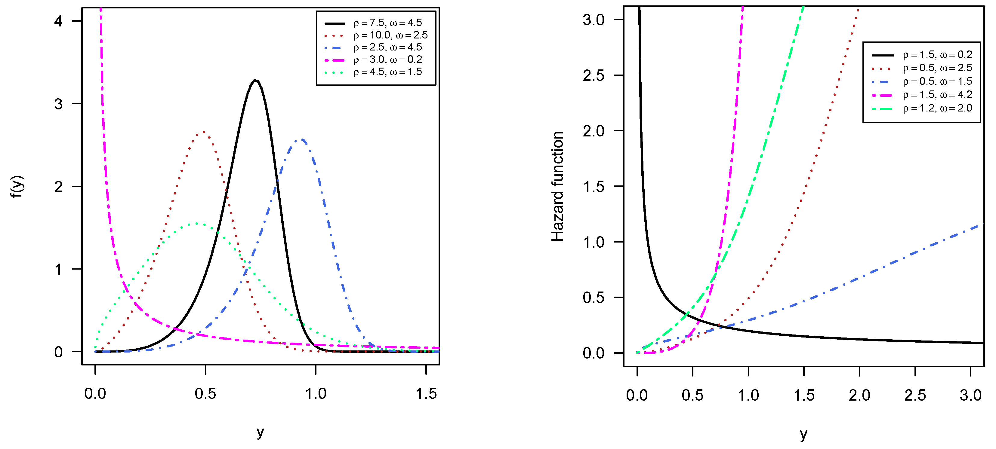
The PiPLW distribution exhibits various shapes in its PDF, including symmetric, right-skewed, left-skewed, or decreasing forms. Figure 1 (left) illustrates these variations. The HRF can take forms such as increasing, J-shaped, or reverse J-shaped, as shown in Figure 1 (right).

4. Some Important Properties of (PiPLW) Distribution

4.1. The PiPLW Distribution in Linear Form

Through further mathematical manipulation of Equation (7), the PDF of the PiPLW distribution can be expressed in a linearized form as

$$u(y;\rho ,\omega )=\sum _{i=0}^{\infty }\sum _{j=0}^{\infty }\sum _{k=0}^{\infty }\sum _{l=0}^{\infty }{\Delta }_{ijkl}^{*}{y}^{\omega -1}{e}^{-(l+1)\rho y^{\omega }},$$

where the coefficient ${\Delta }_{ijkl}^{*}$ is defined as

$${\Delta }_{ijkl}^{*}=\rho \omega {(-1)}^l{\Delta }_{ijk}\left({\displaystyle \genfrac{}{}{0pt}{}{i+k-1}{l}}\right).$$

4.2. Moments

Moments are important statistical tools for the study of a probability model. The $r^{th}$ moment from the origin of the PiPLW distribution can be obtained as

$$\begin{array}{cc}\hfill E\left[Y^r\right]& =\sum _{i=0}^{\infty }\sum _{l=0}^{\infty }\sum _{k=0}^{\infty }\sum _{j=0}^{\infty }{\Delta }_{ijkl}^{*}\underset{0}{\overset{\infty }{\int }}{y}^{\omega +r-1}{e}^{-\left(l+1\right)\rho y^{\omega }}dy\hfill \\ \hfill & =\sum _{i=0}^{\infty }\sum _{l=0}^{\infty }\sum _{k=0}^{\infty }\sum _{j=0}^{\infty }{\Delta }_{ijkl}^{*}{\displaystyle \frac{{\omega }^{-1}\mathsf{\Gamma }\left(\frac{r}{\omega }+1\right)}{{\left\{\left(l+1\right)\rho \right\}}^{\frac{r}{\omega }+1}}}.\hfill \end{array}$$

(9)

Mean and Variance of the PiPLW Distribution

Using Equation (9), we can calculate the mean, second moment, and variance as follows:

$$E\left[Y\right]=\mathrm{Mean}=\sum _{i=0}^{\infty }\sum _{l=0}^{\infty }\sum _{j=0}^{\infty }\sum _{k=0}^{\infty }{\Delta }_{ijkl}^{*}{\displaystyle \frac{{\omega }^{-1}\mathsf{\Gamma }\left(\frac{1}{\omega }+1\right)}{{\left\{\left(l+1\right)\rho \right\}}^{\frac{1}{\omega }+1}}}.$$

and

$$\begin{array}{ccc}\hfill V\left[Y\right]& =\hfill & \hfill =\sum _{i=0}^{\infty }\sum _{l=0}^{\infty }\sum _{k=0}^{\infty }\sum _{j=0}^{\infty }{\Delta }_{ijkl}^{*}{\displaystyle \frac{{\omega }^{-1}\mathsf{\Gamma }\left(\frac{2}{\omega }+1\right)}{{\left\{\left(l+1\right)\rho \right\}}^{\frac{2}{\omega }+1}}}-{\left[\sum _{i=0}^{\infty }\sum _{k=0}^{\infty }\sum _{k=0}^{\infty }\sum _{j=0}^{\infty }{\Delta }_{ijkl}^{*}{\displaystyle \frac{{\omega }^{-1}\mathsf{\Gamma }\left(\frac{1}{\omega }+1\right)}{{\left\{\left(l+1\right)\rho \right\}}^{\frac{1}{\omega }+1}}}\right]}^2.\end{array}$$

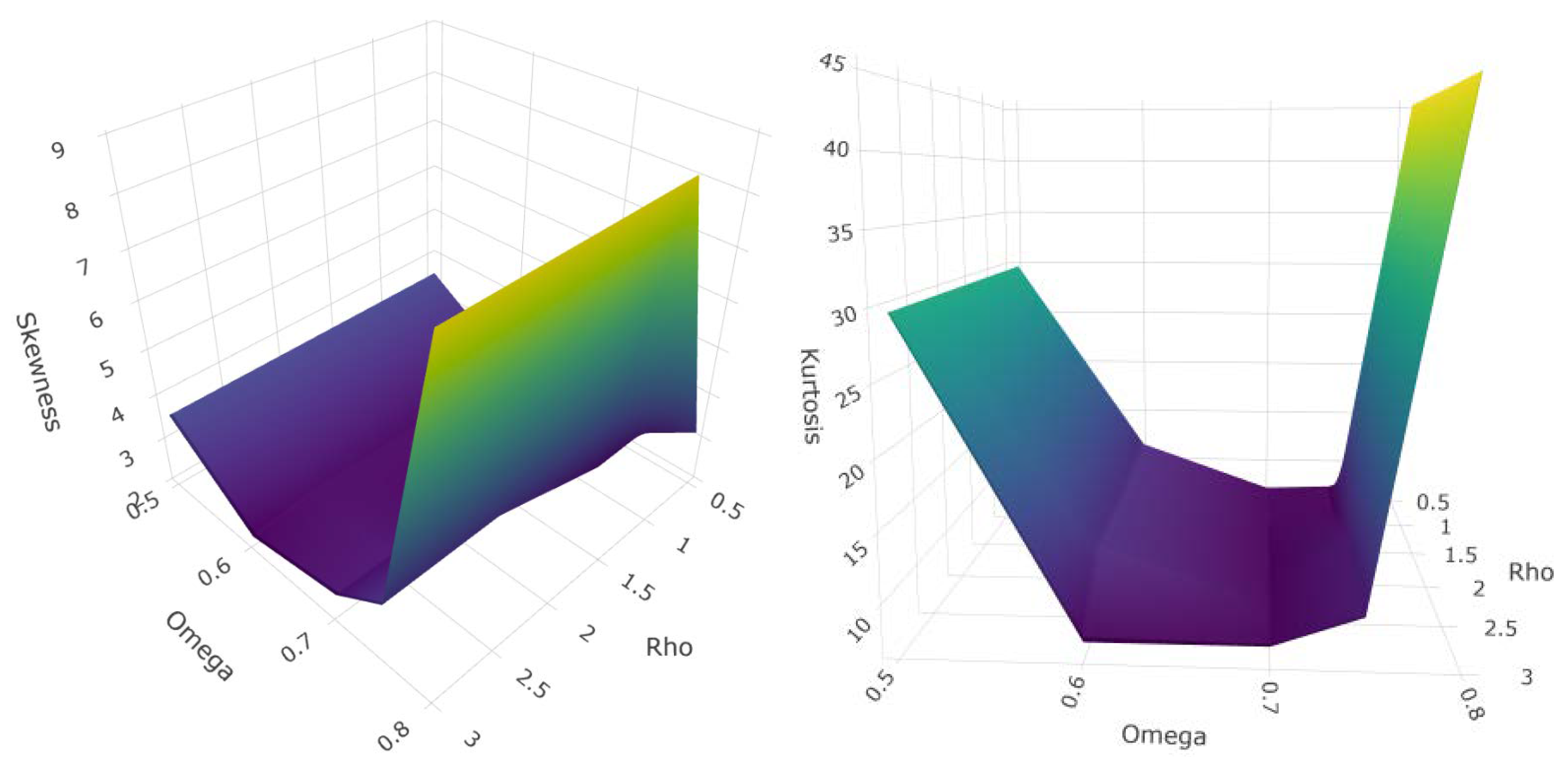
The numerical values of the mean, variance, skewness, and kurtosis presented in

Table 1. Numerical values of mean, variance, skewness, and kurtosis.

$\mathit{\rho }$	$\mathit{\omega }$	Mean	Variance	Skewness	Kurtosis
0.5	0.50	13.9128	955.5286	3.6150	29.674
1.0	0.60	4.9229	237.2861	2.3228	11.7335
2.0	0.70	0.8306	93.4530	2.1934	7.4200
2.5	0.75	−0.5029	62.4927	2.5171	7.6636
3.0	0.80	−1.5781	41.3941	3.2073	9.8521
3.5	0.90	−0.3738	0.1747	8.8566	44.6790
3.5	0.80	−0.1386	0.3193	3.2073	9.8521

were obtained by evaluating the moment expression given in Equation (9). All computations were performed using the base functions of the R programming environment. By varying the parameters of the distribution across a wide range of values, the corresponding moments were calculated to examine the statistical behavior of the model. The results demonstrate that the moment expression in Equation (9) is both well defined and convergent. Additionally, the variation in skewness and kurtosis across different parameter settings is visually represented in Figure 2, further highlighting the flexibility of the proposed distribution.

4.3. Moment-Generating Function (MGF)

We can also calculate different orders of moments using MGF, and it can be presented as

$$\begin{array}{cc}\hfill M_Y\left(t\right)& =\sum _{i=0}^{\infty }\sum _{k=0}^{\infty }\sum _{m=0}^{\infty }\sum _{l=0}^{\infty }\sum _{j=0}^{\infty }{\displaystyle \frac{t^m}{m!}}{\Delta }_{ijkl}^{*}\underset{0}{\overset{\infty }{\int }}{y}^{\omega +m-1}{e}^{-\left(l+1\right)\rho y^{\omega }}dy\hfill \\ & =\sum _{i=0}^{\infty }\sum _{k=0}^{\infty }\sum _{m=0}^{\infty }\sum _{l=0}^{\infty }\sum _{j=0}^{\infty }{\displaystyle \frac{t^m}{m!}}{\Delta }_{ijkl}^{*}{\displaystyle \frac{{\omega }^{-1}\mathsf{\Gamma }\left(\frac{m}{\omega }+1\right)}{{\left\{\left(l+1\right)\rho \right\}}^{\frac{m}{\omega }+1}}}.\hfill \end{array}$$

4.4. Characteristic Function

The characteristic function is particularly useful in probability theory and statistics for several reasons. One key advantage is that it simplifies the process of finding the distribution of sums of independent random variables. It is defined as ${\mathsf{\Phi }}_Y\left(t\right)=E\left(e^{vtY}\right)$, where t is a real number and v represents the imaginary unit.

$$\begin{array}{cc}\hfill {\mathsf{\Phi }}_Y\left(t\right)& =\sum _{i=0}^{\infty }\sum _{k=0}^{\infty }\sum _{m=0}^{\infty }\sum _{l=0}^{\infty }\sum _{j=0}^{\infty }{\displaystyle \frac{{\left(vt\right)}^m}{m!}}{\Delta }_{ijkl}^{*}\underset{0}{\overset{\infty }{\int }}{y}^{\omega +m-1}{e}^{-\left(l+1\right)\rho y^{\omega }}dy\hfill \\ & =\sum _{i=0}^{\infty }\sum _{k=0}^{\infty }\sum _{m=0}^{\infty }\sum _{l=0}^{\infty }\sum _{j=0}^{\infty }{\displaystyle \frac{{\left(vt\right)}^m}{m!}}{\Delta }_{ijkl}^{*}{\displaystyle \frac{{\omega }^{-1}\mathsf{\Gamma }\left(\frac{m}{\omega }+1\right)}{{\left\{\left(l+1\right)\rho \right\}}^{\frac{m}{\omega }+1}}}.\hfill \end{array}$$

4.5. Incomplete Moment

Incomplete moments are especially useful in fields such as economics and finance, where obtaining complete datasets is often challenging. For the PiPLW distribution, it can be expressed as

$$\begin{array}{cc}\hfill M_r\left(z\right)& =\sum _{i=0}^{\infty }\sum _{l=0}^{\infty }\sum _{j=0}^{\infty }\sum _{k=0}^{\infty }{\Delta }_{ijkl}^{*}\underset{0}{\overset{Z}{\int }}{y}^{\omega +r-1}{e}^{-\left(l+1\right)\rho y^{\omega }}dy\hfill \\ & =\sum _{i=0}^{\infty }\sum _{l=0}^{\infty }\sum _{j=0}^{\infty }\sum _{k=0}^{\infty }{\Delta }_{ijkl}^{*}{\displaystyle \frac{{\omega }^{-1}\left[\gamma \left(\frac{\omega +r}{\omega },\left(l+1\right)\rho z^{\omega }\right)\right]}{{\left\{\left(l+1\right)\rho \right\}}^{\frac{\omega +r}{\omega }}}},\hfill \end{array}$$

where $\gamma (.)$ represents the function of incomplete gamma.

4.6. Mean Residual Life

This function gives essential insights into the characteristics of lifespan distribution, making it a crucial concept for understanding reliability and survival analyses.

$$\begin{array}{cc}\hfill \overline{M\left(z\right)}& ={\displaystyle \frac{1}{F\left(z\right)}}\left[\mu -\sum _{i=0}^{\infty }\sum _{k=0}^{\infty }\sum _{j=0}^{\infty }\sum _{l=0}^{\infty }{\Delta }_{ijkl}^{*}\underset{0}{\overset{\infty }{\int }}{y}^{\omega -1}{e}^{-\left(l+1\right)\rho y^{\omega }}dy\right]-z\hfill \\ & ={\displaystyle \frac{1}{F\left(z\right)}}\left[\mu -\sum _{i=0}^{\infty }\sum _{k=0}^{\infty }\sum _{j=0}^{\infty }\sum _{l=0}^{\infty }{\Delta }_{ijkl}^{*}{\displaystyle \frac{{\omega }^{-1}\left[\gamma \left(\frac{\omega +1}{\omega },\left(l+1\right)\rho z^{\omega }\right)\right]}{{\left\{\left(l+1\right)\rho \right\}}^{\frac{\omega +1}{\omega }}}}\right]-z.\hfill \end{array}$$

4.7. Expression for System Reliability

In this subsection, we present the series and parallel system reliability as follows:

Series System:

Consider a system that has n independent items, where each item follows the PiPLW ($y;\rho ,\omega$) distribution. Further, let $T_i\sim PiPLW(y;\rho ,\omega )$ for $i=1,\dots ,n$, with the CDF $U(t_i;\rho ,\omega )$ and PDF $u(t_i;\rho ,\omega )$. The reliability function for a series of a linear system is

$$R_S\left(t\right)=\prod _{i=1}^n{R}_i\left(t\right)={\left[1-\left\{{\displaystyle \frac{1}{\pi -1}}\left\{{\pi }^{\left({\displaystyle \frac{1-e^{-\rho t^{\omega }}}{1+e^{-\rho t^{\omega }}}}\right)}-1\right\}\right\}\right]}^n;\rho ,\omega >0,t>0.$$

The CDF for a series system is given as

$$F_S\left(t\right)=1-\prod _{i=1}^n{R}_i\left(t\right)=1-{\left[1-\left\{{\displaystyle \frac{1}{\pi -1}}\left\{{\pi }^{\left({\displaystyle \frac{1-e^{-\rho t^{\omega }}}{1+e^{-\rho t^{\omega }}}}\right)}-1\right\}\right\}\right]}^n.$$

(10)

Taking the derivative of Equation (10), the PDF for the series system is obtained as

$$f_S\left(t\right)={\displaystyle \frac{d{F}_S\left(t\right)}{dt}}={\displaystyle \frac{2n\rho \omega (log\pi )}{\pi -1}}{\pi }^{\left({\displaystyle \frac{1-e^{-\rho t^{\omega }}}{1+e^{-\rho t^{\omega }}}}\right)}{\displaystyle \frac{t^{\omega -1}{e}^{-\rho t^{\omega }}}{{\left[1+e^{-\rho t^{\omega }}\right]}^2}}{\left[1-\left\{{\displaystyle \frac{1}{\pi -1}}\left\{{\pi }^{\left({\displaystyle \frac{1-e^{-\rho t^{\omega }}}{1+e^{-\rho t^{\omega }}}}\right)}-1\right\}\right\}\right]}^{n-1}.$$

The HRF for the series system is given by the ratio of the PDF to the reliability function:

$$h_S\left(t\right)={\displaystyle \frac{f_S\left(t\right)}{R_S\left(t\right)}}={\displaystyle \frac{2n\rho \omega (log\pi )}{\pi -1}}{\pi }^{\left({\displaystyle \frac{1-e^{-\rho t^{\omega }}}{1+e^{-\rho t^{\omega }}}}\right)}{\displaystyle \frac{t^{\omega -1}{e}^{-\rho t^{\omega }}}{{\left[1+e^{-\rho t^{\omega }}\right]}^2}}{\left[1-\left\{{\displaystyle \frac{1}{\pi -1}}\left\{{\pi }^{\left({\displaystyle \frac{1-e^{-\rho t^{\omega }}}{1+e^{-\rho t^{\omega }}}}\right)}-1\right\}\right\}\right]}^{-1}.$$

Parallel System:

Now, consider a system where n components operate in parallel, each following the $PiPLW(y;\rho ,\omega )$ distribution. Suppose $T_i(i=1,...,n)\sim PiPLW(y;\rho ,\omega )$, then for the parallel system, the reliability expression is

$$R_P\left(t\right)=1-\prod _{i=1}^n\left(1-R_i\left(t\right)\right)=1-{\left[{\displaystyle \frac{1}{\pi -1}}\left\{{\pi }^{\left({\displaystyle \frac{1-e^{-\rho t^{\omega }}}{1+e^{-\rho t^{\omega }}}}\right)}-1\right\}\right]}^n;\rho ,\omega >0,t>0.$$

The CDF for the parallel system is derived as

$$F_P\left(t\right)=1-R_P\left(t\right)={\left[{\displaystyle \frac{1}{\pi -1}}\left\{{\pi }^{\left({\displaystyle \frac{1-e^{-\rho t^{\omega }}}{1+e^{-\rho t^{\omega }}}}\right)}-1\right\}\right]}^n;\rho ,\omega >0,t>0.$$

(11)

Taking the derivative of Equation (11) for the parallel system, the PDF is expressed as

$$f_P\left(t\right)={\displaystyle \frac{2n\rho \omega (log\pi )}{\pi -1}}{\pi }^{\left({\displaystyle \frac{1-e^{-\rho t^{\omega }}}{1+e^{-\rho t^{\omega }}}}\right)}{\displaystyle \frac{t^{\omega -1}{e}^{-\rho t^{\omega }}}{{\left[1+e^{-\rho t^{\omega }}\right]}^2}}{\left[{\displaystyle \frac{1}{\pi -1}}\left\{{\pi }^{\left({\displaystyle \frac{1-e^{-\rho t^{\omega }}}{1+e^{-\rho t^{\omega }}}}\right)}-1\right\}\right]}^{n-1}.$$

Similarly, for a parallel system, the HRF can be expressed as

$$h_P\left(t\right)={\displaystyle \frac{\frac{2n\rho \omega (log\pi )}{\pi -1}{\pi }^{\left(\frac{1-e^{-\rho t^{\omega }}}{1+e^{-\rho t^{\omega }}}\right)}\frac{t^{\omega -1}{e}^{-\rho t^{\omega }}}{{\left[1+e^{-\rho t^{\omega }}\right]}^2}{\left[\frac{1}{\pi -1}\left\{{\pi }^{\left(\frac{1-e^{-\rho t^{\omega }}}{1+e^{-\rho t^{\omega }}}\right)}-1\right\}\right]}^{n-1}}{1-{\left[\frac{1}{\pi -1}\left\{{\pi }^{\left(\frac{1-e^{-\rho t^{\omega }}}{1+e^{-\rho t^{\omega }}}\right)}-1\right\}\right]}^n}}.$$

5. Statistical Inference

5.1. Parameter Estimation

Assume that $y_i$ ($i=1,\dots ,n$) are independent observations from the PiPLW distribution with parameters $\rho$ and $\omega$. The log-likelihood for this distribution can be expressed as

$$\begin{array}{cc}\hfill \ell (\underline{y};\rho ,\omega )& =nlog\left(2\rho \omega log\pi \right)-nlog(\pi -1)+(log\pi )\sum _{i=1}^n\left({\displaystyle \frac{1-e^{-\rho y_i^{\omega }}}{1+e^{-\rho y_i^{\omega }}}}\right)\hfill \\ \hfill & +(\omega -1)\sum _{i=1}^{n}log{y}_i-\rho \sum _{i=1}^n{y}_i^{\omega }-2\sum _{i=1}^{n}log\left(1+e^{-\rho y_i^{\omega }}\right).\hfill \end{array}$$

(12)

To estimate the parameters, the first-order derivatives of the log-likelihood function with respect to $\rho$ and $\omega$ are computed as follows:

$${\displaystyle \frac{\partial \ell }{\partial \rho }}={\displaystyle \frac{n}{\rho }}+(log\pi )\sum _{i=1}^n{\displaystyle \frac{2y_i^{\omega }{e}^{-\rho y_i^{\omega }}}{{\left(1+e^{-\rho y_i^{\omega }}\right)}^2}}-\sum _{i=1}^n{y}_i^{\omega }+2\sum _{i=1}^n{\displaystyle \frac{y_i^{\omega }{e}^{-\rho y_i^{\omega }}}{1+e^{-\rho y_i^{\omega }}}}.$$

$${\displaystyle \frac{\partial \ell }{\partial \omega }}={\displaystyle \frac{n}{\omega }}+(log\pi )\sum _{i=1}^n{\displaystyle \frac{2\rho y_i^{\omega }(log{y}_i)e^{-\rho y_i^{\omega }}}{{\left(1+e^{-\rho y_i^{\omega }}\right)}^2}}+\sum _{i=1}^{n}log{y}_i-\rho \sum _{i=1}^n{y}_i^{\omega }(log{y}_i)+2\sum _{i=1}^n{\displaystyle \frac{y_i^{\omega }(log{y}_i)\rho e^{-\rho y_i^{\omega }}}{1+e^{-\rho y_i^{\omega }}}}.$$

The MLE for $\rho$ and $\omega$ can be obtained by solving these nonlinear equations using appropriate computational tools.

5.2. Pivotal Quantity (PQ):

A PQ is a concept in statistics that plays a crucial role in hypothesis testing, confidence interval construction, and other inferential methods. Suppose $y_i$ ($i=1,\dots ,n$) follows a $PiPLW(y;\rho ,\omega )$ distribution. The PQ can be expressed as

$$-2\sum _{i=1}^{n}ln\left[U(y_i;\rho ,\omega )\right]\sim {\chi }_{2n}^2\Rightarrow -2\sum _{i=1}^{n}ln\left[1-U(y_i;\rho ,\omega )\right]\sim {\chi }_{2n}^2.$$

It is further defined as

$$\begin{array}{cc}\hfill PQ& =-2\sum _{i=1}^{n}ln\left[{\displaystyle \frac{1}{\pi -1}}\left\{{\pi }^{\left({\displaystyle \frac{1-e^{-\rho y_i^{\omega }}}{1+e^{-\rho y_i^{\omega }}}}\right)}-1\right\}\right]\sim {\chi }_{2n}^2,\hfill \\ & \Rightarrow PQ=-2\sum _{i=1}^{n}ln\left[1-{\displaystyle \frac{1}{\pi -1}}\left\{{\pi }^{\left({\displaystyle \frac{1-e^{-\rho y_i^{\omega }}}{1+e^{-\rho y_i^{\omega }}}}\right)}-1\right\}\right]\sim {\chi }_{2n}^2.\hfill \end{array}$$

Now consider $x_i$ ($i=1,\dots ,n$) and $y_i$ ($i=1,\dots ,m$), two independent random variables following the $PiPLW(x;\rho ,\omega )$ and $PiPLW(y;\rho ,\omega )$ distributions, with their CDFs $U(x_i;\rho ,\omega )$ and $U(y_i;\rho ,\omega )$, respectively. The relationships among pivotal quantities are

$${\displaystyle \frac{P{Q}_1}{P{Q}_2}}\sim Bet{a}_2(m,n),{\displaystyle \frac{P{Q}_1}{P{Q}_1+P{Q}_2}}\sim Bet{a}_1(m,n),\mathrm{and}{\displaystyle \frac{n}{m}}{\displaystyle \frac{P{Q}_1}{P{Q}_2}}\sim F(m,n),$$

where:

$$P{Q}_1=-2\sum _{i=1}^{n}ln\left[{\displaystyle \frac{1}{\pi -1}}\left\{{\pi }^{\left({\displaystyle \frac{1-e^{-\rho x_i^{\omega }}}{1+e^{-\rho x_i^{\omega }}}}\right)}-1\right\}\right]$$

and

$$P{Q}_2=-2\sum _{i=1}^{n}ln\left[{\displaystyle \frac{1}{\pi -1}}\left\{{\pi }^{\left({\displaystyle \frac{1-e^{-\rho y_i^{\omega }}}{1+e^{-\rho y_i^{\omega }}}}\right)}-1\right\}\right].$$

6. Simulation Experiment

This study employed the maxLik package in R version 4.4.3 [21] to generate random samples from the quantile function outlined in Equation (8), under different parameter configurations of the PiPLW distribution. MLEs were computed for these samples using the maxLik() function, which utilizes the BFGS optimization algorithm in R [22]. The purpose of this simulation was to evaluate the performance of parameter estimation.

The simulation involved sample sizes ranging from 150 to 400, increasing in increments of 50. Each scenario was replicated 1000 times to compute the Bias, mean square error (MSE), Probability Coverage (PC) (at 95% confidence interval), and Replication Convergence (RC).

Table 2. Simulation results for the MLEs of the PiPLW distribution for $\left(\rho =0.25,\omega =0.75\right)$.

n	Bias ($\mathit{\rho }$)	Bias ($\mathit{\omega }$)	MSE ($\mathit{\rho }$)	MSE ($\mathit{\omega }$)	PC ($\mathit{\rho }$)	PC ($\mathit{\omega }$)	RC
150	−0.0044	0.0090	0.0042	0.0029	0.940	0.961	1000
200	−0.0039	0.0068	0.0033	0.0022	0.934	0.956	1000
250	−0.0002	0.0036	0.0024	0.0016	0.962	0.964	1000
300	−0.0002	0.0037	0.0024	0.0015	0.931	0.933	1000
350	0.0000	0.0017	0.0018	0.0012	0.949	0.953	1000
400	0.0011	0.0011	0.0015	0.0010	0.957	0.954	1000

,

Table 3. Simulation results for the MLEs of the PiPLW distribution for $\left(\rho =0.5,\omega =0.5\right)$.

n	Bias ($\mathit{\rho }$)	Bias ($\mathit{\omega }$)	MSE ($\mathit{\rho }$)	MSE ($\mathit{\omega }$)	PC ($\mathit{\rho }$)	PC ($\mathit{\omega }$)	RC
150	−0.0049	0.0070	0.0046	0.0014	0.932	0.940	1000
200	−0.0019	0.0037	0.0030	0.0009	0.954	0.960	1000
250	−0.0004	0.0022	0.0023	0.0007	0.952	0.955	1000
300	0.0013	0.0018	0.0023	0.0007	0.935	0.943	1000
350	−0.0040	0.0034	0.0018	0.0005	0.942	0.955	1000
400	−0.0022	0.0021	0.0014	0.0004	0.962	0.962	1000

,

Table 4. Simulation results for the MLEs of the PiPLW distribution for $\left(\rho =0.75,\omega =1.5\right)$.

n	Bias ($\mathit{\rho }$)	Bias ($\mathit{\omega }$)	MSE ($\mathit{\rho }$)	MSE ($\mathit{\omega }$)	PC ($\mathit{\rho }$)	PC ($\mathit{\omega }$)	RC
150	0.0030	0.0100	0.0064	0.0121	0.950	0.940	1000
200	−0.0056	0.0143	0.0049	0.0093	0.943	0.941	1000
250	−0.0011	0.0087	0.0039	0.0071	0.945	0.950	1000
300	−0.0007	0.0067	0.0027	0.0049	0.959	0.966	1000
350	0.0001	0.0031	0.0027	0.0047	0.937	0.956	1000
400	−0.0033	0.0095	0.0021	0.0040	0.957	0.954	1000

,

Table 5. Simulation results for the MLEs of the PiPLW distribution for $\left(\rho =1.25,\omega =2.5\right)$.

n	Bias ($\mathit{\rho }$)	Bias ($\mathit{\omega }$)	MSE ($\mathit{\rho }$)	MSE ($\mathit{\omega }$)	PC ($\mathit{\rho }$)	PC ($\mathit{\omega }$)	RC
150	0.0023	0.0240	0.0095	0.0319	0.956	0.958	1000
200	0.0045	0.0212	0.0069	0.0240	0.952	0.952	1000
250	−0.0057	0.0180	0.0057	0.0194	0.951	0.953	1000
300	0.0001	0.0107	0.0048	0.0149	0.955	0.955	1000
350	−0.0006	0.0146	0.0041	0.0134	0.947	0.957	1000
400	−0.0027	0.0161	0.0036	0.0121	0.942	0.951	1000

,

Table 6. Simulation results for the MLEs of the PiPLW distribution for $\left(\rho =1.5,\omega =0.5\right)$.

n	Bias ($\mathit{\rho }$)	Bias ($\mathit{\omega }$)	MSE ($\mathit{\rho }$)	MSE ($\mathit{\omega }$)	PC ($\mathit{\rho }$)	PC ($\mathit{\omega }$)	RC
150	0.0045	0.0039	0.0109	0.0014	0.942	0.938	1000
200	−0.0011	0.0042	0.0082	0.0010	0.953	0.951	1000
250	0.0021	0.0022	0.0067	0.0007	0.958	0.956	1000
300	−0.0012	0.0032	0.0054	0.0006	0.953	0.954	1000
350	−0.0003	0.0025	0.0047	0.0005	0.955	0.955	1000
400	0.0016	0.0013	0.0042	0.0005	0.947	0.950	1000

,

Table 7. Simulation results for the MLEs of the PiPLW distribution for $\left(\rho =2.0,\omega =1.5\right)$.

n	Bias ($\mathit{\rho }$)	Bias ($\mathit{\omega }$)	MSE ($\mathit{\rho }$)	MSE ($\mathit{\omega }$)	PC ($\mathit{\rho }$)	PC ($\mathit{\omega }$)	RC
150	0.0076	0.0132	0.0155	0.0111	0.957	0.956	1000
200	0.0037	0.0146	0.0117	0.0086	0.952	0.954	1000
250	0.0019	0.0096	0.0089	0.0072	0.959	0.947	1000
300	0.0053	0.0072	0.0083	0.0060	0.932	0.942	1000
350	0.0012	0.0064	0.0069	0.0050	0.941	0.95	1000
400	−0.0001	0.0041	0.0057	0.0042	0.949	0.956	1000

,

Table 8. Simulation results for the MLEs of the PiPLW distribution for $\left(\rho =2.5,\omega =3.5\right)$.

n	Bias ($\mathit{\rho }$)	Bias ($\mathit{\omega }$)	MSE ($\mathit{\rho }$)	MSE ($\mathit{\omega }$)	PC ($\mathit{\rho }$)	PC ($\mathit{\omega }$)	RC
150	0.0132	0.0381	0.0215	0.0685	0.956	0.946	1000
200	0.0121	0.0361	0.0183	0.0463	0.938	0.961	1000
250	0.0044	0.0203	0.0140	0.0371	0.945	0.956	1000
300	0.0115	0.0171	0.0119	0.0311	0.943	0.957	1000
350	0.0085	0.0024	0.0096	0.0290	0.947	0.933	1000
400	0.0062	0.0096	0.0081	0.0235	0.951	0.944	1000

and

Table 9. Simulation results for the MLEs of the PiPLW distribution for $\left(\rho =3.5,\omega =2.5\right)$.

n	Bias ($\mathit{\rho }$)	Bias ($\mathit{\omega }$)	MSE ($\mathit{\rho }$)	MSE ($\mathit{\omega }$)	PC ($\mathit{\rho }$)	PC ($\mathit{\omega }$)	RC
150	0.0230	0.0270	0.0533	0.0329	0.938	0.947	1000
200	0.0157	0.0239	0.0361	0.0240	0.953	0.958	1000
250	0.0206	0.0154	0.0309	0.0196	0.941	0.942	1000
300	0.0091	0.0163	0.0228	0.0153	0.959	0.955	1000
350	0.0067	0.0142	0.0203	0.0131	0.947	0.956	1000
400	0.0200	0.0082	0.0188	0.0118	0.959	0.960	1000

summarize the values of Bias MSE, PC, and RC for different parameter configurations. These results confirm that the MLEs perform well in finite samples, with negligible Bias, decreasing MSE, and coverage probabilities consistently close to the nominal 95% level as the sample size increases. This supports the reliability of inference procedures based on the PiPLW distribution for moderate to large samples.

7. Application

This section presents the application of the PiPLW distribution to real-world datasets. A description of these datasets is provided below.

Dataset I:

This dataset corresponds to the breaking stress of 50 mm long carbon fibers, measured in GPa. This dataset has also been utilized in several studies, including those by Oguntunde et al. [23] and Sapkota and Kumar [24].

Dataset II:

This dataset illustrates the symmetric distribution of tensile strength measurements from 87 carbon fiber samples, as reported by Nichols and Padgett [25].

We used the Total Time on Test (TTT) plot to examine the pattern of failure over time (see Figure 3). The plot showed a concave curve lying above the reference line, which suggests an increasing failure rate.

7.1. Model Analysis (Classical Approach)

To evaluate the fit of the models to datasets I and II, several established goodness-of-fit statistics were used. The assessment involved calculating metrics such as the Akaike Information Criterion (AIC), log-likelihood value (−2logL), Hannan–Quinn Information Criterion (HQIC), and the Kolmogorov–Smirnov (KS) test, along with their associated p-values. All computations and visualizations were performed using R version 4.4.3 [22,26]. To benchmark the performance of the PiPLW model, comparisons were made with several alternative models, including the Kavya Manoharan-inverse Weibull (KMIW) [27], the Lindley Weibull (LW) [28], the alpha power exponential (APE) [7], as well as the inverse Weibull (IW), Weibull, alpha power inverse Pareto (APIP) [12], and Alpha Power Weibull Quantile (APWQ) [29].

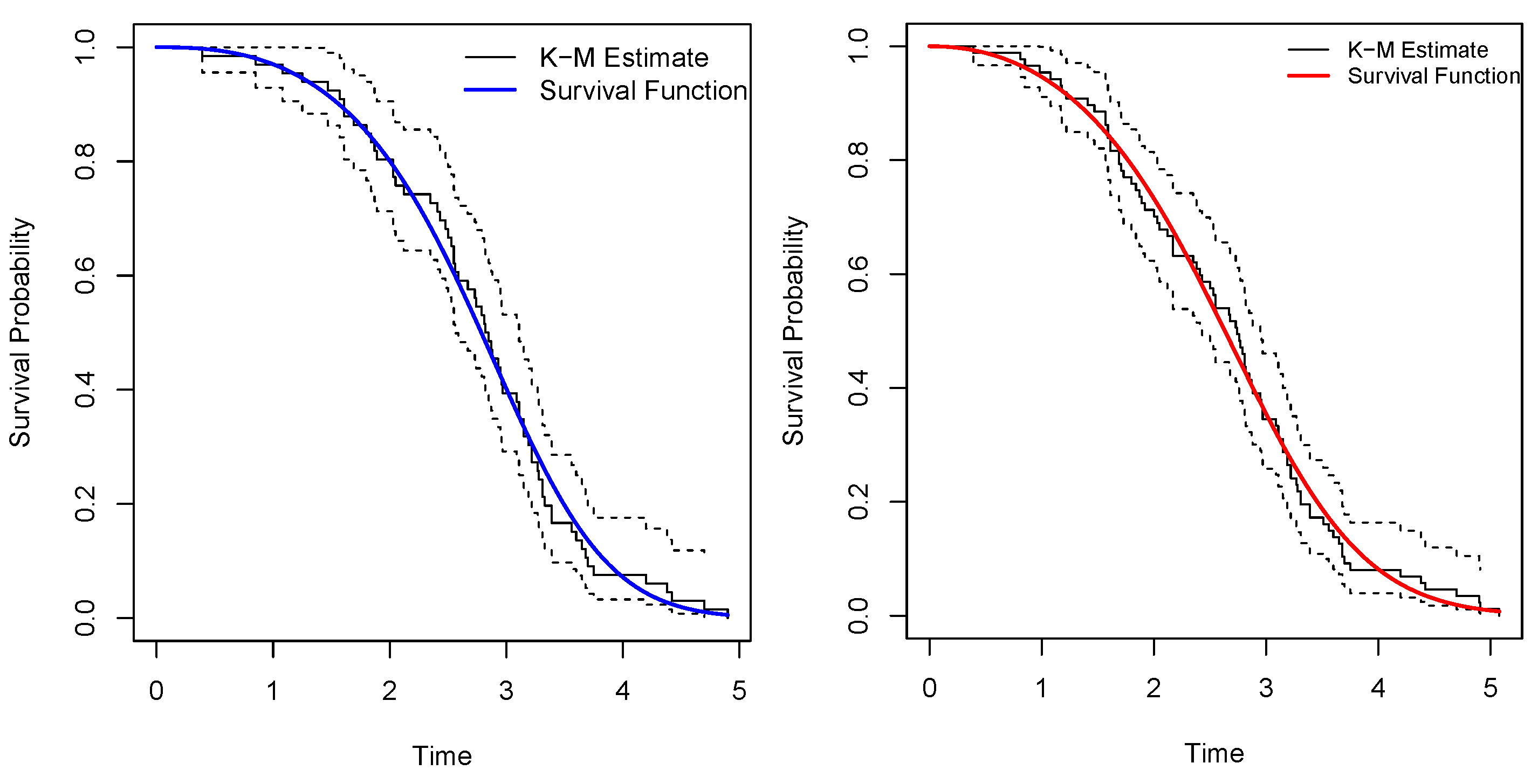
Figure 4 depicts the Kaplan–Meier estimator plots, which offer an approximation of the survival function for both datasets. The two dashed lines flanking the curves in the plots depict the confidence intervals (CIs) for the Kaplan–Meier estimates in Figure 4 (left panel for dataset I, right panel for dataset II).

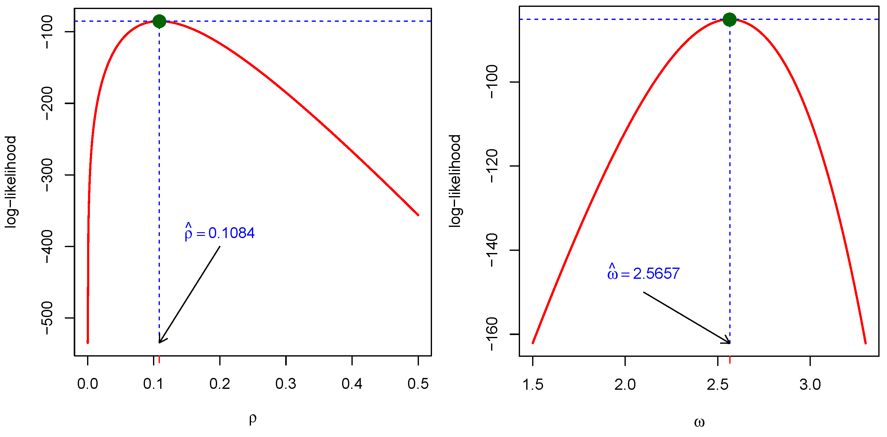
The MLEs of the parameters were obtained using the maxLik() function from the maxLik package in R, employing the BFGS optimization method. The initial values for the parameters were set to 0.5 for both parameters for both datasets, i.e., start = c(0.5, 0.5). Parameter (Par) estimates along with their standard errors (SEs) for dataset I are summarized in

Table 10. Parameter estimated through the MLE method for dataset I.

Distribution	Par	SE	Par	SE	Par	SE
PiPLW ($\rho ,\omega$)	0.1084	0.0369	2.5657	0.2663	–	–
KMIW ($\alpha ,\lambda$)	1.4705	0.1127	2.5576	0.2128	–	–
LW ($\alpha ,\beta ,\lambda$)	0.5870	0.3744	2.7796	0.4678	0.3629	0.4940
APE ($\alpha ,\lambda$)	156.1356	3.4252	0.8045	0.0535	–	–
IW ($\alpha ,\beta$)	1.6480	0.1226	3.2263	0.4193	–	–
Weibull ($\alpha ,\beta$)	0.0212	0.0091	3.4414	0.3302	–	–
APIP ($\delta ,\lambda$)	67.6438	4.1731	0.6837	0.0936	–	–
APWQ ($\alpha ,\beta ,\lambda$)	1.0000	0.9583	3.2951	0.1354	0.0255	0.0139

. Additionally, model selection criteria, including log-likelihood, HQIC, and AIC, BIC, along with goodness-of-fit measures such as the KS statistic and the corresponding p-values of dataset I, are presented in

Table 11. Model selection and goodness-of-fit statistics for dataset I.

Distribution	−2logL	AIC	HQIC	KS	p (KS)	CVM	p (CVM)	AD	p (AD)
PiPLW	170.2232	174.2232	175.9537	0.0703	0.9004	0.0524	0.8630	0.3373	0.9074
KMIW	240.7990	244.7990	246.5294	0.9634	0.0000	1.0889	0.0014	6.0555	0.0009
LW	171.0135	177.0135	179.6092	0.0735	0.8682	0.0671	0.7712	0.4037	0.8446
APE	201.2533	205.2533	206.9838	0.2075	0.0068	0.8826	0.0045	4.7910	0.0036
IW	242.3898	246.3898	248.1203	0.2303	0.0018	1.1562	0.0010	6.5040	0.0006
Weibull	172.1352	176.1352	177.8656	0.0823	0.7630	0.0836	0.6728	0.4858	0.7608
APIP	300.1459	304.1459	305.8764	0.4009	0.0000	3.0015	0.0000	14.7753	0.0000
APWQ	172.3341	178.3341	180.9299	0.0975	0.5577	0.1145	0.5195	0.6027	0.6448

. Likewise, Parameter (Par) estimates along with their standard errors (SEs) for dataset II are summarized in

Table 12. Parameters estimated through the MLE method for dataset II.

Distribution	Par	SE	Par	SE	Par	SE
PiPLW ($\rho ,\omega$)	0.1911	0.048	2.1299	0.1945	–	–
KMIW ($\alpha ,\lambda$)	1.5344	0.1078	2.3383	0.1646	–	–
LW ($\alpha ,\beta ,\lambda$)	0.3156	0.5714	2.7065	0.8544	1.7071	7.0748
APE ($\alpha ,\lambda$)	138.8604	119.5642	0.8309	0.0000	–	–
IW ($\alpha ,\beta$)	1.7282	0.1169	3.0157	0.3421	–	–
Weibull ($\alpha ,\beta$)	0.0439	0.0138	2.8913	0.2411	–	–
APIP ($\delta ,\lambda$)	93.5716	5.9844	0.5992	0.0721	–	–
APWQ ($\alpha ,\beta ,\lambda$)	1.0000	1.7004	2.8501	0.5491	0.0463	0.0503

. Similarly, model selection criteria, including log-likelihood, HQIC, and AIC, BIC, along with goodness-of-fit measures such as the KS statistic and the corresponding p-values of dataset II, are presented in

Table 13. Model selection and goodness-of-fit statistics for dataset II.

Distribution	−2logL	AIC	HQIC	KS	p (KS)	CVM	p (CVM)	AD	p (AD)
PiPLW	243.3537	247.3537	249.3396	0.0562	0.9464	0.0508	0.8726	0.3613	0.8858
KMIW	304.6385	308.6385	310.6244	0.9628	0.0000	0.9072	0.0039	5.0858	0.0026
LW	243.4470	249.1470	252.1258	0.0631	0.8794	0.0595	0.8182	0.3876	0.8606
APE	265.6065	269.6065	271.5924	0.1420	0.0600	0.5767	0.0253	3.4469	0.0164
IW	305.3344	309.3344	311.3203	0.1840	0.0055	0.8704	0.0048	5.2332	0.0022
Weibull	243.4833	247.4833	249.4692	0.0681	0.8145	0.0638	0.7914	0.3905	0.8577
APIP	386.6192	390.6192	392.6051	0.3753	0.0000	3.4150	0.0000	17.2266	0.0000
APWQ	243.5137	249.1137	252.0925	0.0727	0.7467	0.0683	0.7631	0.4025	0.8459

. To provide a clearer picture of parameter estimation, we plotted the profile log-likelihood plots in Figure 5 and Figure 6 for both datasets.

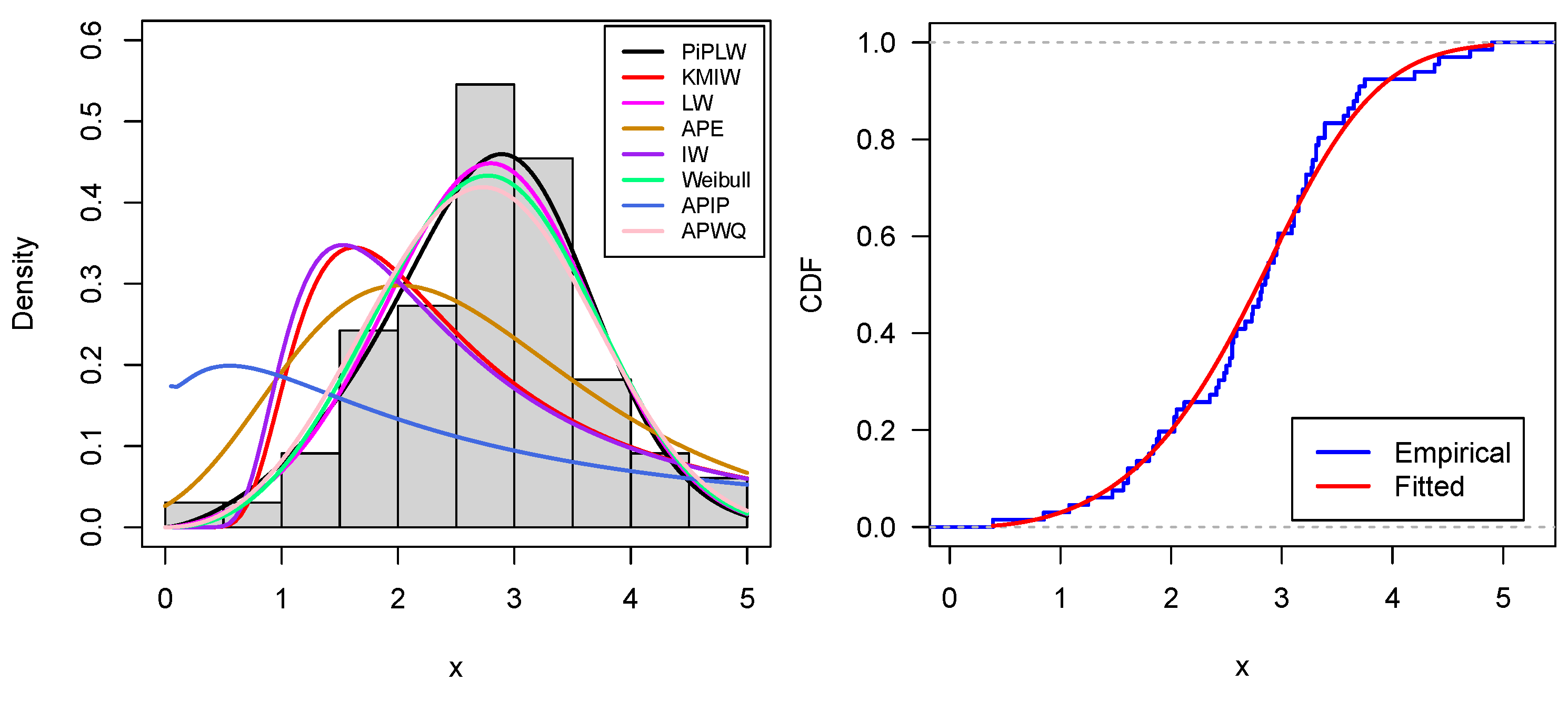
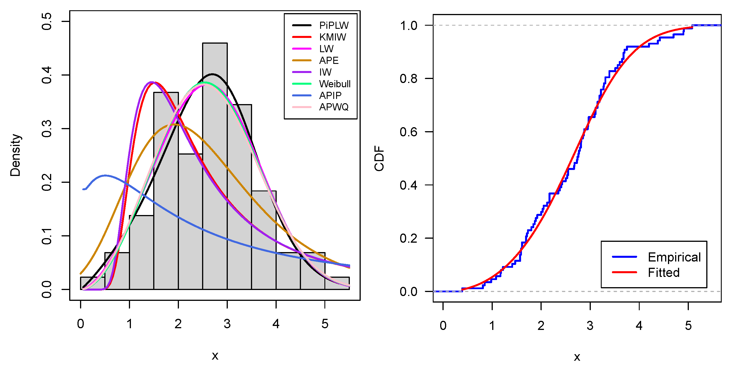
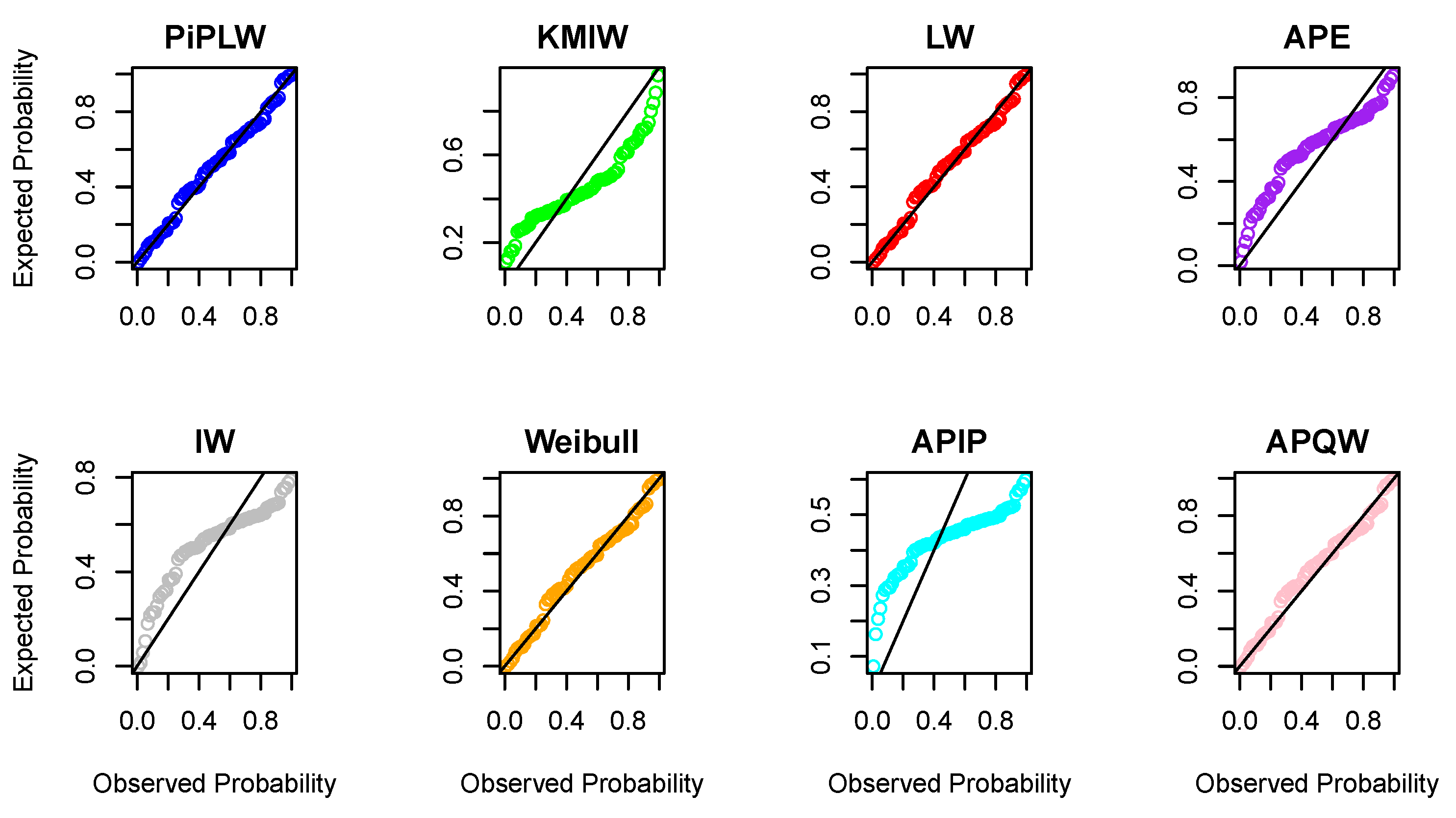
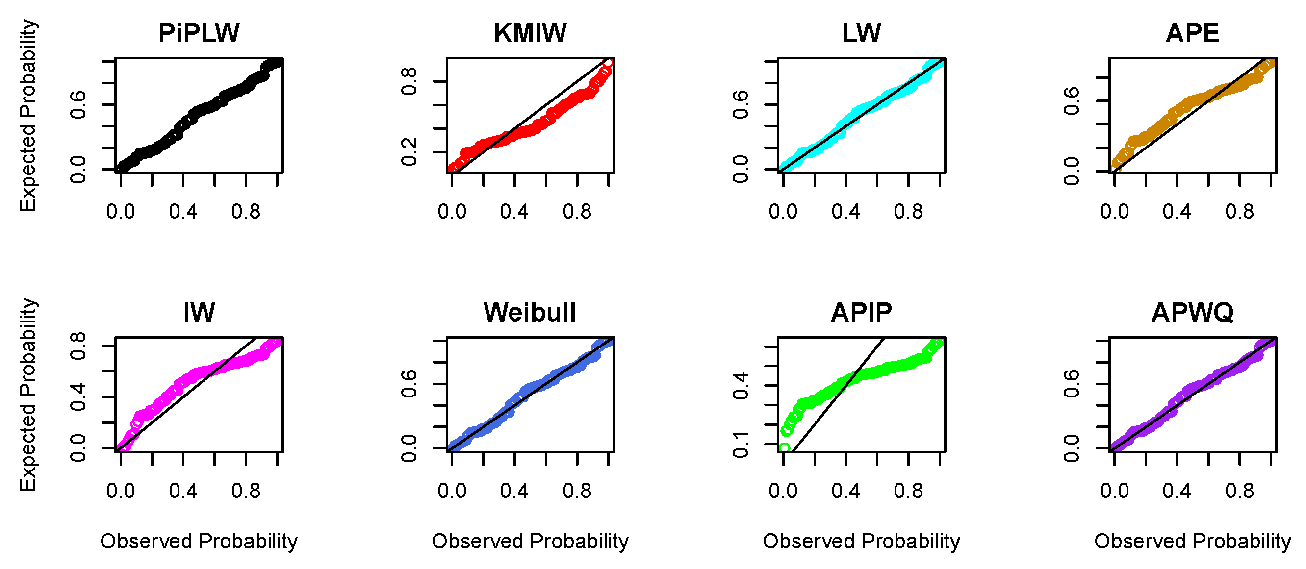
The results indicate that the PiPLW distribution consistently yielded lower values for model selection criteria in comparison to the KMIW, LW, APE, IW, Weibull, APIP, and APWQ distributions. These findings confirm the superior performance and greater flexibility of the PiPLW distribution in modeling real-world data. Furthermore, the fitted PDF and CDF presented in Figure 7 and Figure 8 visually support the conclusion that the PiPLW model provides a better fit than the competing models. The probability–probability (P–P) plots shown in Figure 9 and Figure 10 for both datasets further illustrate the superior fit of the proposed model.

7.2. Model Analysis (Bayesian Approach)

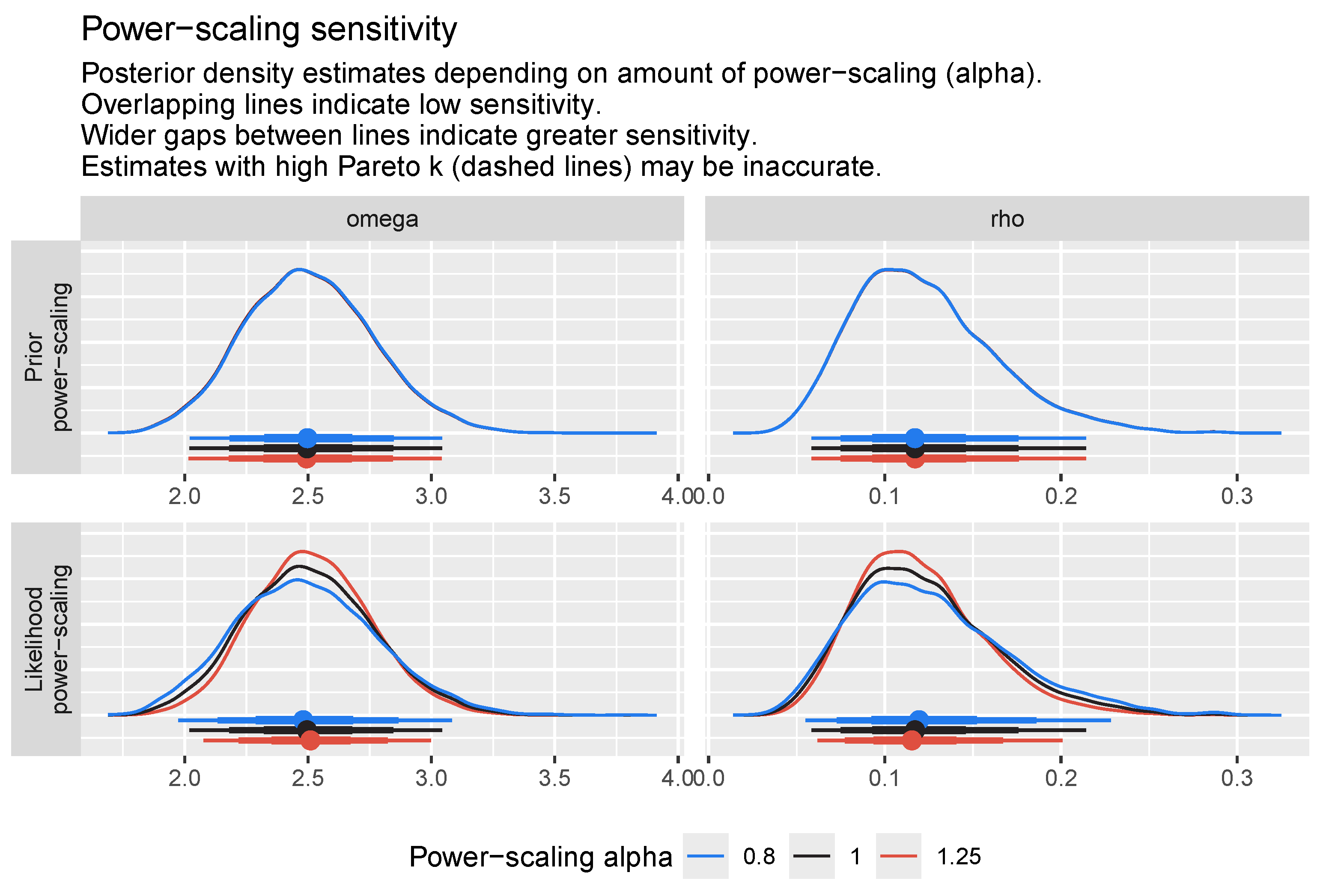
Bayesian inference offers a probabilistic approach to statistical analysis, integrating prior knowledge with observed data through Bayes’ theorem to update beliefs and make informed decisions. In this section, we present the Bayesian analysis of the dataset I using our proposed PiPLW distribution. The selection of the prior is an important step in Bayesian analysis. In this study, we have chosen weakly informative gamma distribution as priors for both unknown parameters of the PiPLW distribution, specifically $\rho \sim \mathrm{Gamma}({\alpha }_1,{\beta }_1)$ and $\omega \sim \mathrm{Gamma}({\alpha }_2,{\beta }_2)$. The hyperparameters of the priors were selected using sensitivity analysis (see Figure 11). Based on this analysis, we chose the hyperparameter values as ${\alpha }_1=0.1$, ${\beta }_1=1$, ${\alpha }_2=0.1$, and ${\beta }_2=1$.

Suppose $y_1,y_2,\dots ,y_n$ are n independent random samples drawn from the PiPLW distribution with unknown parameters $\psi =(\rho ,\omega )$. The likelihood function $\mathcal{L}\left(\mathit{y}\right|\psi )$ is expressed as follows:

$$\mathcal{L}\left(\mathit{y}\right|\psi )={\left({\displaystyle \frac{2\rho \omega log\pi }{\pi -1}}\right)}^n\prod _i^n{\pi }^{\left({\displaystyle \frac{1-e^{-\rho y_i^{\omega }}}{1+e^{-\rho y_i^{\omega }}}}\right)}{\displaystyle \frac{y^{\omega -1}{e}^{-\rho y_i^{\omega }}}{{\left(1+e^{-\rho y_i^{\omega }}\right)}^2}}$$

(13)

The joint distribution of $\mathit{y}$ and $\psi =(\rho ,\omega )$ is obtained as the product of the likelihood and prior distributions, expressed as follows:

$$\begin{array}{cc}\hfill g\left(\mathit{y}\right|\psi )=& \left\{{\left({\displaystyle \frac{2\rho \omega log\pi }{\pi -1}}\right)}^n\prod _i^n{\pi }^{\left({\displaystyle \frac{1-e^{-\rho y_i^{\omega }}}{1+e^{-\rho y_i^{\omega }}}}\right)}{\displaystyle \frac{y_i^{\omega -1}{e}^{-\rho y_i^{\omega }}}{{\left(1+e^{-\rho y_i^{\omega }}\right)}^2}}\right\}\left\{{\displaystyle \frac{{\beta }_1^{{\alpha }_1}}{\mathsf{\Gamma }\left({\alpha }_1\right)}}{\rho }^{{\alpha }_1-1}{e}^{-{\beta }_1\rho }\right\}\hfill \end{array}$$

(14)

$$\begin{array}{cc}\hfill & \left\{{\displaystyle \frac{{\beta }_2^{{\alpha }_2}}{\mathsf{\Gamma }\left({\alpha }_2\right)}}{\omega }^{{\alpha }_2-1}{e}^{-{\beta }_2\omega }\right\}\hfill \end{array}$$

(15)

The joint posterior distribution is given by the following expression:

$$\begin{array}{cc}\hfill g\left(\mathit{y}\right|\psi )\propto {\left({\displaystyle \frac{2log\pi }{\pi -1}}\right)}^n& {\rho }^{(n+{\alpha }_1-1)}{\omega }^{(n+{\alpha }_2-1)}{\displaystyle \frac{{\beta }_1^{{\alpha }_1}}{\mathsf{\Gamma }\left({\alpha }_1\right)}}{\displaystyle \frac{{\beta }_2^{{\alpha }_2}}{\mathsf{\Gamma }\left({\alpha }_2\right)}}\hfill \\ & \prod _{i=1}^n{\pi }^{\left({\displaystyle \frac{1-e^{-\rho y_i^{\omega }}}{1+e^{-\rho y_i^{\omega }}}}\right)}{\displaystyle \frac{y_i^{\omega -1}{e}^{-\rho y_i^{\omega }}}{{\left(1+e^{-\rho y_i^{\omega }}\right)}^2}}·{\rho }^{{\alpha }_1-1}{e}^{-{\beta }_1\rho }·{\omega }^{{\alpha }_2-1}{e}^{-{\beta }_2\omega }\hfill \end{array}$$

(16)

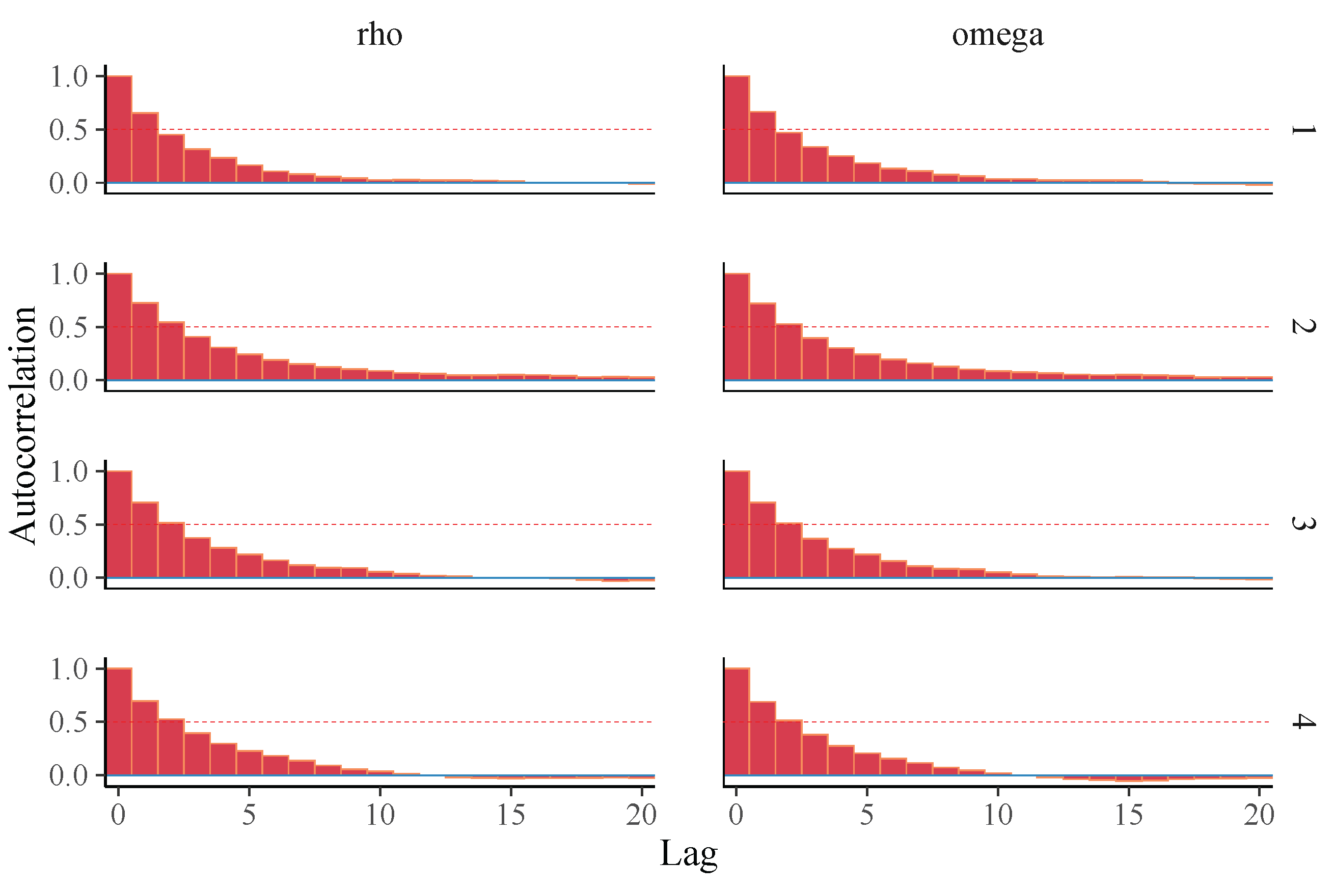
To estimate the parameter, we drew samples from the posterior distribution using the Markov Chain Monte Carlo (MCMC) method. Three widely used MCMC techniques are Gibbs Sampling, Metropolis–Hastings, and Hamiltonian Monte Carlo (HMC). Among these, HMC is particularly advantageous due to its efficiency in exploring high-dimensional parameter spaces [30]. Therefore, we utilized HMC to generate posterior samples and estimate the parameters. HMC was implemented in the rstan package in R [22]. To achieve this, we ran four Markov chains, each with 10,000 iterations, using Stan. The first 50% of the samples were designated as warm-up iterations to ensure proper convergence and adaptation of the sampler. To assess convergence, we examine trace plots, the autocorrelation function (ACF) plot, and the Gelman–Rubin statistic ($\widehat{R}$). Smooth trace plots and rapidly decaying ACF indicate good mixing and low autocorrelation, while $\widehat{R}\approx 1$ suggests proper convergence. For robust inference, the effective sample size ($n_{\mathrm{eff}}$) should exceed 10% of the total sample size. The model fit is evaluated using the Posterior Predictive Check (PPC) plot, which ensures that the simulated posterior predictions align well with the observed data. In addition, a test statistic-based p-value in PPC was used to assess model fit. P-values closer to 0.5 indicate good fit of the model, indicating that the test statistics look similar to the observed and simulated data.

7.2.1. Bayesian Parameter Estimation for Dataset I

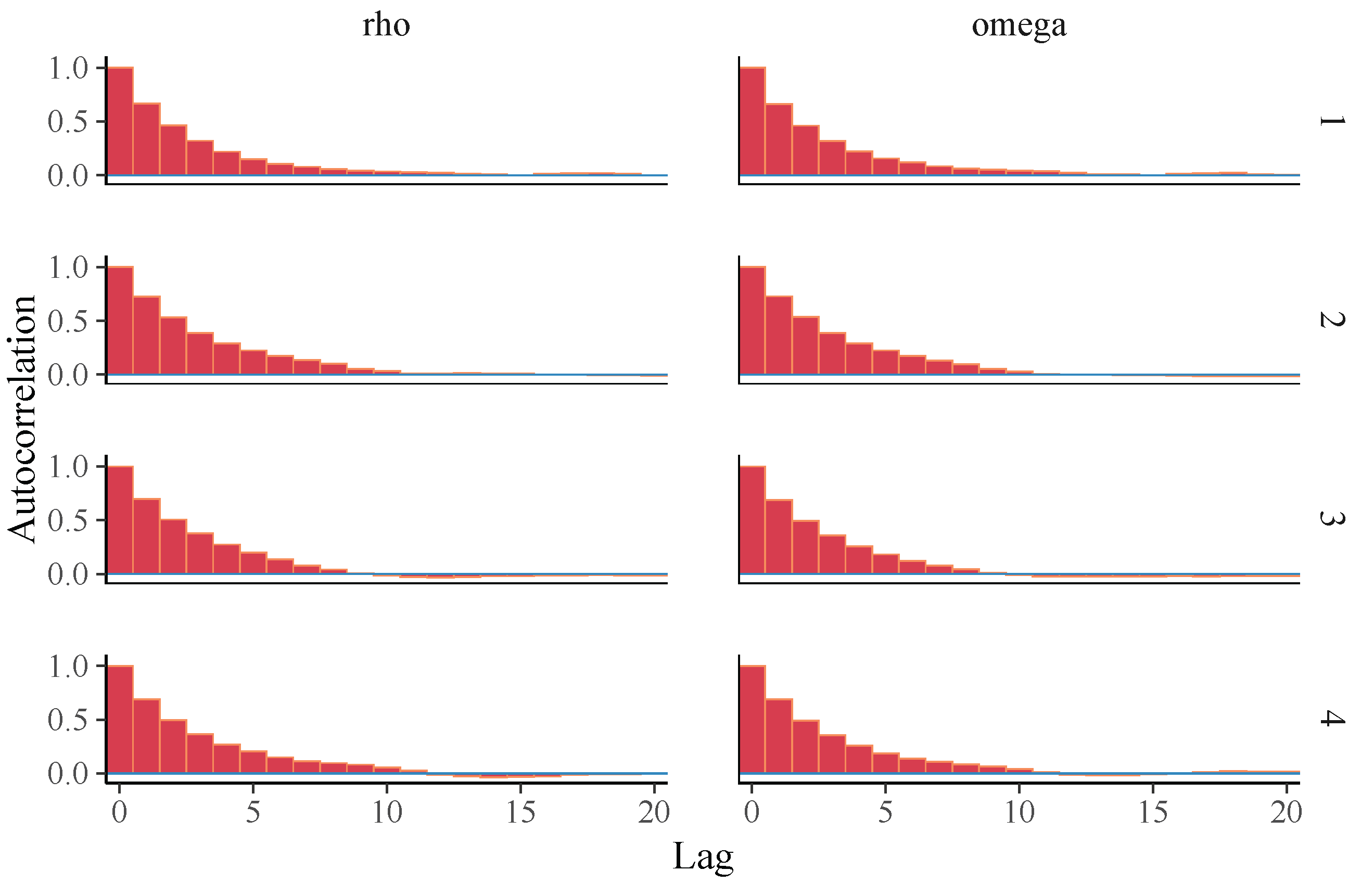
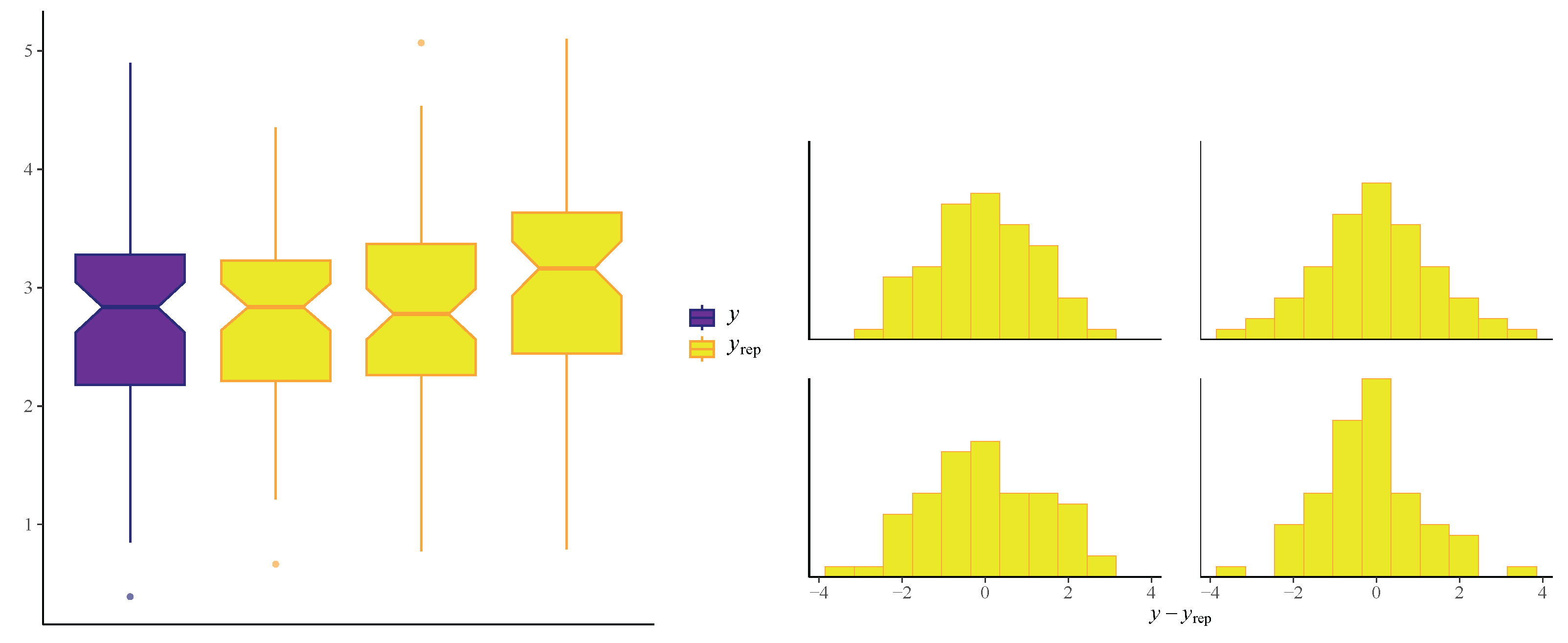
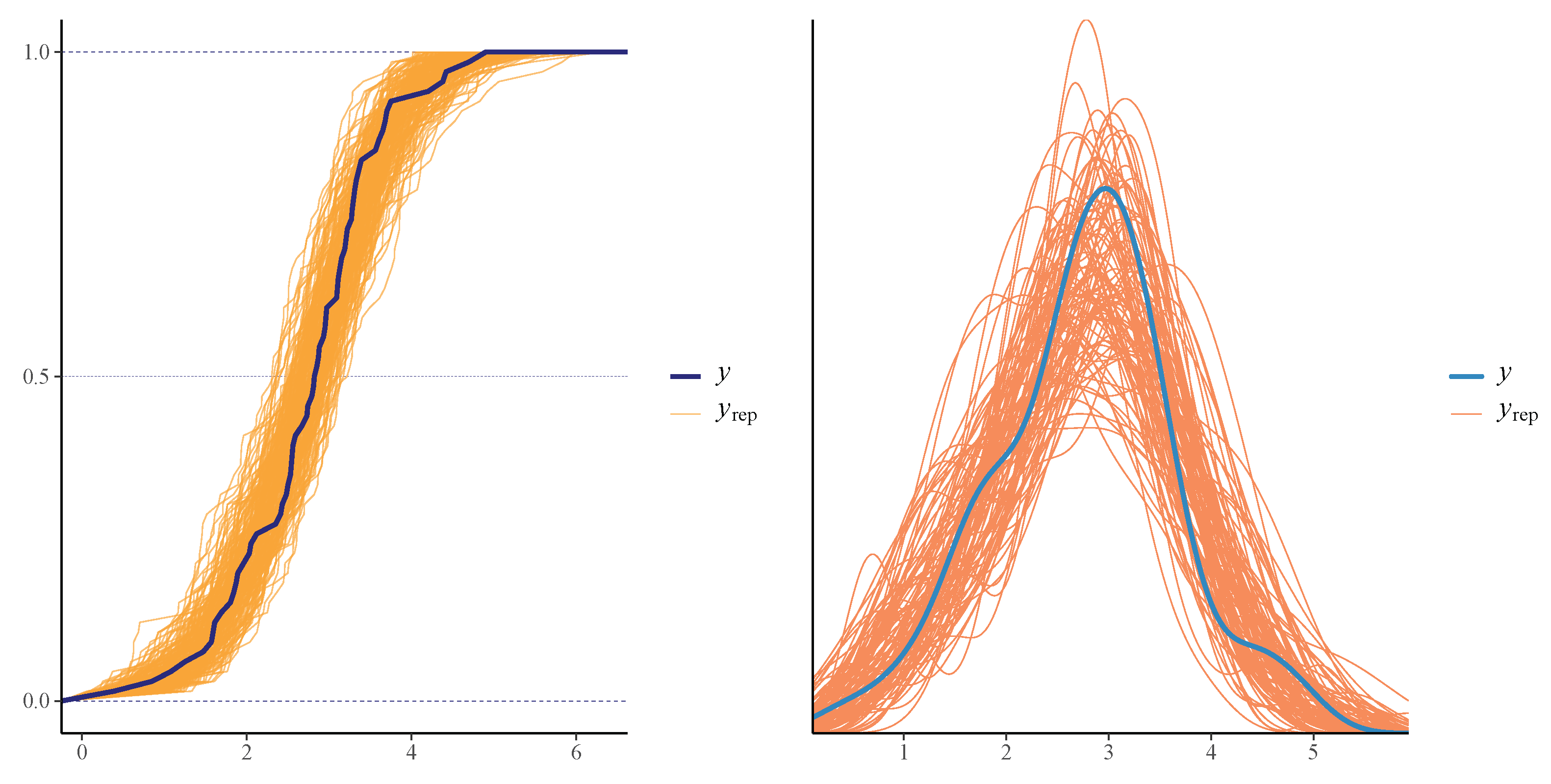
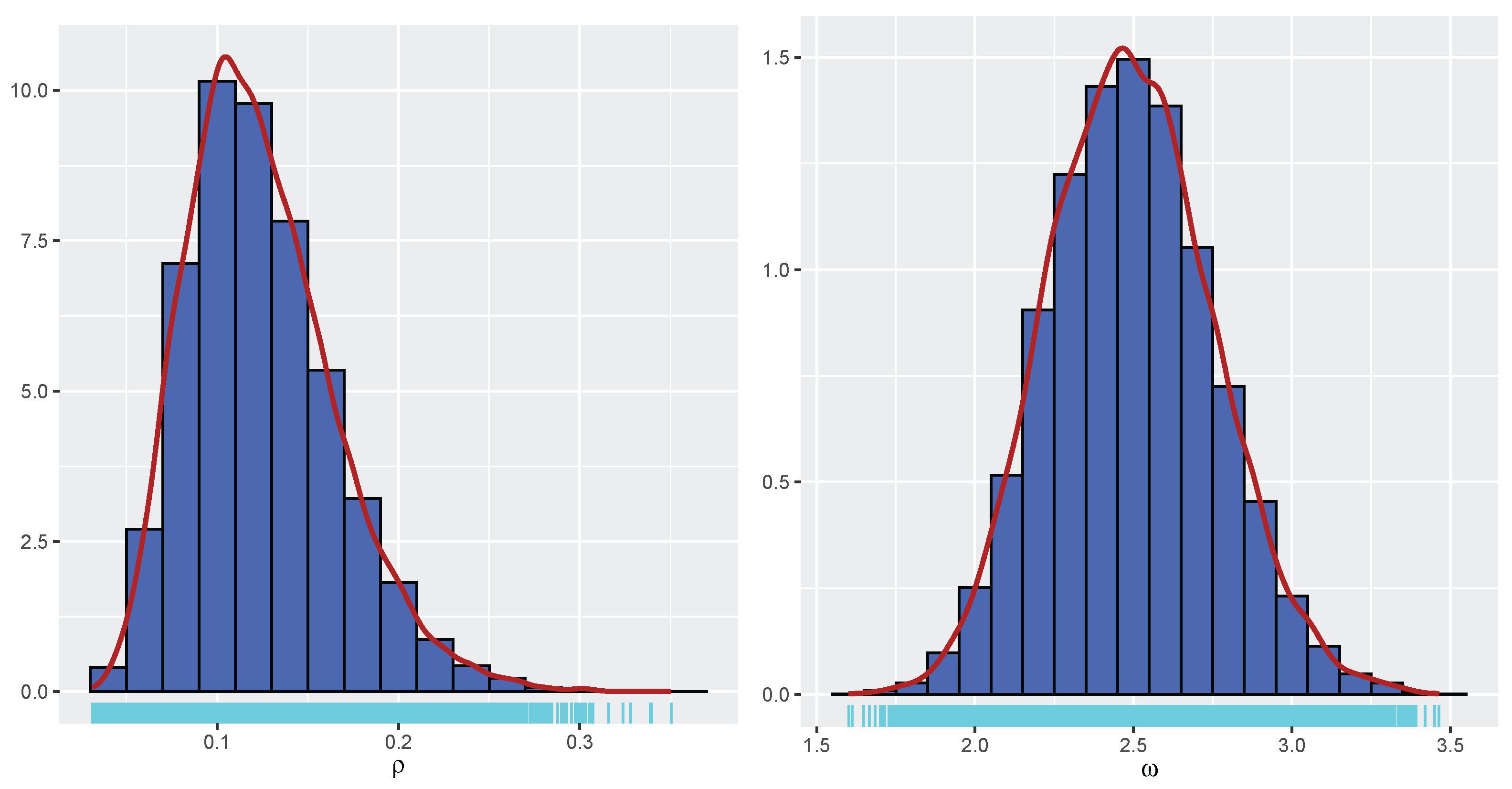
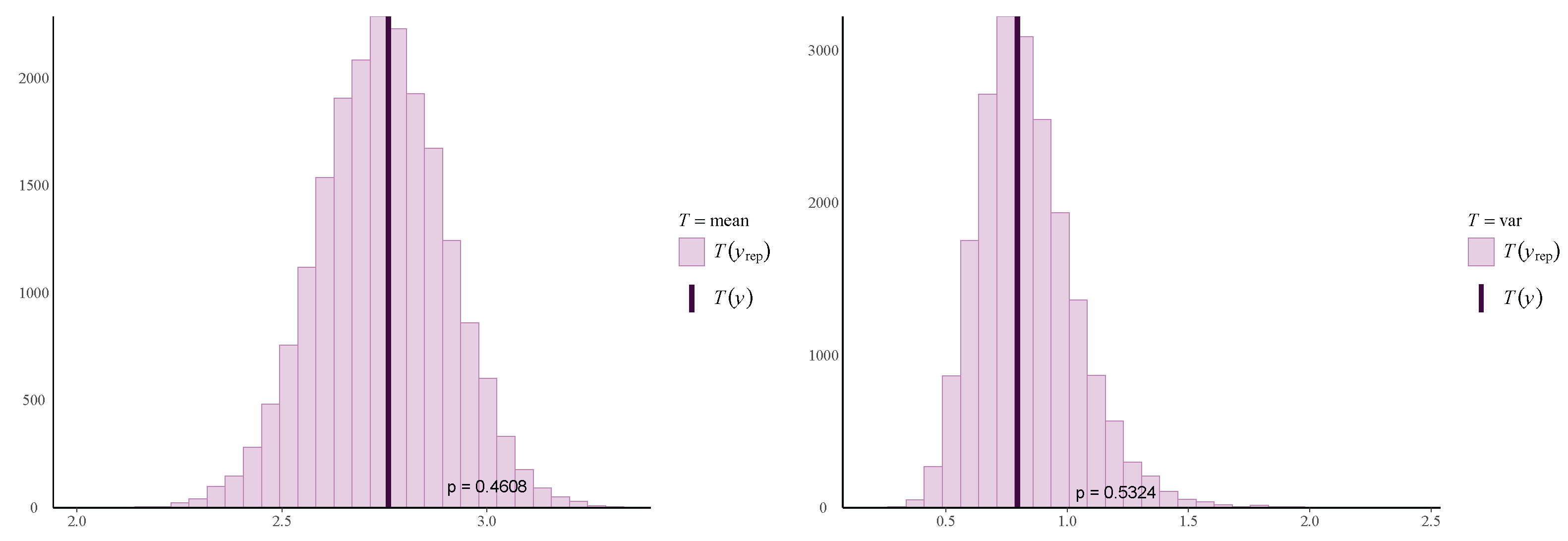
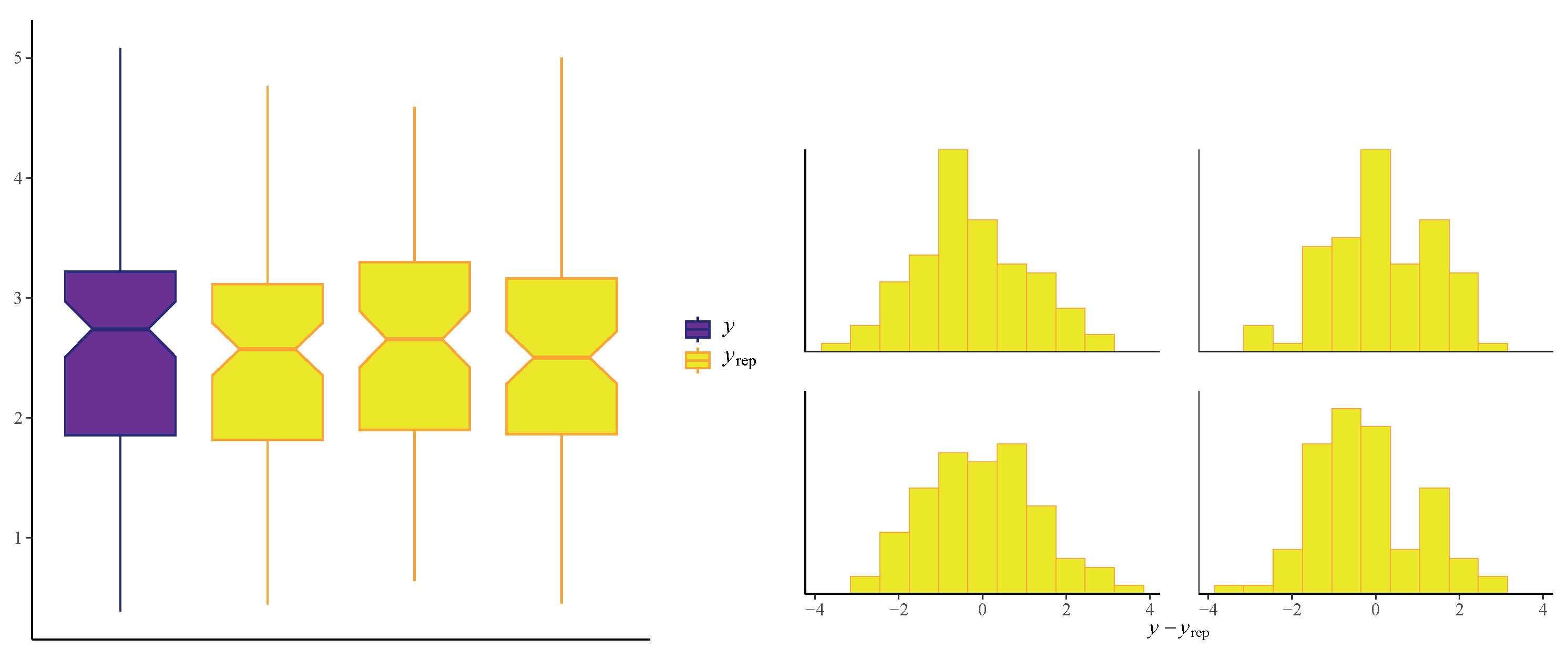
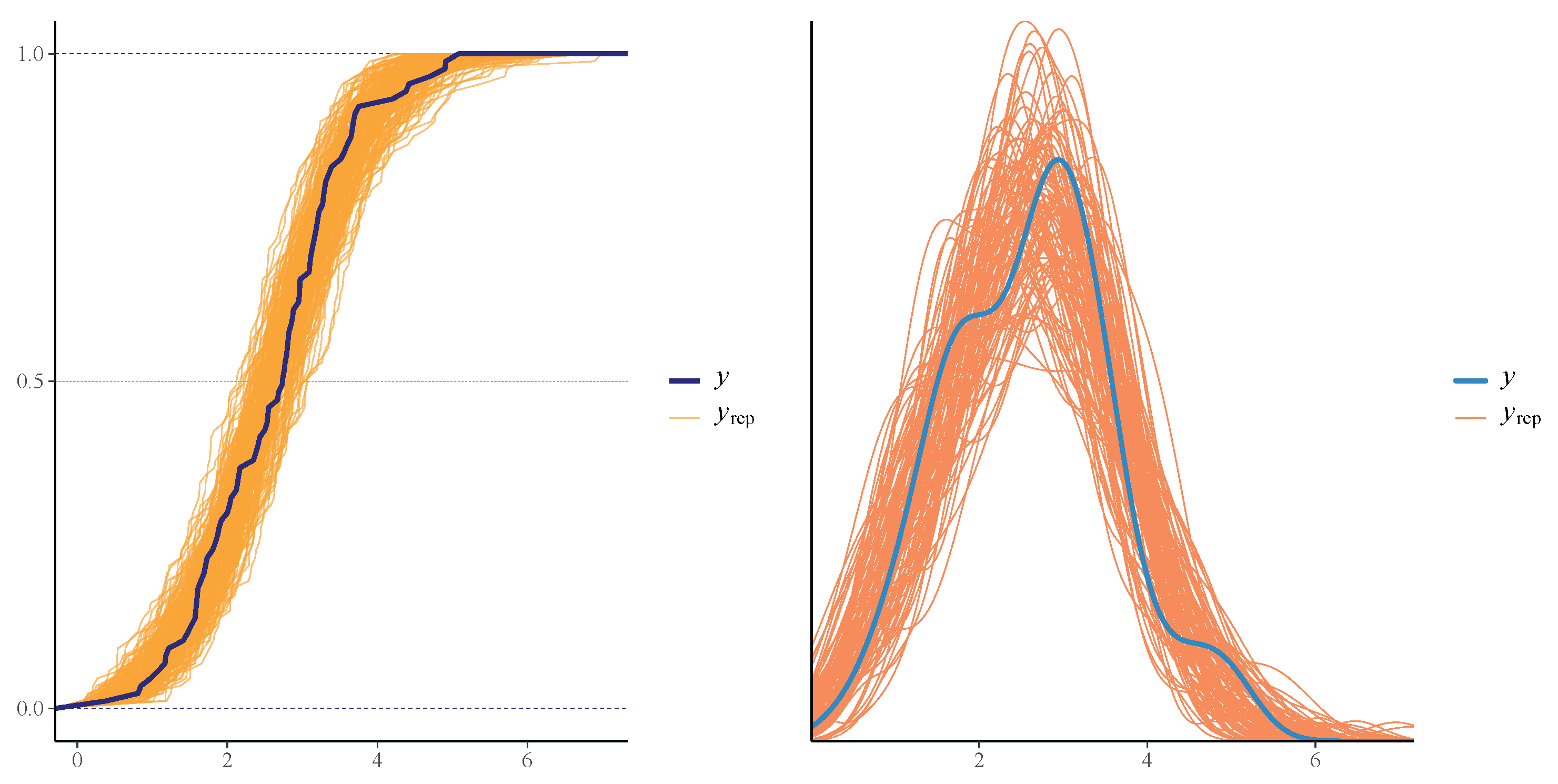
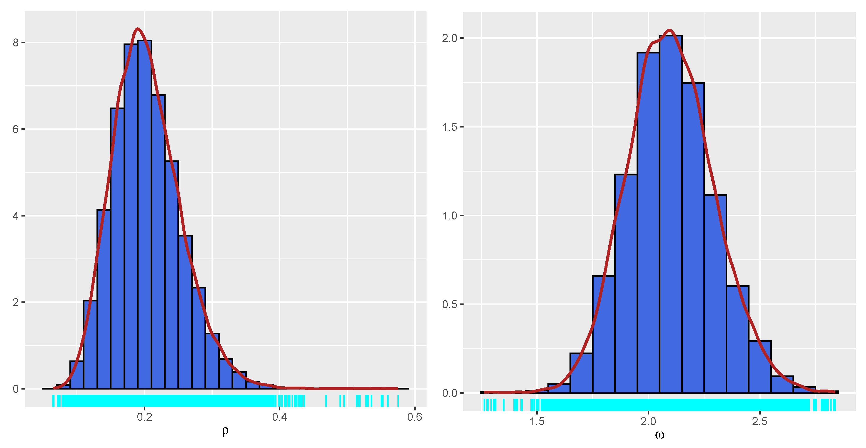
Before estimating the parameters, convergence diagnostics and model fit assessments were conducted. The trace plot in Figure 12 demonstrates that the chains mix well. The ACF plot in Figure 13 shows rapid convergence of the MCMC chains. The diagnostic results indicate that there are no signs of sample divergence (see

Table 14. Summary statistics for MCMC chains.

Chain	Accept_stat	Stepsize	Energy	Treedepth	n_leapfrog	Divergent
All chains	0.9897	0.0807	89.8796	3.5633	21.9273	0.0000
chain1	0.9874	0.0924	89.8012	3.4078	19.2660	0.0000
chain2	0.9904	0.0770	89.8849	3.5598	21.3688	0.0000
chain3	0.9866	0.0939	89.9915	3.3882	18.7660	0.0000
chain4	0.9946	0.0594	89.8407	3.8976	28.3084	0.0000

). The effective sample size exceeds 10% of the total sample size, and all $\widehat{R}$ values are close to 1 (see

Table 15. Bayesian parameter estimates with posterior summaries of dataset I.

Par	Mean	Se_mean	Sd	Median	CI	HPD	n_eff	$\widehat{\mathit{R}}$
$\rho$	0.1244	0.0007	0.0408	0.1192	[0.0597, 0.2182]	[0.0526, 0.2050]	3400	1.0012
$\omega$	2.4912	0.0044	0.2593	2.4842	[2.0096, 3.0254]	[1.9787, 2.9834]	3452	1.0010
lp__	−88.8884	0.0159	0.9997	−88.5898	[−91.6218, −87.9073]	[−90.8992, −87.8825]	3950	1.0018

). The PPC box plot and the PPC error histogram are shown in Figure 14, and the PPC ECDF and PPC density plot in Figure 15 confirm that the posterior predictions align well with the observed data, indicating a good fit of the model. Figure 16 shows well-behaved, unimodal posterior distributions for both parameters, indicating stable and reliable Bayesian estimates. In addition, the posterior predictive p-values for the mean (0.4608) and variance (0.5324) suggest a good model fit (see Figure 17). A summary of the parameter estimation is presented in Table 15.

7.2.2. Bayesian Parameter Estimation for Dataset II

Convergence diagnostics and model fit assessments were carried out for dataset II, following the same approach used for dataset I, prior to parameter estimation. Figure 18 presents the trace plots, indicating satisfactory mixing of the Markov chains. The autocorrelation plots in Figure 19 further support this by demonstrating rapid decay, suggesting efficient exploration of the posterior distribution. Additionally, the effective sample sizes exceed 10% of the total number of iterations, and all potential scale reduction factors ($\widehat{R}$) are close to 1, as summarized in

Table 16. Bayesian parameter estimates with posterior summaries.

Par	Mean	Se_mean	Sd	Median	CI	HPD	${\mathit{n}}_{\mathbf{eff}}$	$\widehat{\mathit{R}}$
$\rho$	0.2035	0.0009	0.0509	0.1989	[0.1173, 0.3136]	[0.1080, 0.3021]	3134.7960	1.0008
$\omega$	2.1006	0.0035	0.1945	2.0947	[1.7349, 2.4962]	[1.7247, 2.4840]	3159.808	1.0009
lp__	−125.0840	0.0172	1.0403	−124.7623	[−127.7768, −124.0993]	[−127.0711, −124.0746]	3647.656	1.0015

, indicating good convergence across all parameters. Furthermore, no indications of divergent transitions were observed during sampling (see

Table 17. Sampler diagnostics summary for all chains and individual chains of dataset II.

Chain	Accept_stat	Stepsize	Treedepth	N_leapfrog	Divergent	Energy
All chains	0.993	0.074	3.747	24.466	0.000	126.091
Chain 1	0.990	0.096	3.449	19.166	0.000	126.117
Chain 2	0.994	0.070	3.780	25.262	0.000	126.058
Chain 3	0.993	0.075	3.723	23.243	0.000	126.090
Chain 4	0.996	0.057	4.036	30.192	0.000	126.100

). The posterior predictive checks, including the box plot and error histogram presented in Figure 20, as well as the empirical CDF (ECDF) and density plots shown in Figure 21, demonstrate close agreement between the posterior predictions and the observed data, indicating a good model fit. Figure 22 shows well-behaved, unimodal posterior distributions for both parameters, indicating stable and reliable Bayesian estimates. In addition, the posterior predictive p-values for the mean (0.4801) and variance (0.5242) suggest a good model fit (see Figure 23). The summary of the parameter estimation is presented in Table 16.

8. Conclusions

This study introduces a novel and flexible distribution family, the $\pi$-power logistic-G family, with a particular focus on the Weibull baseline distribution, resulting in the PiPLW distribution. The proposed distribution exhibits a variety of hazard rate shapes, such as increasing, bathtub, J-shaped, and reverse J-shaped, making it suitable for a broad range of applications, particularly in reliability and survival analysis.

We explored the statistical properties of the PiPLW distribution and employed the MLE method for parameter estimation. A Monte Carlo simulation study demonstrated that the MLE performs well, with mean square errors decreasing as sample sizes increase, even for small samples. The distribution’s utility was further demonstrated by applying it to two real-world datasets from reliability engineering. Goodness-of-fit statistics and model selection criteria confirmed the superior performance of the PiPLW distribution compared to seven competing models. Additionally, a Bayesian approach using Hamiltonian Monte Carlo (HMC) via the ‘rstan’ package in R was successfully applied, showing the model’s compatibility with both frequentist and Bayesian frameworks. Under the Bayesian framework, the proposed model exhibited excellent predictive performance for both datasets, further underscoring its potential for diverse applications. For practitioners in reliability engineering and survival analysis, this study provides a salient choice for modeling data across diverse domains, delivering robust and efficient parameter estimation compared to several existing alternatives.

Despite the promising results, several limitations must be acknowledged. First, the model’s performance was assessed using only two datasets from the reliability domain, which may limit generalizability. Second, the proposed distribution assumes complete data without censoring; extending the methodology to handle censored or truncated data would enhance its applicability in medical and actuarial studies. The current simulation study focuses on moderate-to-large sample sizes and does not explicitly evaluate performance under small sample sizes or high censoring levels.

Future research can explore several directions. The $\pi$-power logistic-G family can be extended using other baseline distributions to create new flexible models tailored to specific data types. Furthermore, the PiPLW distribution can be incorporated into regression models to handle covariates and extended to multivariate settings to address complex data structures. Finally, real-world applications in areas such as biomedical research, finance, and environmental studies should be pursued to validate the model’s utility further.

References

1. Alzaatreh, A.; Lee, C.; Famoye, F. A New Method for Generating Families of Continuous Distributions. METRON 2013, 71, 63–79. [Google Scholar] [CrossRef]
2. Ahmad, Z.; Mahmoudi, E.; Dey, S. A new family of heavy tailed distributions with an application to the heavy tailed insurance loss data. Commun. Stat. Simul. Comput. 2022, 51, 4372–4395. [Google Scholar] [CrossRef]
3. Lone, M.A.; Jan, T.R. A New Pi-Exponentiated Method for Constructing Distributions with an Application to Weibull Distribution. Reliab. Theory Appl. 2023, 18, 94–109. [Google Scholar]
4. Kumar, P.; Sapkota, L.P.; Kumar, V. π-Power Half Logistic-G Family: Applications to Medical and Traffic Data. Reliab. Theory Appl. 2023, 4, 575–590. [Google Scholar]
5. Nassar, M.; Alzaatreh, A.; Abo-Kasem, O.; Mead, M.; Mansoor, M. A New Family of Generalized Distributions Based on Alpha Power Transformation with Application to Cancer Data. Ann. Data Sci. 2018, 5, 421–436. [Google Scholar] [CrossRef]
6. Mead, M.E.; Cordeiro, G.M.; Afify, A.Z.; Al Mofleh, H. The Alpha Power Transformation Family: Properties and Applications. Pak. J. Stat. Oper. Res. 2019, 15, 525–545. [Google Scholar] [CrossRef]
7. Mahdavi, A.; Kundu, D. A New Method for Generating Distributions with an Application to Exponential Distribution. Commun. Stat. Theory Methods 2017, 46, 6543–6557. [Google Scholar] [CrossRef]
8. Alghamdi, A.S.; ALoufi, S.F.; Baharith, L.A. The Sine Alpha Power-G Family of Distributions: Characterizations, Regression Modeling, and Applications. Symmetry 2025, 17, 468. [Google Scholar] [CrossRef]
9. Kawo, K.N.; Goshu, A.T.; Kindo, B.P. A New Alpha Power Transformation of Logistic Distribution with Its Properties and Applications. J. Probab. Stat. 2025, 2025, 9594412. [Google Scholar] [CrossRef]
10. Maruthan, S.K.; Venkatachalam, N. Alpha Power Transformation of Lomax Distribution: Properties and Applications. Thail. Stat. 2022, 20, 669–685. [Google Scholar]
11. Ihtisham, S.; Khalil, A.; Manzoor, S.; Khan, S.A.; Ali, A. Alpha-Power Pareto Distribution: Its Properties and Applications. PLoS ONE 2019, 14, e0218027. [Google Scholar] [CrossRef]
12. Hozaien, H.E.; Dayian, G.R.A.; El-Helbawy, A.A. Modeling Extreme Values with Alpha Power Inverse Pareto Distribution. Meas. Sci. Rev. 2023, 23, 55–62. [Google Scholar] [CrossRef]
13. Hozaien, H.E.; Dayian, G.R.A.L.; El-Helbawy, A.A. Kumaraswamy Distribution Based on Alpha Power Transformation Methods. Asian J. Probab. Stat. 2021, 11, 14–29. [Google Scholar] [CrossRef]
14. Benkhelifa, L. Alpha power Topp-Leone Weibull distribution: Properties, characterizations, regression modeling and applications. J. Stat. Manag. Syst. 2022, 25, 1945–1970. [Google Scholar] [CrossRef]
15. Gomaa, R.S.; Hebeshy, E.A.; El Genidy, M.M.; El-Desouky, B.S. Alpha-Power of the Power Ailamujia Distribution: Properties and Applications. J. Stat. Appl. Probab. 2023, 12, 701–723. [Google Scholar] [CrossRef]
16. Klakattawi, H.S.; Aljuhani, W.H. A New Technique for Generating Distributions Based on a Combination of Two Techniques: Alpha Power Transformation and Exponentiated TX Distributions Family. Symmetry 2021, 13, 412. [Google Scholar] [CrossRef]
17. Alotaibi, R.; Okasha, H.; Rezk, H.; Nassar, M. A New Weighted Version of Alpha Power Transformation Method: Properties and Applications to COVID-19 and Software Reliability Data. Phys. Scr. 2021, 96, 125221. [Google Scholar] [CrossRef]
18. Elbatal, I.; Ahmad, Z.; Elgarhy, M.; Almarashi, A.M. A New Alpha Power Transformed Family of Distributions: Properties and Applications to the Weibull Model. J. Nonlinear Sci. Appl. 2018, 12, 1–20. [Google Scholar] [CrossRef]
19. McCool, J.I. Using the Weibull Distribution: Reliability, Modeling, and Inference; Wiley: Hoboken, NJ, USA, 2012. [Google Scholar]
20. Sapkota, L.P. Exponentiated–Exponential Logistic Distribution: Some Properties and Application. Janapriya J. Interdiscip. Stud. 2020, 9, 100–108. [Google Scholar] [CrossRef]
21. Henningsen, A.; Toomet, O. maxLik: A Package for Maximum Likelihood Estimation in R. Comput. Stat. 2011, 26, 443–458. [Google Scholar] [CrossRef]
22. R Core Team. R: A Language and Environment for Statistical Computing; R Foundation for Statistical Computing: Vienna, Austria, 2024; Available online: https://www.R-project.org/ (accessed on 14 August 2025).
23. Oguntunde, P.E.; Balogun, O.S.; Okagbue, H.I.; Bishop, S.A. The Weibull-Exponential Distribution: Its Properties and Applications. J. Appl. Sci. 2015, 15, 1305–1311. [Google Scholar] [CrossRef]
24. Sapkota, L.P.; Kumar, V. Half Cauchy Generalized Rayleigh Distribution: Theory and Application. South East Asian J. Math. Math. Sci. 2023, 19, 1–15. [Google Scholar] [CrossRef]
25. Nichols, M.D.; Padgett, W.J. A Bootstrap Control Chart for Weibull Percentiles. Qual. Reliab. Eng. Int. 2006, 22, 141–151. [Google Scholar] [CrossRef]
26. Kelter, R. Statistical Rethinking: A Bayesian Course with Examples in R and STAN; Taylor & Francis: Abingdon, UK, 2020. [Google Scholar]
27. Gauthami, P.; Mariyamma, K.D.; Kavya, P. A Modified Inverse Weibull Distribution Using KM Transformation. Reliab. Theory Appl. 2023, 18, 35–42. [Google Scholar]
28. Cordeiro, G.M.; Afify, A.Z.; Yousof, H.M.; Cakmakyapan, S.; Ozel, G. The Lindley Weibull Distribution: Properties and Applications. An. Acad. Bras. Cienc. 2018, 90, 2579–2598. [Google Scholar] [CrossRef] [PubMed]
29. Nassar, M.; Dey, S.; Kumar, D. Logarithm Transformed Lomax Distribution with Applications. Calcutta Stat. Assoc. Bull. 2018, 70, 122–135. [Google Scholar] [CrossRef]
30. Neal, R.M. MCMC Using Hamiltonian Dynamics. In Handbook of Markov Chain Monte Carlo; Brooks, S., Gelman, A., Jones, G., Meng, X.-L., Eds.; Chapman & Hall/CRC: Boca Raton, FL, USA, 2011; pp. 113–162. [Google Scholar]
Figure 1. Some shapes of the PDF and HRF of PiPLW distribution.
Axioms 14 00643 g001
Figure 2. Behavior of skewness and kurtosis.
Axioms 14 00643 g002
Figure 3. Total Time on Test (TTT) plots for the real datasets I and II.
Axioms 14 00643 g003
Figure 4. Graphs of KM estimate of PiPLW distribution for datasets I and II.
Axioms 14 00643 g004
Figure 5. Plot of profile log-likelihood for dataset I.
Axioms 14 00643 g005
Figure 6. Plot of profile log-likelihood for dataset II.
Axioms 14 00643 g006
Figure 7. Graphs of fitted PDF and CDF for dataset I.
Axioms 14 00643 g007
Figure 8. Graphs of fitted PDF and CDF for dataset II.
Axioms 14 00643 g008
Figure 9. P-P plots for dataset I.
Axioms 14 00643 g009
Figure 10. P-P plots for dataset II.
Axioms 14 00643 g010
Figure 11. Plots for power scaling sensitivity for ρ G a m m a ( 0.1 , 1 ) and ω G a m m a ( 0.1 , 1 ) .
Axioms 14 00643 g011
Figure 12. Trace plots.
Axioms 14 00643 g012
Figure 13. Autocorrelation plots for different chains.
Axioms 14 00643 g013
Figure 14. Box plots of observed data y and posterior prediction y r e p and histogram of predicted errors.
Axioms 14 00643 g014
Figure 15. Fitted CDF of the posterior distribution (left) and density of observed and simulated data (right).
Axioms 14 00643 g015
Figure 16. Histograms of posterior distribution.
Axioms 14 00643 g016
Figure 17. Posterior predictive p-value plots based on test statistics for the mean (left) and variance (right); vertical lines denote observed values.
Axioms 14 00643 g017
Figure 18. Trace plots of dataset II.
Axioms 14 00643 g018
Figure 19. Autocorrelation plots for different chains for dataset II.
Axioms 14 00643 g019
Figure 20. Box plots of observed data y and posterior prediction y r e p and histogram of predicted errors for dataset II.
Axioms 14 00643 g020
Figure 21. Fitted CDF of the posterior distribution (left) and density of observed and simulated data (right) for dataset II.
Axioms 14 00643 g021
Figure 22. Histograms of posterior distribution for dataset II.
Axioms 14 00643 g022
Figure 23. Posterior predictive p-value plots based on test statistics for the mean (left) and variance (right) for dataset II; vertical lines denote observed values.
Axioms 14 00643 g023