
Dynamic Analysis of an Amensalism Model Driven by Multiple Factors: The Interwoven Impacts of Refuge, the Fear Effect, and the Allee Effect


Abstract
1. Introduction
2. Construction of the Mathematical Model
2.1. Model Assumptions
- 1.
- Refuge and fear effect for the first species.
- 2.
- The Allee effect for the second species.
- 3.
- Amensalism relationship.
- 4.
- Parameter constraints.
- 5.
- Simplifying assumptions.
2.2. Model Formulation
3. Global Dynamics of System (5)
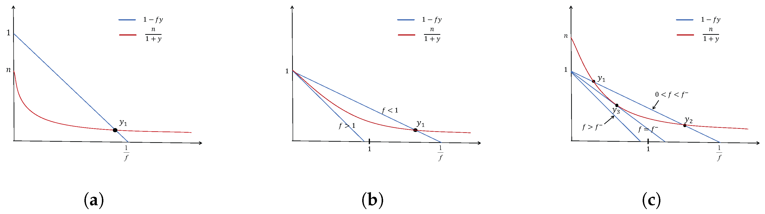
3.1. Existence of Equilibria
- (1)
- When , has one positive root ;
- (2)
- When and , has one positive root ;
- (3)
- When
- (i)
- and , has two positive roots, and ;
- (ii)
- and , has one positive, root .
- (1)
- For (weak Allee effect);
- (a)
- (b)
- (2)
- For ,
- (a)
- when
- (i)
- (ii)
- (b)
- (3)
- For (strong Allee effect),
- (a)
- when
- (i)
- (ii)
- (iii)
- (b)
- when ,
- (i)
- (ii)
- (c)
- (1)
- When , then if , and if .
- (2)
- When and , if , and if .
- (3)
- When
- (a)
- and , if , if , and if ;
- (b)
- and , if , and if .
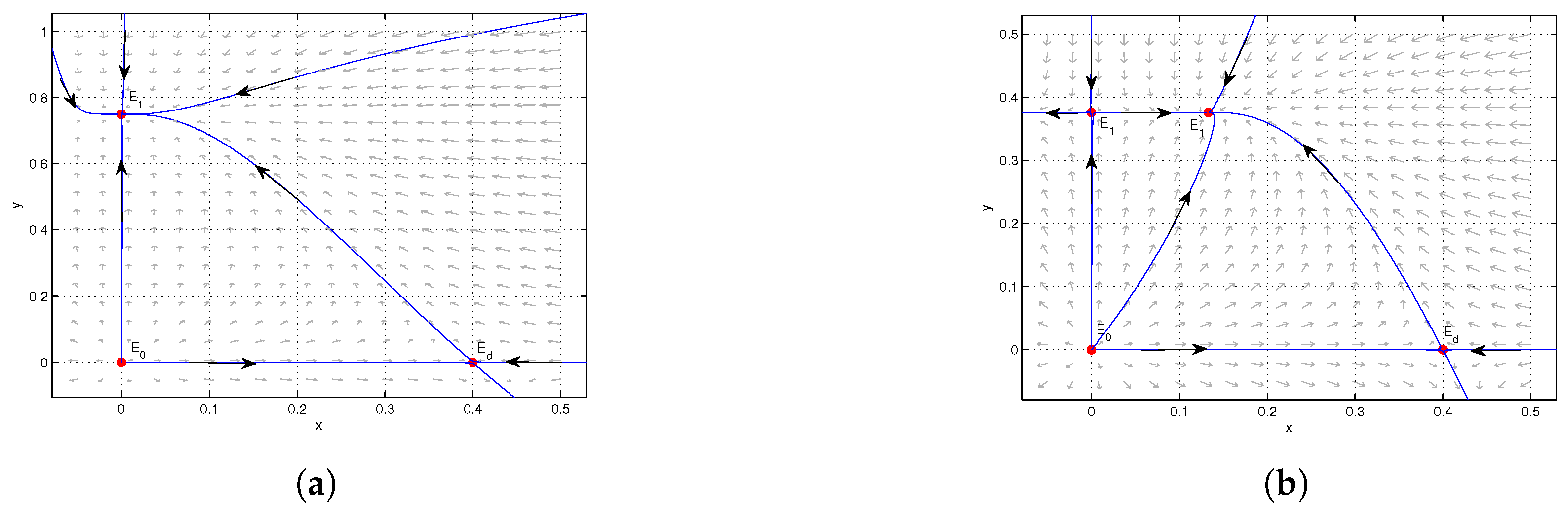
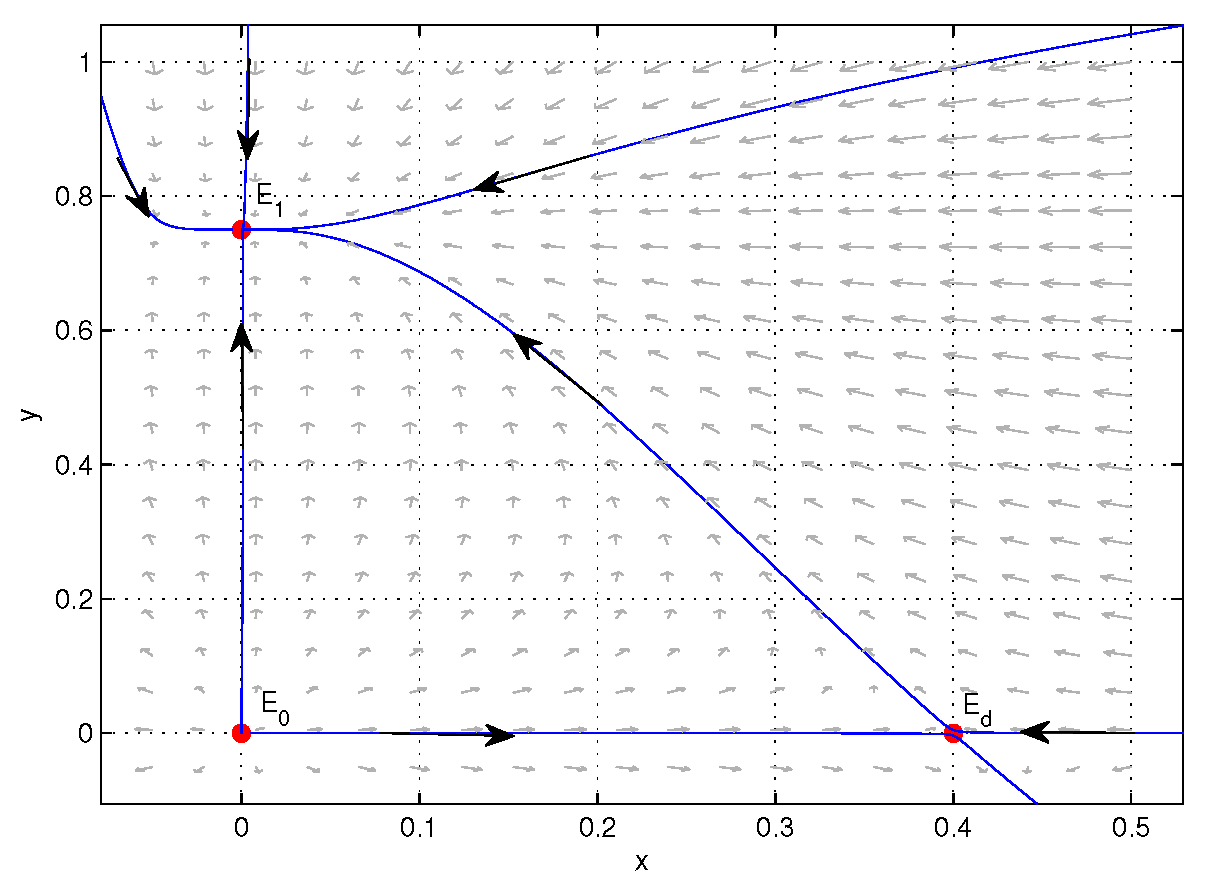
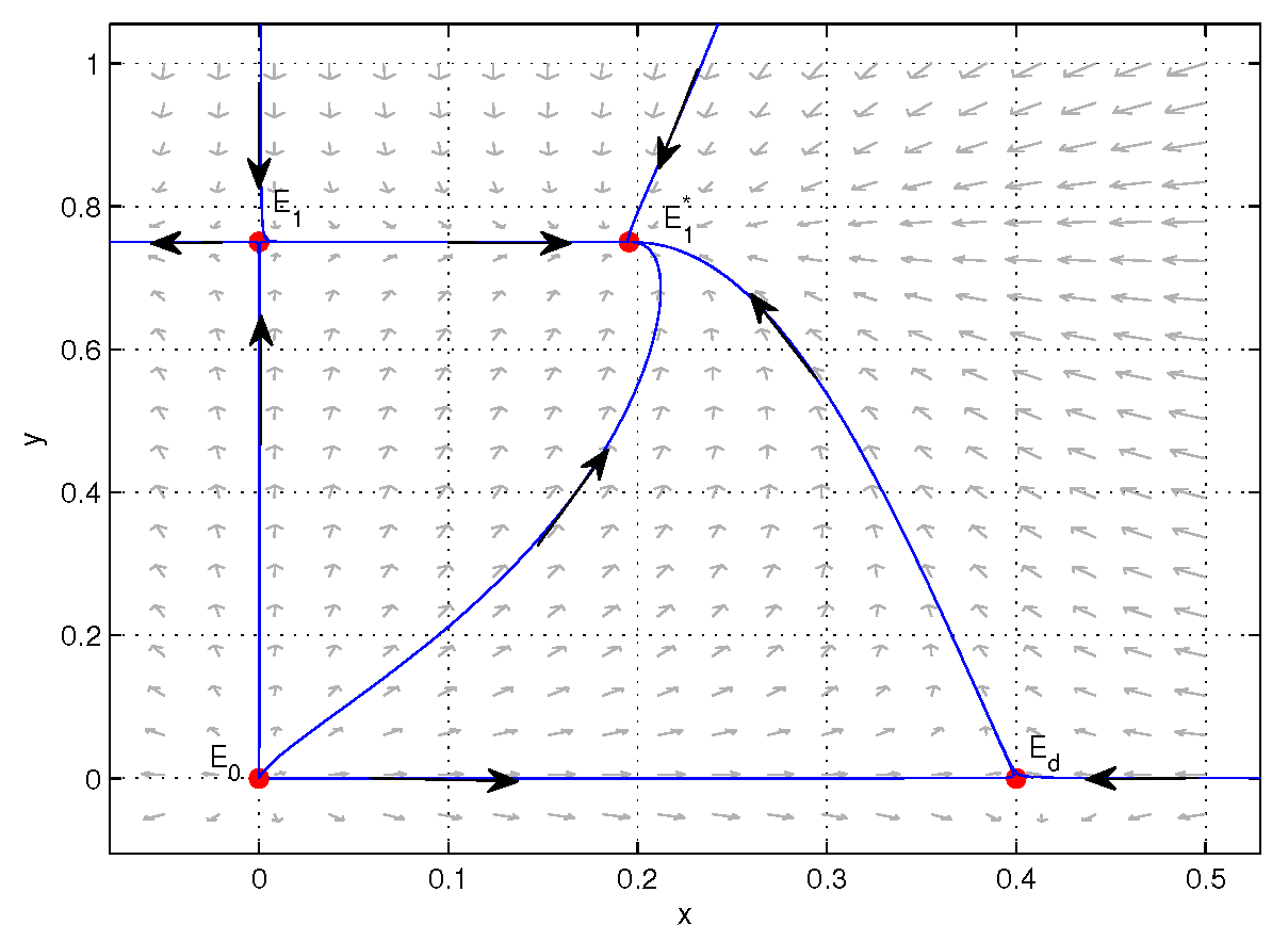
3.2. Stability of Equilibria
- (1)
- When , is an unstable node and is a saddle.
- (2)
- When , is a saddle and is a stable node.
- (3)
- When ,
- (i)
- , is a repelling saddle-node, and is an attracting saddle-node;
- (ii)
- , is a saddle of codimension 2, and is an unstable node.
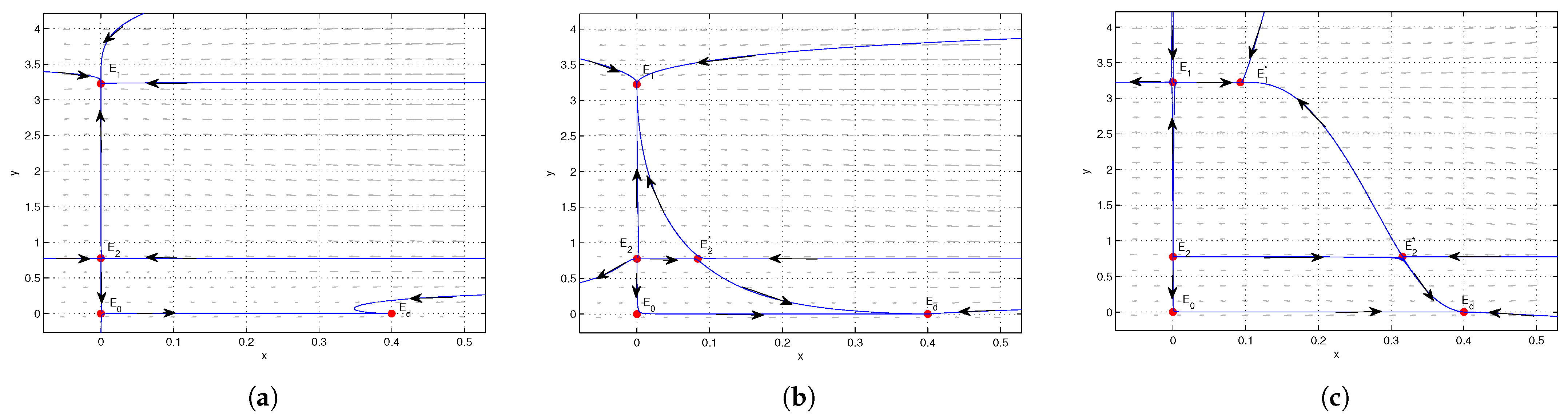
- (1)
- For , when exists (i.e., or and or and ),
- (i)
- and , is a saddle;
- (ii)
- and , is a stable node;
- (iii)
- and , is an attracting saddle-node.
- (2)
- For , when exists (i.e., and ),
- (i)
- and , is an unstable node;
- (ii)
- and , is a saddle;
- (iii)
- and , is a repelling saddle-node.
- (3)
- For , when exists (i.e., and ),
- (i)
- and , is a repelling saddle-node;
- (ii)
- and , is an attracting saddle-node;
- (iii)
- and , is a saddle.
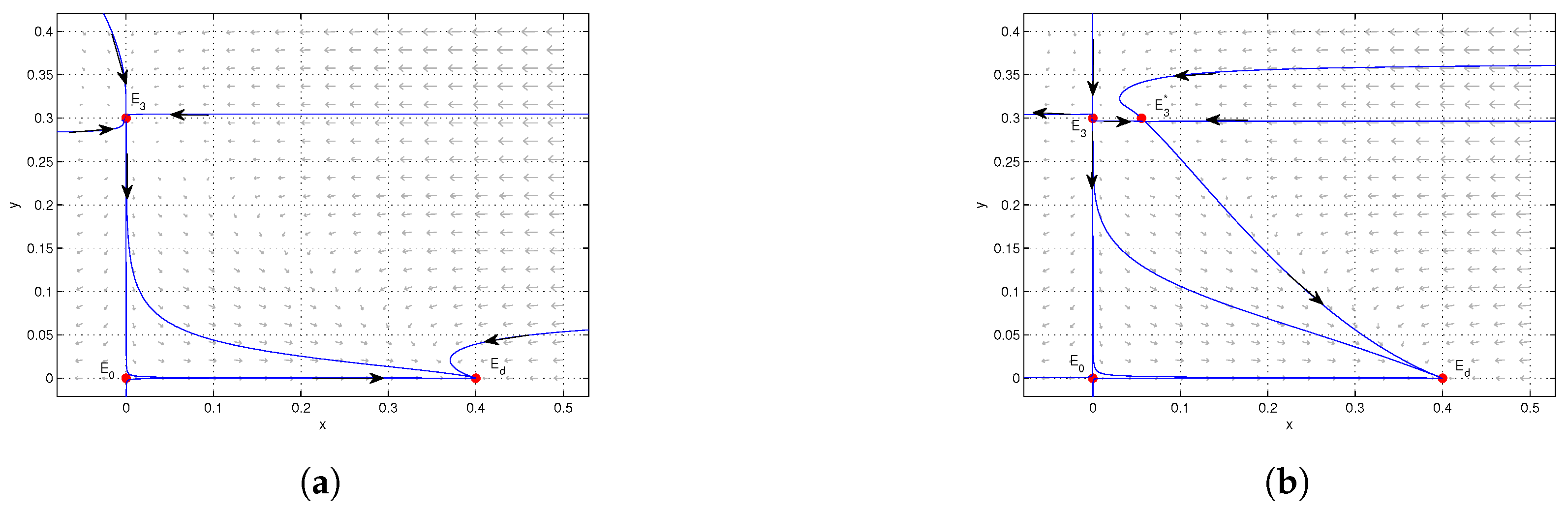
- (1)
- For , when exists, is a stable node.
- (2)
- For , when exists, is a saddle.
- (3)
- For , when exists, is an attracting saddle-node.
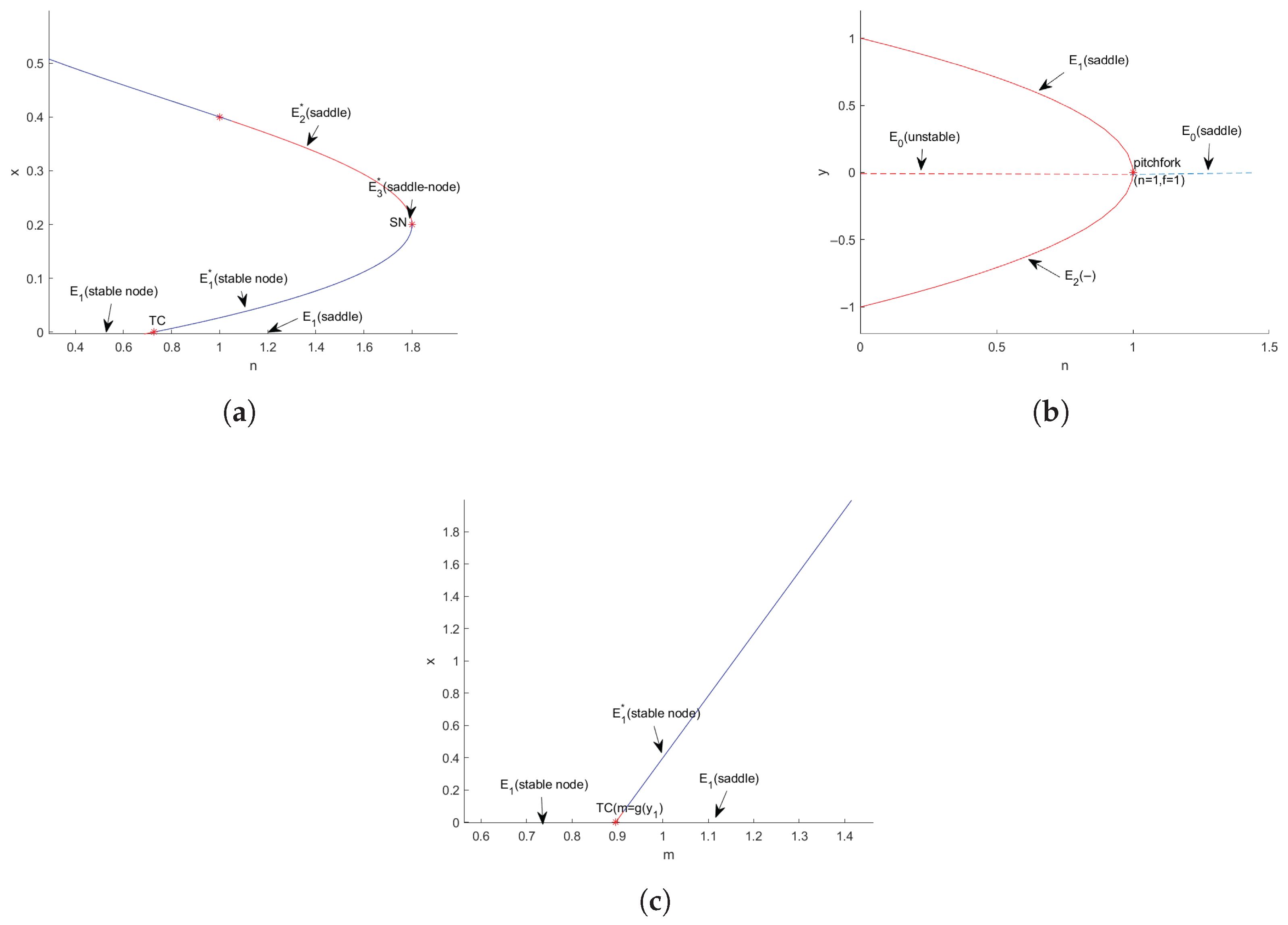
3.3. Bifurcation Analysis
3.3.1. Transcritical Bifurcation
3.3.2. Pitchfork Bifurcation
3.3.3. Saddle-Node Bifurcation
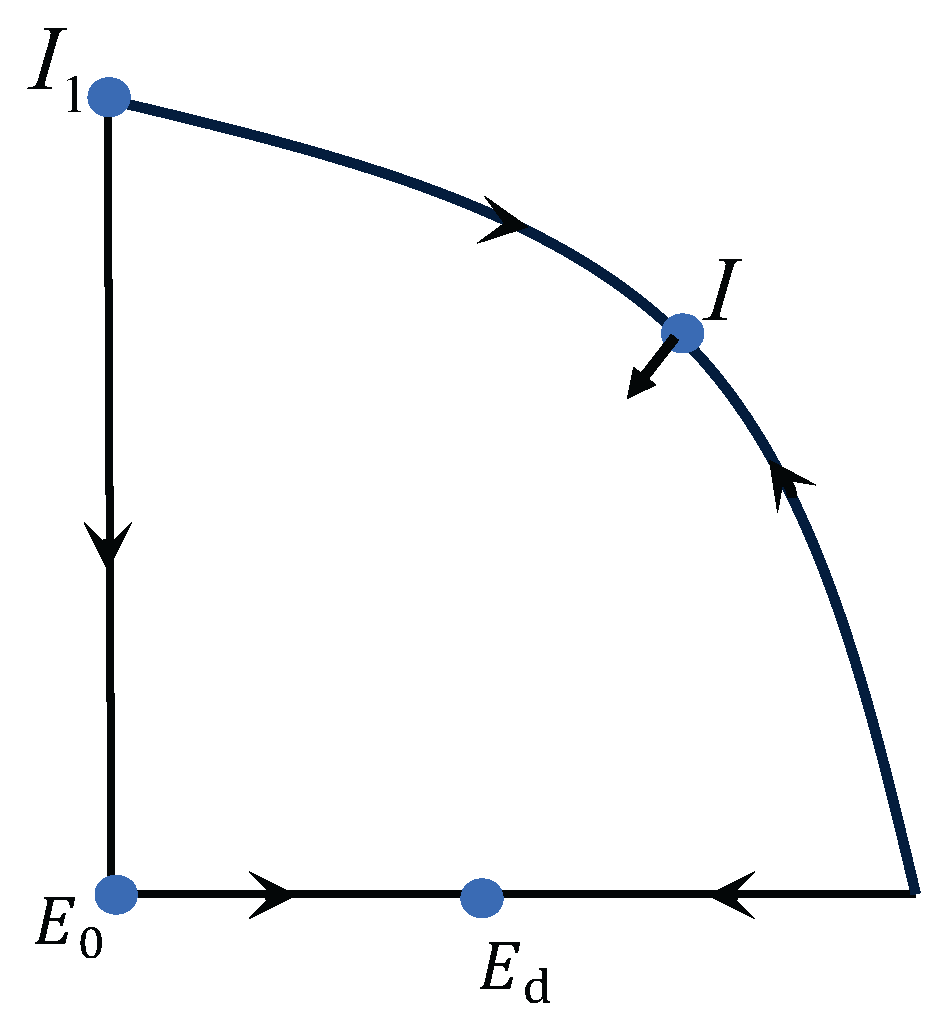
3.4. Global Structure
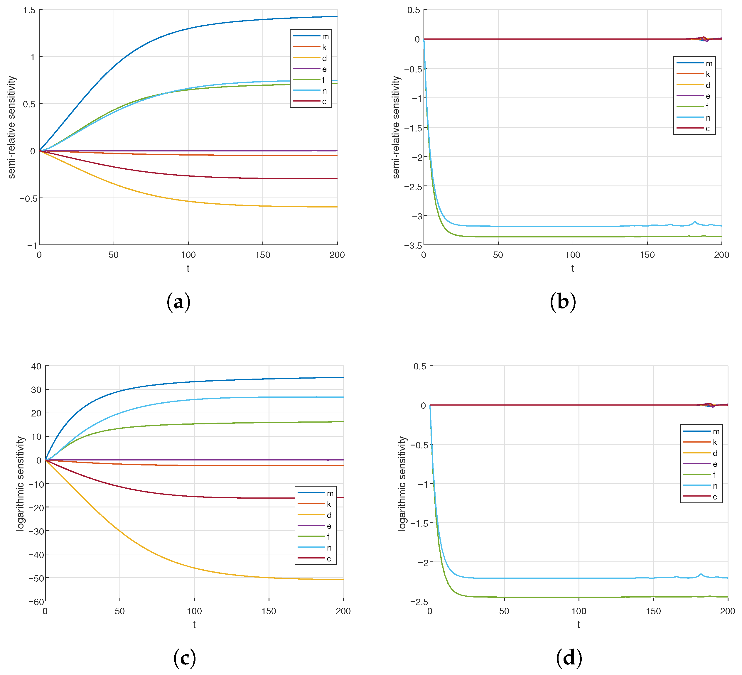
3.5. Sensitivity Analysis
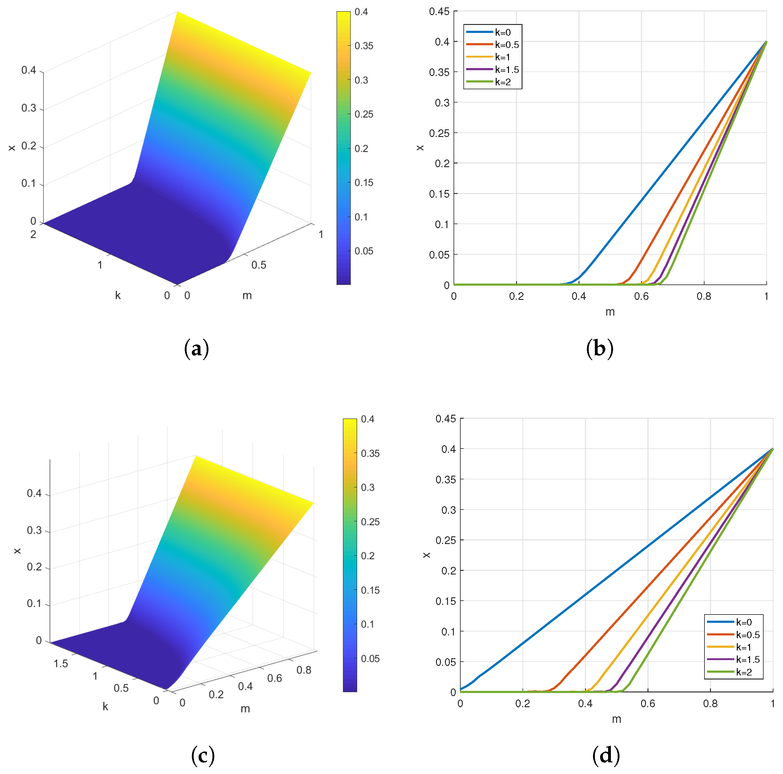
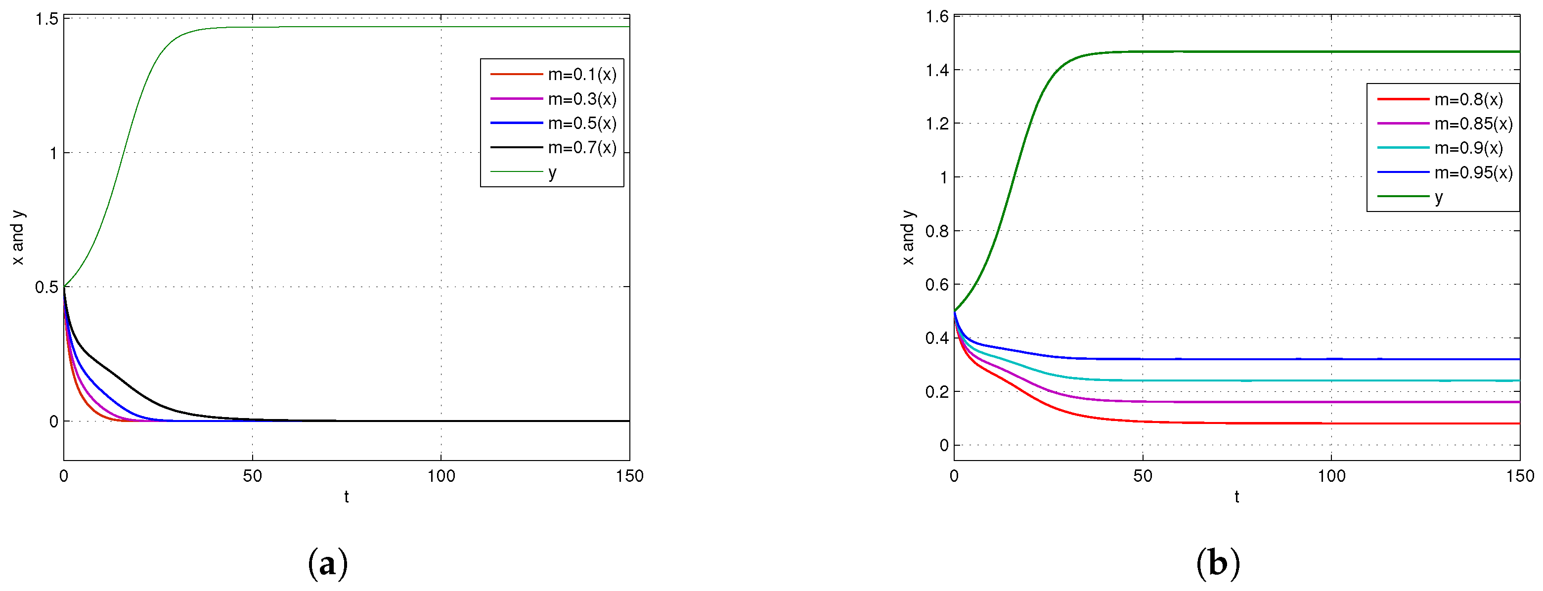
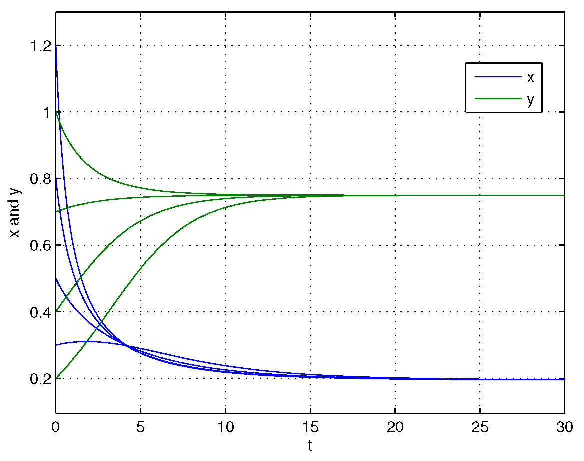
4. Numerical Simulations
5. Conclusions
Author Contributions
Funding
Data Availability Statement
Conflicts of Interest
References
- Veiga, J.P. Commensalism, amensalism, and synnecrosis. In Encyclopedia of Evolutionary Biology; Academic Press: Cambridge, MA, USA, 2016; Volume 2, pp. 322–328. [Google Scholar]
- Xi, X.; Griffin, J.N.; Sun, S. Grasshoppers amensalistically suppress caterpillar performance and enhance plant biomass in an alpine meadow. Oikos 2013, 122, 1049–1057. [Google Scholar] [CrossRef]
- Ogada, D.L.; Gadd, M.E.; Ostfeld, R.S. Impacts of large herbivorous mammals on bird diversity and abundance in an African savanna. Oecologia 2018, 156, 387–397. [Google Scholar] [CrossRef] [PubMed]
- Hughes, L. The effects of climate change on plant-pollinator interactions. Ecol. Lett. 2000, 3, 73–82. [Google Scholar]
- Veiga, J.P.; Wamiti, W.; Polo, V.; Muchai, M. Interphyletic relationships in the use of nesting cavities: Mutualism, competition and amensalism among hymenopterans and vertebrates. Naturwissenschaften 2013, 100, 827–834. [Google Scholar] [CrossRef] [PubMed]
- Sun, G. Qualitative analysis on two populations amensalism model. J. Jiamusi Univ. 2003, 21, 283–286. [Google Scholar]
- Liu, Y.; Zhao, L.; Huang, X. Stability and bifurcation analysis of two species amensalism model with Michaelis-Menten type harvesting and a cover for the first species. Adv. Differ. Equ. 2018, 2018, 295. [Google Scholar] [CrossRef]
- Zhao, M.; Ma, Y.; Du, Y. Global dynamics of an amensalism system with Michaelis-Menten type harvesting. Electron. Res. Arch. 2023, 31, 549–574. [Google Scholar] [CrossRef]
- Guan, X.; Chen, F. Dynamical analysis of a two species amensalism model with Beddington–DeAngelis functional response and Allee effect on the second species. Nonlinear Anal. Real World Appl. 2019, 48, 71–93. [Google Scholar] [CrossRef]
- Zhu, Q.; Chen, F.; Li, Z.; Chen, L. Global dynamics of two-species amensalism model with Beddington–DeAngelis functional response and fear effect. Int. J. Bifurc. Chaos 2024, 34, 245007. [Google Scholar] [CrossRef]
- Luo, D.; Wang, Q. Global dynamics of a Holling-II amensalism system with nonlinear growth rate and Allee effect on the first species. Int. J. Bifurc. Chaos 2021, 31, 2150050. [Google Scholar] [CrossRef]
- Luo, D.; Wang, Q. Global dynamics of a Beddington–DeAngelis amensalism system with weak Allee effect on the first species. Appl. Math. Comput. 2021, 408, 126368. [Google Scholar] [CrossRef]
- Chen, B. Dynamic behaviors of a non-selective harvesting Lotka–Volterra amensalism model incorporating partial closure for the populations. Adv. Differ. Equ. 2018, 2018, 111. [Google Scholar] [CrossRef]
- Xie, X.; Chen, F.; He, M. Dynamic behaviors of two species amensalism model with a cover for the first species. J. Math. Comput. Sci. 2016, 16, 395–401. [Google Scholar] [CrossRef]
- Liu, H.; Yu, H.; Dai, C.; Ma, Z.; Wang, Q.; Zhao, M. Dynamical analysis of an aquatic amensalism model with non-selective harvesting and Allee effect. Math. Biosci. Eng. 2021, 18, 8857–8882. [Google Scholar] [CrossRef] [PubMed]
- Lei, C. Dynamic behaviors of a stage structure amensalism system with a cover for the first species. Adv. Differ. Equ. 2018, 2018, 272. [Google Scholar] [CrossRef]
- Wei, Z.; Xia, Y.; Zhang, T. Stability and bifurcation analysis of an amensalism model with weak Allee effect. Qual. Theory Dyn. Syst. 2020, 19, 23. [Google Scholar] [CrossRef]
- Wu, R. A two species amensalism model with non-monotonic functional response. Commun. Math. Biol. Neurosci. 2016, 2016, 19. [Google Scholar]
- Wu, R.; Li, L.; Lin, Q. A Holling type commensal symbiosis model involving Allee effect. Commun. Math. Biol. Neurosci. 2018, 2018, 6. [Google Scholar] [CrossRef]
- Zhao, M.; Du, Y. Stability and bifurcation analysis of an amensalism system with Allee effect. Adv. Differ. Equ. 2020, 2020, 341. [Google Scholar] [CrossRef]
- Alhadi, A.R.S.A.; Naji, R.K. The contribution of amensalism and parasitism in the three-species ecological system’s dynamic. Commun. Math. Biol. Neurosci. 2024, 2024, 33–45. [Google Scholar]
- Singh, M.K. Dynamical study and optimal harvesting of a two-species amensalism model incorporating nonlinear harvesting. Appl. Appl. Math. 2023, 18, 19. [Google Scholar]
- Peckarsky, B.L.; Abrams, P.A.; Bolnick, D.I.; Dill, L.M.; Grabowski, J.H.; Luttbeg, B.; Orrock, J.L.; Peacor, S.D.; Preisser, E.L.; Schmitz, O.J.; et al. Revisiting the classics: Considering nonconsumptive effects in textbook examples of predator–prey interactions. Ecology 2008, 89, 2416–2425. [Google Scholar] [CrossRef] [PubMed]
- Polis, G.A.; Myers, C.A.; Holt, R.D. The ecology and evolution of intraguild predation: Potential competitors that eat each other. Annu. Rev. Ecol. Syst. 1989, 20, 297–330. [Google Scholar] [CrossRef]
- Dong, Y.; Wu, D.; Shen, C.; Ye, L. Influence of fear effect and predator-taxis sensitivity on dynamical behavior of a predator–prey model. Z. Angew. Math. Phys. 2022, 73, 25. [Google Scholar] [CrossRef]
- Sarkar, K.; Khajanchi, S. Impact of fear effect on the growth of prey in a predator-prey interaction model. Ecol. Complex. 2020, 42, 100826. [Google Scholar] [CrossRef]
- Thirthar, A.A.; Majeed, S.J.; Alqudah, M.A.; Panja, P.; Abdeljawad, T. Fear effect in a predator-prey model with additional food, prey refuge and harvesting on super predator. Chaos Solitons Fractals 2022, 159, 112091. [Google Scholar] [CrossRef]
- Wang, J.; Cai, Y.; Fu, S.; Wang, W. The effect of the fear factor on the dynamics of a predator-prey model incorporating the prey refuge. Chaos Interdiscip. J. Nonlinear Sci. 2019, 29, 083109. [Google Scholar] [CrossRef] [PubMed]
- Zhang, H.; Cai, Y.; Fu, S.; Wang, W. Impact of the fear effect in a prey-predator model incorporating a prey refuge. Appl. Math. Comput. 2019, 356, 328–337. [Google Scholar] [CrossRef]
- Wu, R.; Zhao, L.; Lin, Q. Stability analysis of a two species amensalism model with Holling-II functional response and a cover for the first species. J. Nonlinear Funct. Anal. 2016, 2016, 46. [Google Scholar]
- Chong, Y.; Zhu, Q.; Li, Q.; Chen, F. Dynamic behaviors of a two species amensalism model with a second species dependent cover. Eng. Lett. 2024, 32, 1553–1561. [Google Scholar]
- Yang, W.; Chen, M. The impact of predator-dependent prey refuge on the dynamics of a Leslie-Gower predator-prey model. Asian Res. J. Math. 2023, 19, 203–211. [Google Scholar] [CrossRef]
- Huang, X.; Chen, F. The influence of the Allee effect on the dynamic behaviors of two species amensalism system with a refuge for the first species. Adv. Appl. Math. 2019, 8, 1166–1180. [Google Scholar] [CrossRef]
- Osakabe, M.; Hongo, K.; Funayama, K.; Osumi, S. Amensalism via webs causes unidirectional shifts of dominance in spider mite communities. Oecologia 2006, 150, 496–505. [Google Scholar] [CrossRef] [PubMed]
- Courchamp, F.; Clutton-Brock, T.; Grenfell, B. Inverse density dependence and the Allee effect. Trends Ecol. Evol. 1999, 14, 405–410. [Google Scholar] [CrossRef] [PubMed]
- Schreiber, S. Allee effects, extinctions, and chaotic transients in simple population models. Theor. Popul. Biol. 2003, 64, 201–209. [Google Scholar] [CrossRef] [PubMed]
- Guo, X.; Ding, L.; Hui, Y.; Song, X. Dynamics of an amensalism system with strong Allee effect and nonlinear growth rate in deterministic and fluctuating environment. Nonlinear Dyn. 2024, 112, 21389–21408. [Google Scholar] [CrossRef]
- Dennis, B. Allee effects: Population growth, critical density, and the chance of extinction. Nat. Resour. Model. 1989, 3, 481–538. [Google Scholar] [CrossRef]
- Zhang, Z.; Ding, T.; Huang, W.; Dong, Z. Qualitative Theory of Differential Equations; Science Press: Beijing, China, 1997. [Google Scholar]
- Polking, J.C. Ordinary Differential Equations Using MATLAB; Pearson Education: Chennai, India, 2009. [Google Scholar]
- Perko, L. Differential Equations and Dynamical Systems; Springer: New York, NY, USA, 2001. [Google Scholar]
- Wang, S.; Xie, Z.; Zhong, R.; Wu, Y. Stochastic analysis of a predator–prey model with modified Leslie–Gower and Holling type II schemes. Nonlinear Dyn. 2020, 101, 1245–1262. [Google Scholar] [CrossRef]
- Wang, S.; Wang, Z.; Xu, C.; Jiao, G. Sensitivity analysis and stationary probability distributions of a stochastic two-prey one-predator model. Appl. Math. Lett. 2021, 116, 106996. [Google Scholar] [CrossRef]
- Tripathi, J.P.; Meghwani, S.S.; Thakur, M.; Abbas, S. A modified Leslie–Gower predator-prey interaction model and parameter identifiability. Commun. Nonlinear Sci. Numer. Simul. 2018, 54, 331–346. [Google Scholar] [CrossRef]
- Quarteroni, A.; Sacco, R.; Saleri, F. Numerical Mathematics; Springer Science & Business Media: Berlin/Heidelberg, Germany, 2010. [Google Scholar]
- Dhooge, A.; Govaerts, W.; Kuznetsov, Y.A. MATCONT: A MATLAB package for numerical bifurcation analysis of ODEs. ACM Trans. Math. Softw. (TOMS) 2003, 29, 141–164. [Google Scholar] [CrossRef]


| Parameter | Symbol | Dimension | Ecological Meaning |
|---|---|---|---|
| First species density | x | Population density of the first species at time | |
| Second species density | y | Population density of the second species at time | |
| Refuge proportion | m | Dimensionless | Proportion of protected habitat reducing amensalistic interactions, |
| Fear level | k | Fear level of the first species towards the second species | |
| Birth rate | Birth and rate of the first species | ||
| Mortality rate | Mortality rate of the first species | ||
| Intraspecific competition | b | Density-dependent resource limitation within the first species | |
| Intraspecific competition | f | Density-dependent resource limitation within the second species | |
| Impact parameter | c | Strength of amensalistic effect per encounter | |
| Intrinsic growth rate | e | Maximum growth rate of the second species under ideal conditions | |
| Allee threshold | a | Additive Allee effect parameter governing the strength and shape of the effect | |
| Allee intensity | n | Additive Allee effect parameter |
| Equilibrium | Existence | Type | |
|---|---|---|---|
| Always exists | , Unstable node | ||
| , Saddle | |||
| Always exists | , Saddle | ||
| , Saddle-node | |||
| , Unstable node | |||
| , Stable node | |||
| , Saddle | |||
| , Stable node | |||
| , Saddle-node | |||
| , Unstable node | |||
| , Saddle | |||
| , Saddle-node | |||
| , Saddle-node | |||
| , Saddle | |||
| Stable node | |||
| Saddle | |||
| Saddle-node |
Disclaimer/Publisher’s Note: The statements, opinions and data contained in all publications are solely those of the individual author(s) and contributor(s) and not of MDPI and/or the editor(s). MDPI and/or the editor(s) disclaim responsibility for any injury to people or property resulting from any ideas, methods, instructions or products referred to in the content. |
© 2025 by the authors. Licensee MDPI, Basel, Switzerland. This article is an open access article distributed under the terms and conditions of the Creative Commons Attribution (CC BY) license (https://creativecommons.org/licenses/by/4.0/).
Share and Cite
Huang, Y.; Chen, F.; Chen, L.; Li, Z. Dynamic Analysis of an Amensalism Model Driven by Multiple Factors: The Interwoven Impacts of Refuge, the Fear Effect, and the Allee Effect. Axioms 2025, 14, 567. https://doi.org/10.3390/axioms14080567
Huang Y, Chen F, Chen L, Li Z. Dynamic Analysis of an Amensalism Model Driven by Multiple Factors: The Interwoven Impacts of Refuge, the Fear Effect, and the Allee Effect. Axioms. 2025; 14(8):567. https://doi.org/10.3390/axioms14080567
Chicago/Turabian StyleHuang, Yuting, Fengde Chen, Lijuan Chen, and Zhong Li. 2025. "Dynamic Analysis of an Amensalism Model Driven by Multiple Factors: The Interwoven Impacts of Refuge, the Fear Effect, and the Allee Effect" Axioms 14, no. 8: 567. https://doi.org/10.3390/axioms14080567
APA StyleHuang, Y., Chen, F., Chen, L., & Li, Z. (2025). Dynamic Analysis of an Amensalism Model Driven by Multiple Factors: The Interwoven Impacts of Refuge, the Fear Effect, and the Allee Effect. Axioms, 14(8), 567. https://doi.org/10.3390/axioms14080567