Second-Order Implicit–Explicit Difference Scheme for Pseudoparabolic Equations with Nonlinear Flux

Abstract

In this work we propose a new second-order implicit–explicit difference scheme for a pseudoparabolic equation with a nonlinear flux term. The proposed method is evaluated in comparison with two known numerical approaches. The significance of this study stems from its relevance to physical and mechanical models, including the Benjamin–Bona–Mahony (–Burgers) equations, which arise as specific instances of the considered equation. A stability analysis of the constructed scheme is conducted. Furthermore, the method is generalized to address a two-dimensional case. Several numerical experiments are carried out to assess the accuracy and efficiency of the proposed scheme.

1. Introduction

Pseudoparabolic equations describe many physical and biological phenomena, including multiphase flow in porous media [1], nonlinear dispersive wave propagation [2,3,4], unsteady channel flows [5], population aggregation and recovery [6], solvent uptake in polymers [7], heat conduction [8,9], etc. They are also used to analyze non-stationary processes in semiconductors with sources [2,3,10].

Various analytical and numerical approaches have been developed for solving pseudoparabolic equations, particularly in the linear case. The existence, uniqueness, regularity, and asymptotic behavior of solutions were discussed in [11]. The authors in [12] established the well-posedness of solutions and examined the qualitative properties of solutions related to turbulent heat or mass transfer. The well-posedness of two distinct pseudoparabolic models describing the same electrical conduction phenomenon in heterogeneous media was analyzed in [13].

In the classical work of [4], the following long-wave model was derived:

$${\displaystyle \frac{\partial v}{\partial t}}-\nu {\displaystyle \frac{\partial v}{\partial x}}={\displaystyle \frac{{\partial }^{2}v}{\partial x^2}}+\epsilon {\displaystyle \frac{{\partial }^{3}v}{\partial t\partial x^2}},$$

(1)

where $v(x,t)$ represents the horizontal fluid velocity, ${\displaystyle \frac{{\partial }^{2}v}{\partial x^2}(x,t)}$ is the dispersive term, and ${\displaystyle \frac{{\partial }^{3}v}{\partial t\partial x^2}(x,t)}$ is the dissipative term. For $\epsilon =0$, Equation (1) reduces to the well-known Burgers equation [3,14].

Considering Equation (1) with the classical boundary conditions

$$v(0,t)=v(1,t)=0,$$

(2)

an a priori estimate is readily obtained:

$$\mathbb{E}\left(t\right)\le \mathbb{E}\left(0\right)e^{-ct},c=\mathrm{const}.>0,\mathbb{E}\left(t\right)={∥{\displaystyle \frac{\partial v}{\partial x}}∥}_2^2+{∥v∥}_2^2.$$

(3)

By the Sobolev embedding theorem, it follows that the solution $v(x,t)$ remains bounded for all $t\in [0,+\infty )$.

In [15], systems of hyperbolic and pseudo-parabolic type PDEs were studied. Well-posedness was illustrated and a numerical method, based on spectral approximation in space using Legendre polynomials, was constructed. A Crank–Nicolson scheme for linear pseudoparabolic equations with variable coefficients was analyzed in [9]. The authors of [16] studied the stability of an implicit finite difference scheme for problems with nonlocal integral conditions. An alternating-direction implicit method for the 2D version of such problems was constructed in [17], while operator splitting was applied in [18] to model incompressible two-phase flow in porous media. In [19,20], a fast convolution-based artificial boundary condition was used to develop a finite difference scheme for a linear pseudoparabolic equation.

Nonlinear pseudoparabolic equations have also been extensively studied. Analytical results and applications were reviewed in [21,22]. The existence of weak solutions for a nonlinearly coupled parabolic–pseudoparabolic system modeling mechanics, chemical reactions, diffusion, and flow within a mixture theory framework was examined in [23]. Using the energy-integral method, ref. [24] established the existence, uniqueness, and stability of strong generalized solutions with nonlocal conditions. In [25], the local existence and uniqueness of weak solutions to a Robin–Dirichlet problem were proved, along with conditions for blow-up based on the sign of the initial energy. Existence results via the Rothe method are presented in [22].

In [7], a nonlinear pseudoparabolic model for solvent uptake in polymeric solids was studied. The short-time existence and long-time behavior of solutions were analyzed. Numerical discretization of the Dirichlet problem using spectral collocation with Jacobi polynomials was developed in [1]. The Neumann problem for a nonlinear pseudoparabolic equation modeling population recovery was numerically studied in [6]. Two-grid finite element methods for nonlinear pseudoparabolic integro-differential equations were constructed in [26].

Among the most studied nonlinear models are the Benjamin–Bona–Mahony (BBM) and Benjamin–Bona–Mahony–Burgers (BBMB) equations. They describe various wave propagation phenomena, including acoustic waves in harmonic crystals, acoustic-gravity waves in fluids, hydromagnetic waves in cold plasma [2,12,21,27,28,29], and moisture transport in soils [5], among others.

Numerous studies have focused on the development and analysis of analytical and numerical methods for one- and multi-dimensional BBM and BBMB equations. Properties of the BBM problem were examined in [30], while an exact solution to the modified BBM equation was obtained using the first integral method in [29]. High-order finite difference schemes for a modified BBM equation were constructed in [31] using summation-by-parts operators with both weak and strong boundary enforcement. To avoid iterative solvers with the Thomas algorithm, two explicit asymmetric three-layer schemes were proposed in [32]—one progressing left to right, the other right to left.

The existence, uniqueness, and regularity of solutions to BBMB-type equations was established in [33], while sufficient conditions for blow-up in initial boundary-value problems were analyzed in [34].

A variety of numerical methods have been proposed for solving the BBMB model, including B-spline collocation [35], Strang splitting with quintic B-spline collocation [36], quintic Hermite collocation and weighted finite differences [37], improvised cubic B-spline collocation [38], Crank–Nicolson finite difference [39], unconditionally stable nonstandard finite differences [40], the spectral method [41], and an energy dissipation-preserving three-level scheme for the 2D BBMB equation [27]. Two-level linearized finite difference schemes using nonlinear term averaging and three-layer extrapolation discretization were developed in [42]. These methods exploit the specific nonlinearity of the equation to achieve high-order accuracy. Moreover, collocation methods typically involve the use of splines.

Nonlinear generalizations of 1D and 2D BBMB equations were studied in [43,44,45,46]. In [43,44], first-order time and second-order space accuracy schemes were developed using forward finite differences in time combined with Kansa’s method [43] and the interpolating element-free Galerkin method [44] for spatial approximation. The numerical discretizations in [45,46] rely on finite differences in time, with spatial derivatives approximated by Legendre spectral elements [45] and a hybrid of Lucas and Fibonacci polynomials [46].

In this work, we consider an initial boundary-value problem for a pseudoparabolic equation with a nonlinear flux. This is a more general equation than the BBMB equation, and the BBMB equation can be obtained as a particular case of the nonlinear flux. We developed a new second-order, two-layer implicit–explicit difference scheme for solving the problem and compared its efficiency with two known discrete schemes. We extend the idea of the Lax–Wendroff method to nonlinear pseudoparabolic equations with a general class of nonlinear fluxes—an approach that has not yet been investigated for such equations. We derive a priori energy estimates for the solution and prove stability of the numerical scheme.

The remaining part of this paper is organized as follows. In Section 2, we introduce the model boundary-value problem and present two known numerical schemes for the one-dimensional model problem. The new numerical implicit–explicit numerical scheme for the one-dimensional equation is constructed in Section 3. Stability analysis is given in Section 4. In Section 5, the numerical method is extended for two-dimensional problems. Computational results are shown in Section 6. Finally, the paper is then finalized with some conclusions.

2. Difference Schemes

Let $\epsilon >0$, $T>0$, $\Omega =(0,a)$, and $Q_T=\Omega \times (0,T]$. We considered the following boundary-value problem governed by a pseudoparabolic equation with a nonlinear flux

$${\displaystyle \frac{\partial u}{\partial t}}+{\displaystyle \frac{\partial z\left(u\right)}{\partial x}}={\displaystyle \frac{{\partial }^{2}u}{\partial x^2}}+\epsilon {\displaystyle \frac{{\partial }^{3}u}{\partial t\partial x^2}}+f(x,t),(x,t)\in Q_T$$

(4)

subject to the initial condition

$$u(x,0)=\phi \left(x\right),x\in \Omega$$

(5)

and the Dirichlet boundary conditions

$$u(0,t)=\psi \left(t\right),u(a,t)=\eta \left(t\right),t\in [0,T].$$

(6)

To approximate Problems (4)–(6), we introduce the uniform spatial grid

$${\overline{\omega }}_h=\{x_i=ih,i=0,1,\dots ,I,h=a/I\}$$

and the temporal grid

$${\overline{\omega }}_{\tau }=\{t_n=n\tau ,n=0,1,\dots ,N,\tau =T/N\}.$$

Denote by ${\nu }_i^n$ the approximation of the function $\nu (x,t)$ at grid node $(x_i,t_n)$ of the mesh ${\overline{\omega }}_{\tau }\times {\overline{\omega }}_h$.

2.1. Implicit–Explicit Difference Scheme

We approximated the differential Problem (4)–(6), using second–order central finite differences [47], by the following system of difference equations for $n=0,1,\dots ,N$:

$$\begin{array}{c}{\displaystyle \frac{u_i^{n+1}-u_i^n}{\tau }}+{\displaystyle \frac{z_{i+1}^n-z_{i-1}^n}{2h}}={\displaystyle \frac{u_{i-1}^{n+1}-2u_i^{n+1}+u_{i+1}^{n+1}}{h^2}}\hfill \\ +{\displaystyle \frac{\epsilon }{\tau }}\left({\displaystyle \frac{u_{i-1}^{n+1}-2u_i^{n+1}+u_{i+1}^{n+1}}{h^2}}-{\displaystyle \frac{u_{i-1}^n-2u_i^n+u_{i+1}^n}{h^2}}\right)+f_i^{n+1},i=1,2,\dots ,I-1,\hfill \end{array}$$

(7)

$$\begin{array}{c}\begin{array}{c}{u}_i^0={\phi }_i=\phi \left(x_i\right),i=1,2,\dots ,I-1,\hfill & u_0^{n+1}={\psi }^{n+1}=\psi \left(t_{n+1}\right)\hfill \\ u_I^{n+1}={\eta }^{n+1}=\eta \left(t_{n+1}\right)\hfill \end{array}\hfill \end{array}$$

(8)

We will refer to the resulting implicit–explicit discretization as 1D-IEDS.

2.2. Implicit Difference Scheme

To obtain the implicit difference scheme (1D-IDS), we discretized ${\displaystyle \frac{\partial z}{\partial x}}$ at the new $(n+1)$-th time level, and we then derived a system of nonlinear algebraic equations: (8) and

$$\begin{array}{c}\begin{array}{c}{\displaystyle \frac{u_i^{n+1}-u_i^n}{\tau }}+{\displaystyle \frac{z_{i+1}^{n+1}-z_{i-1}^{n+1}}{2h}}={\displaystyle \frac{u_{i-1}^{n+1}-2u_i^{n+1}+u_{i+1}^{n+1}}{h^2}}\hfill & +{\displaystyle \frac{\epsilon }{\tau }}\left({\displaystyle \frac{u_{i-1}^{n+1}-2u_i^{n+1}+u_{i+1}^{n+1}}{h^2}}-{\displaystyle \frac{u_{i-1}^n-2u_i^n+u_{i+1}^n}{h^2}}\right)+f_i^{n+1},i=1,2,\dots ,I-1.\hfill \end{array}\hfill \end{array}$$

(9)

To solve the nonlinear system of algebraic Equations (8) and (9), we utilized Newton’s iteration procedure. The solution $u^{n+1}$ is obtained as the limit of the iteration process at each lime layer $t_{n+1}$, $n=0,1,\dots ,N-1$. Let $u^{\left(m\right)}:=u^{\left(m\right),n+1}$ denote the solution at iteration number m at new time layer $t_{n+1}$. For $m=0,1,\dots$, we compute

$$\begin{array}{c}\begin{array}{c}{\displaystyle \frac{u_i^{(m+1)}}{\tau }}+z^{\prime }\left(u_{i+1}^{\left(m\right)}\right){\displaystyle \frac{u_{i+1}^{(m+1)}-u_{i+1}^{\left(m\right)}}{2h}}-z^{\prime }\left(u_{i-1}^{\left(m\right)}\right){\displaystyle \frac{u_{i-1}^{(m+1)}-u_{i-1}^{\left(m\right)}}{2h}}-{\displaystyle \frac{u_{i-1}^{(m+1)}-2u_i^{(m+1)}+u_{i+1}^{(m+1)}}{h^2}}\hfill & -{\displaystyle \frac{\epsilon }{\tau }}{\displaystyle \frac{u_{i-1}^{(m+1)}-2u_i^{(m+1)}+u_{i+1}^{(m+1)}}{h^2}}\hfill \\ ={\displaystyle \frac{u_i^n}{\tau }}-{\displaystyle \frac{z_{i+1}^{\left(m\right)}-z_{i-1}^{\left(m\right)}}{2h}}-\epsilon {\displaystyle \frac{u_{i-1}^n-2u_i^n+u_{i+1}^n}{\tau h^2}}+f_i^{n+1},i=1,2,\dots ,I-1,\hfill \end{array}\hfill \end{array}$$

(10)

$$\begin{array}{c}\begin{array}{c}{u}_i^{\left(0\right)}={\phi }_i,i=1,2,\dots ,I-1,\hfill & u_0^{(m+1)}={\psi }^{n+1},{u_I}^{(m+1)}={\eta }^{n+1}.\hfill \end{array}\hfill \end{array}$$

(11)

If $\parallel u^{(m+1)}-u^{\left(m\right)}\parallel <tol$, where $tol$ is a given precision, then $u^{n+1}:=u^{(m+1)}$.

The Newton iteration procedure can be summarized as follows:

for $n=0$ to $N-1$ do

Set initial guess $u^{\left(0\right)}:=u^n$

for $m=0,1,\dots$ until convergence do

Solve the linearized system (10) and (11) to compute $u^{(m+1)}$

if $\parallel u^{(m+1)}-u^{\left(m\right)}\parallel <\mathrm{tol}$ then

Set $u^{n+1}:=u^{(m+1)}$ and exit loop

end if

end for

end for

3. Implicit–Explicit Second-Order Lax–Wendroff Scheme

To construct the Lax–Wendroff-type scheme (1D-LWDS), we first explain the approach for the hyperbolic equation

$${\displaystyle \frac{\partial u}{\partial t}}+{\displaystyle \frac{\partial z\left(u\right)}{\partial x}}=0,$$

(12)

which will be discretized by a half time step Lax–Friedrichs scheme (see e.g., [14,48,49]). Then, we put this value in the half-step Leapfrog scheme. Further, we combine this idea with the centered diffusion and pseudoparabolic parts. At any point $(x_i,t^n)$, $i=0,1,\dots ,I$, $n=0,1,\dots ,N$, we approximate (12) as follows

$$u_i^{n+1}={\displaystyle \frac{1}{2}}\left(u_i^n+u_{i-1}^n\right)-{\displaystyle \frac{\tau }{2h}}\left(z_{i+1}^n-z_{i-1}^n\right),$$

(13)

which is known as the Lax–Friedrichs scheme.

Next, we organize the half time steps in the Lax–Friedrichs scheme

$$\begin{array}{ccc}& & u_{i+1/2}^{n+1/2}={\displaystyle \frac{1}{2}}\left(u_{i+1}^n+u_i^n\right)-{\displaystyle \frac{\tau }{2h}}\left(z_{i+1}^n-z_i^n\right),\hfill \end{array}$$

(14)

$$\begin{array}{ccc}\hfill & & u_{i-1/2}^{n+1/2}={\displaystyle \frac{1}{2}}\left(u_i^n+u_{i-1}^n\right)-{\displaystyle \frac{\tau }{2h}}\left(z_i^n-z_{i-1}^n\right).\hfill \end{array}$$

(15)

Further, to construct the Leapfrog scheme, we discretize both the time derivative ${\displaystyle \frac{\partial u}{\partial t}}$ and spatial derivative of z by the following difference formula:

$$u_i^{n+1}=u_i^n-{\displaystyle \frac{\tau }{h}}\left(z_{i+1}^n-z_i^n\right).$$

(16)

Hence, the half time step Leapfrog scheme of (16) is

$$u_i^{n+1}=u_i^n-{\displaystyle \frac{\tau }{h}}\left(z_{i+1/2}^{n+1/2}-z_{i-1/2}^{n+1/2}\right).$$

(17)

In the same manner, we proceed with Equation (4). Taking into account that, from the Taylor expansion, for bounded ${\displaystyle \frac{{\partial }^{3}u}{\partial t\partial x^2}}$, $(x,t)\in Q_T$, we have

$$\begin{array}{ccc}\hfill u(x,t+\tau )& =& u(x,t)+\tau {\displaystyle \frac{\partial u(x,t)}{\partial t}}+{\displaystyle \frac{{\tau }^2}{2}}{\displaystyle \frac{{\partial }^{2}u(x,t)}{\partial t^2}}\hfill \\ & =& u(x,t)+\tau \left(-{\displaystyle \frac{\partial z\left(u(x,t)\right)}{\partial x}}+{\displaystyle \frac{{\partial }^{2}u(x,t)}{\partial x^2}}+\epsilon {\displaystyle \frac{{\partial }^{3}u(x,t)}{\partial t\partial x^2}}+f(x,t)\right)+O\left({\tau }^2\right)\hfill \\ & =& u(x,t)+\tau \left(-{\displaystyle \frac{\partial z\left(u(x,t)\right)}{\partial x}}+{\displaystyle \frac{{\partial }^{2}u(x,t)}{\partial x^2}}+f(x,t)\right)+O\left(\tau \right),\hfill \end{array}$$

and consider the half time step in the Lax–Friedrichs scheme for (4)

$$\begin{array}{ccc}& & u_{i+1/2}^{n+1/2}={\displaystyle \frac{1}{2}}\left(u_{i+1}^n+u_i^n\right)-{\displaystyle \frac{\tau }{2h}}\left(z_{i+1}^n-z_i^n\right)+{\displaystyle \frac{\tau }{2}}{\mathcal{D}}_x^{+}{u}_i+{\displaystyle \frac{\tau }{2}}{f}_{i+1/2}^n,i=1,2,\dots ,I-1,\hfill \end{array}$$

(18)

$$\begin{array}{ccc}\hfill & & u_{i-1/2}^{n+1/2}={\displaystyle \frac{1}{2}}\left(u_i^n+u_{i-1}^n\right)-{\displaystyle \frac{\tau }{2h}}\left(z_i^n-z_{i-1}^n\right)+{\displaystyle \frac{\tau }{2}}{\mathcal{D}}_x^{-}{u}_i+{\displaystyle \frac{\tau }{2}}{f}_{i-1/2}^n,i=1,2,\dots ,I-1,\hfill \end{array}$$

(19)

where

$${\mathcal{D}}_x^{+}{u}_i=\left\{\begin{array}{cc}{\displaystyle \frac{u_{i+1}^n-2u_i^n+u_{i-1}^n}{2h^2}+\frac{u_{i+2}^n-2u_{i+1}^n+u_i^n}{2h^2},}\hfill & i=1,2,\dots ,I-2,\hfill \\ {\displaystyle \frac{u_I^n-2u_{I-1}^n+u_{I-2}^n}{h^2},}\hfill & i=I-1,\hfill \end{array}\right.$$

$${\mathcal{D}}_x^{-}{u}_i=\left\{\begin{array}{cc}{\displaystyle \frac{u_2^n-2u_1^n+u_0^n}{h^2},}\hfill & i=1,\hfill \\ {\displaystyle \frac{u_{i+1}^n-2u_i^n+u_{i-1}^n}{2h^2}+\frac{u_i^n-2u_{i-1}^n+u_{i-2}^n}{2h^2},}\hfill & i=2,3,\dots ,I-1,\hfill \end{array}\right.$$

and $f_{i\pm 1/2}^n=f(x_{i\pm 1/2},t_n)$, $x_{i\pm 1/2}=x_i\pm h/2$,

Then, finally, we approximate (4) by the following difference equations:

$$\begin{array}{c}\hfill \begin{array}{c}{\displaystyle \frac{u_i^{n+1}-u_i^n}{\tau }}+{\displaystyle \frac{z_{i+1/2}^{n+1/2}-z_{i-1/2}^{n+1/2}}{h}}={\displaystyle \frac{u_{i-1}^{n+1}-2u_i^{n+1}+u_{i+1}^{n+1}}{h^2}}\hfill & +{\displaystyle \frac{\epsilon }{\tau }}\left({\displaystyle \frac{u_{i-1}^{n+1}-2u_i^{n+1}+u_{i+1}^{n+1}}{h^2}}-{\displaystyle \frac{u_{i-1}^n-2u_i^n+u_{i+1}^n}{h^2}}\right)+f_i^{n+1},i=1,2,\dots ,I-1,\hfill \end{array}\end{array}$$

(20)

where

$$z_{i\pm 1/2}^{n+1/2}=z\left(u_{i\pm 1/2}^{n+1/2}\right)$$

and $u_{i\pm 1/2}^{n+1/2}$ are defined by (18) and (19). The numerical scheme is then completed by (8).

Note that, although ${\mathcal{D}}_x^{+}{u}_i$ and ${\mathcal{D}}_x^{-}{u}_i$ involves a four-point stencil, the solution values are computed at the old time layer $t_n$ and the coefficient matrix of the discrete scheme (8), and (20) remains tridiagonal.

4. Stability of the Difference Scheme

The Lax–Wendroff scheme involves an explicit finite difference technique (18) and (19) that requires adherence to the Courant–Friedrichs–Lewy (CFL) condition at each grid point to ensure stability. Therefore, the CFL condition of the 1D-LFDS is similar to the CFL stability condition of explicit schemes when solving parabolic equations. For example, considering (18) and using the mean value theorem, we have

$$\begin{array}{c}{u}_{i+1/2}^{n+1/2}={\displaystyle \frac{\tau }{4h^2}}{u}_{i-1}^n+\left({\displaystyle \frac{1}{2}}+{\displaystyle \frac{\tau }{2h}}{z}^{\prime }\left({\xi }_i^n\right)-{\displaystyle \frac{\tau }{4h^2}}\right)u_i^n+\left({\displaystyle \frac{1}{2}}-{\displaystyle \frac{\tau }{2h}}{z}^{\prime }\left({\xi }_i^n\right)-{\displaystyle \frac{\tau }{4h^2}}\right)u_{i+1}^n\hfill & +{\displaystyle \frac{\tau }{4h^2}}{u}_{i+2}^n+{\displaystyle \frac{\tau }{2}}{f}_{i+1/2}^n,i=1,2,\dots ,I-2,\hfill \\ u_{I-1/2}^{n+1/2}={\displaystyle \frac{\tau }{2h^2}}{u}_{I-2}^n+\left({\displaystyle \frac{1}{2}}+{\displaystyle \frac{\tau }{2h}}{z}^{\prime }\left({\xi }_{I-1}^n\right)-{\displaystyle \frac{\tau }{h^2}}\right)u_{I-1}^n+\left({\displaystyle \frac{1}{2}}-{\displaystyle \frac{\tau }{2h}}{z}^{\prime }\left({\xi }_{I-1}^n\right)+{\displaystyle \frac{\tau }{2h^2}}\right)u_I^n\hfill \\ +{\displaystyle \frac{\tau }{2}}{f}_{I-1/2}^n,i=I-1,\hfill \end{array}$$

(21)

where $min\{u_i^n,u_{i+1}^n\}<{\xi }_i^n<max\{u_i^n,u_{i+1}^n\}$.

Let $\parallel z^{\prime }\left(u\right)\parallel \le C_1$ and $\parallel f^n\parallel \le C_2$, where $C_1$ and $C_2$ are constants. Then, if

$$\tau \le {\displaystyle \frac{2h^2}{1+2\parallel z^{\prime }\left(u^n\right)\parallel h}},$$

(22)

where $\parallel u^n\parallel =\underset{0\le i\le I}{max}\left|u_i^n\right|$, we estimate

$$\parallel u^{n+1/2}\parallel \le \parallel u^n\parallel +{\displaystyle \frac{\tau }{2}}\parallel f^n\parallel .$$

(23)

From (18) and (19), in view of (22), and from the mean value theorem, we obtain

$$\begin{array}{c}\begin{array}{c}{u}_{i+1/2}^{n+1/2}-u_{i-1/2}^{n+1/2}={\displaystyle \frac{u_{i+1}^n-u_{i-1}^n}{2}}-{\displaystyle \frac{\tau }{2h}}{z}^{\prime }\left({\xi }_i^n\right)(u_{i+1}^n-u_i^n)+{\displaystyle \frac{\tau }{2h}}{z}^{\prime }\left({\xi }_{i-1}^n\right)(u_i^n-u_{i-1}^n)\hfill & {\displaystyle +\frac{\tau }{2}\left(f_{i+1/2}^n-f_{i-1/2}^n\right)+\frac{\tau }{4h^2}\left\{\begin{array}{cc}{\displaystyle -u_0^n+3u_1^n-3u_2^n+u_3^n,}\hfill & i=1,\hfill \\ {\displaystyle -2u_{i+1}^n+2u_{i-1}^n+u_{i+2}^n-u_{i-2}^n,}\hfill & i=2,3,\dots ,I-2,\hfill \\ {\displaystyle u_I^n-3u_{I-1}^n+3u_{I-2}^n-u_{I-3}^n,}\hfill & i=I-1.\hfill \end{array}\right.}\hfill \end{array}\hfill \end{array}$$

(24)

Taking into account (24), the difference Equation (20) becomes

$$\begin{array}{c}\begin{array}{c}\left({\displaystyle \frac{1}{\tau }}+{\displaystyle \frac{2}{h^2}}\left(1+{\displaystyle \frac{\epsilon }{\tau }}\right)\right)u_i^{n+1}-{\displaystyle \frac{1}{h^2}}\left(1+{\displaystyle \frac{\epsilon }{\tau }}\right)u_{i-1}^{n+1}-{\displaystyle \frac{1}{h^2}}\left(1+{\displaystyle \frac{\epsilon }{\tau }}\right)u_{i+1}^{n+1}\hfill & =\left({\displaystyle \frac{1}{\tau }}+{\displaystyle \frac{2\epsilon }{\tau h^2}}\right)u_i^n-{\displaystyle \frac{\epsilon }{\tau h^2}}{u}_{i-1}^n-{\displaystyle \frac{\epsilon }{\tau h^2}}{u}_{i+1}^n\hfill \\ -{\displaystyle \frac{z^{\prime }\left({\xi }_{i+1/2}^{n+1/2}\right)}{h}}\left(\left({\displaystyle \frac{1}{2}}-{\displaystyle \frac{\tau }{2h}}{z}^{\prime }\left({\xi }_i^n\right)-{\displaystyle \frac{\tau }{2h^2}}\right)u_{i+1}^n+{\displaystyle \frac{\tau }{2h}}\left(z^{\prime }({\xi }_i^n+z^{\prime }\left({\xi }_{i-1}^n\right)\right)u_i^n\right.\hfill \\ \left.-\left({\displaystyle \frac{1}{2}}+{\displaystyle \frac{\tau }{2h}}{z}^{\prime }\left({\xi }_{i-1}^n\right)-{\displaystyle \frac{\tau }{2h^2}}\right)u_{i-1}^n+{\displaystyle \frac{\tau }{4h^2}}(u_{i+2}^n-u_{i-2}^n)\right)\hfill \\ +f_i^{n+1}-{\displaystyle \frac{\tau z^{\prime }\left({\xi }_{i+1/2}^{n+1/2}\right)}{4}}{\left(f^{\prime }\right)}_i^n,i=2,\dots ,I-2,\hfill \end{array}\hfill \end{array}$$

(25)

where $min\{u_i^{n+1/2},u_{i+1}^{n+1/2}\}<{\xi }_{i+1/2}^{n+1/2}<max\{u_i^{n+1/2},u_{i+1}^{n+1/2}\}$ and ${\left(f^{\prime }\right)}_i^n:={\displaystyle \frac{\partial f}{\partial x}}(x_i,t_n)$ is bounded in $Q_T$.

Similarly, for $i=1$ and $i=I-1$, we get

$$\begin{array}{c}\begin{array}{c}\left({\displaystyle \frac{1}{\tau }}+{\displaystyle \frac{2}{h^2}}\left(1+{\displaystyle \frac{\epsilon }{\tau }}\right)\right)u_1^{n+1}-{\displaystyle \frac{1}{h^2}}\left(1+{\displaystyle \frac{\epsilon }{\tau }}\right)u_0^{n+1}-{\displaystyle \frac{1}{h^2}}\left(1+{\displaystyle \frac{\epsilon }{\tau }}\right)u_2^{n+1}\hfill & =\left({\displaystyle \frac{1}{\tau }}+{\displaystyle \frac{2\epsilon }{\tau h^2}}\right)u_1^n-{\displaystyle \frac{\epsilon }{\tau h^2}}{u}_0^n-{\displaystyle \frac{\epsilon }{\tau h^2}}{u}_2^n\hfill \\ -{\displaystyle \frac{z^{\prime }\left({\xi }_{3/2}^{n+1/2}\right)}{h}}\left(\left({\displaystyle \frac{1}{2}}-{\displaystyle \frac{\tau }{2h}}{z}^{\prime }\left({\xi }_1^n\right)-{\displaystyle \frac{3\tau }{4h^2}}\right)u_2^n+{\displaystyle \frac{\tau }{2h}}\left(z^{\prime }({\xi }_1^n)+z^{\prime }\left({\xi }_0^n\right)+{\displaystyle \frac{3}{2h}}\right)u_1^n\right.\hfill \\ \left.-\left({\displaystyle \frac{1}{2}}+{\displaystyle \frac{\tau }{2h}}{z}^{\prime }\left({\xi }_0^n\right)+{\displaystyle \frac{\tau }{2h^2}}+{\displaystyle \frac{\tau }{4h^2}}\right)u_0^n+{\displaystyle \frac{\tau }{4h^2}}{u}_3^n\right)\hfill \\ +f_1^{n+1}{\displaystyle \frac{\tau z^{\prime }\left({\xi }_{3/2}^{n+1/2}\right)}{4}}{\left(f^{\prime }\right)}_1^n\hfill \end{array}\hfill \end{array}$$

(26)

and

$$\begin{array}{c}\begin{array}{c}\left({\displaystyle \frac{1}{\tau }}+{\displaystyle \frac{2}{h^2}}\left(1+{\displaystyle \frac{\epsilon }{\tau }}\right)\right)u_{I-1}^{n+1}-{\displaystyle \frac{1}{h^2}}\left(1+{\displaystyle \frac{\epsilon }{\tau }}\right)u_{I-2}^{n+1}-{\displaystyle \frac{1}{h^2}}\left(1+{\displaystyle \frac{\epsilon }{\tau }}\right)u_I^{n+1}\hfill & =\left({\displaystyle \frac{1}{\tau }}+{\displaystyle \frac{2\epsilon }{\tau h^2}}\right)u_{I-1}^n-{\displaystyle \frac{\epsilon }{\tau h^2}}{u}_{i-1}^n-{\displaystyle \frac{\epsilon }{\tau h^2}}{u}_I^n\hfill \\ -{\displaystyle \frac{z^{\prime }\left({\xi }_{I-1/2}^{n+1/2}\right)}{h}}\left(\left({\displaystyle \frac{1}{2}}-{\displaystyle \frac{\tau }{2h}}{z}^{\prime }\left({\xi }_{I-1}^n\right)+{\displaystyle \frac{\tau }{4h^2}}\right)u_I^n+{\displaystyle \frac{\tau }{2h}}\left(z^{\prime }\left({\xi }_i^n\right)+z^{\prime }\left({\xi }_{I-2}^n\right)-{\displaystyle \frac{3}{2h}}\right)u_{I-1}^n\right.\hfill \\ \left.-\left({\displaystyle \frac{1}{2}}+{\displaystyle \frac{\tau }{2h}}{z}^{\prime }\left({\xi }_{I-2}^n\right)+{\displaystyle \frac{3\tau }{4h^2}}\right)u_{I-2}^n-{\displaystyle \frac{\tau }{4h^2}}{u}_{I-3}^n\right)\hfill \\ +f_{I-1}^{n+1}-{\displaystyle \frac{\tau z^{\prime }\left({\xi }_{I-1/2}^{n+1/2}\right)}{4}}{\left(f^{\prime }\right)}_{I-1}^n.\hfill \end{array}\hfill \end{array}$$

(27)

Let ${\displaystyle \frac{\tau }{2h^2}{z}^{\prime }\left({\xi }_{i+1/2}^{n+1/2}\right)z^{\prime }\left({\xi }_i^n\right)=c_i}$, ${\displaystyle \frac{\tau }{4h^2}{z}^{\prime }\left({\xi }_{i+1/2}^{n+1/2}\right)={\tilde{c}}_i}$, where $c_i$, ${\tilde{c}}_i$, $i=1,2,\dots ,I-1$ are constants in view of (22). Multiplying (25) by $\tau$, we get

$$\begin{array}{c}\begin{array}{c}\left(1+{\displaystyle \frac{2}{h^2}}\left(\tau +\epsilon \right)\right)u_i^{n+1}-{\displaystyle \frac{1}{h^2}}\left(\tau +\epsilon \right)u_{i-1}^{n+1}-{\displaystyle \frac{1}{h^2}}\left(\tau +\epsilon \right)u_{i+1}^{n+1}\hfill & =\left(1+{\displaystyle \frac{2\epsilon }{h^2}}\right)u_i^n-\left({\displaystyle \frac{\epsilon }{h^2}}-\tau {\displaystyle \frac{z^{\prime }\left({\xi }_{i+1/2}^{n+1/2}\right)}{2h}}+2{\displaystyle \frac{\tau }{h}}{\tilde{c}}_i\right)u_{i-1}^n\hfill \\ -\left({\displaystyle \frac{\epsilon }{h^2}}+\tau {\displaystyle \frac{z^{\prime }\left({\xi }_{i+1/2}^{n+1/2}\right)}{2h}}-2{\displaystyle \frac{\tau }{h}}{\tilde{c}}_i\right)u_{i+1}^n-{\displaystyle \frac{\tau }{h}}{\tilde{c}}_i(u_{i+2}^n-u_{i-2}^n)\hfill \\ +\tau c_i(u_{i+1}^n-u_i^n)-\tau c_{i-1}(u_i^n-u_{i-1}^n)-{\displaystyle \frac{{\tau }^2{z}^{\prime }\left({\xi }_{i+1/2}^{n+1/2}\right)}{4}}{\left(f^{\prime }\right)}_i^n+\tau f_i^{n+1},i=2,3,\dots ,I-2.\hfill \end{array}\hfill \end{array}$$

(28)

Similarly, for $i=1$ and $i=I-1$, we derive

$$\begin{array}{c}\begin{array}{c}\left(1+{\displaystyle \frac{2}{h^2}}\left(\tau +\epsilon \right)\right)u_1^{n+1}-{\displaystyle \frac{1}{h^2}}\left(\tau +\epsilon \right)u_0^{n+1}-{\displaystyle \frac{1}{h^2}}\left(\tau +\epsilon \right)u_2^{n+1}\hfill & =\left(1+{\displaystyle \frac{2\epsilon }{h^2}}-3{\displaystyle \frac{\tau }{h}}{\tilde{c}}_1\right)u_1^n-\left({\displaystyle \frac{\epsilon }{h^2}}-\tau {\displaystyle \frac{z^{\prime }\left({\xi }_{3/2}^{n+1/2}\right)}{2h}}-{\displaystyle \frac{\tau }{h}}{\tilde{c}}_1\right)u_0^n\hfill \\ -\left({\displaystyle \frac{\epsilon }{h^2}}+\tau {\displaystyle \frac{z^{\prime }\left({\xi }_{3/2}^{n+1/2}\right)}{2h}}-3{\displaystyle \frac{\tau }{h}}{\tilde{c}}_1\right)u_2^n-{\displaystyle \frac{\tau }{h}}{\tilde{c}}_1{u}_3^n\hfill \\ +\tau c_i(u_2^n-u_1^n)-\tau c_{i-1}(u_1^n-u_0^n)-{\displaystyle \frac{{\tau }^2{z}^{\prime }\left({\xi }_{3/2}^{n+1/2}\right)}{4}}{\left(f^{\prime }\right)}_1^n+\tau f_1^{n+1}\hfill \end{array}\hfill \end{array}$$

(29)

and

$$\begin{array}{c}\begin{array}{c}\left(1+{\displaystyle \frac{2}{h^2}}\left(\tau +\epsilon \right)\right)u_{I-1}^{n+1}-{\displaystyle \frac{1}{h^2}}\left(\tau +\epsilon \right)u_{I-2}^{n+1}-{\displaystyle \frac{1}{h^2}}\left(\tau +\epsilon \right)u_I^{n+1}\hfill & =\left(1+{\displaystyle \frac{2\epsilon }{h^2}}+3{\tau }^2{\displaystyle \frac{z^{\prime }\left({\xi }_{I-1/2}^{n+1/2}\right)}{4h^3}}\right)u_{I-1}^n-\left({\displaystyle \frac{\epsilon }{h^2}}-\tau {\displaystyle \frac{z^{\prime }\left({\xi }_{I-1/2}^{n+1/2}\right)}{2h}}+3{\displaystyle \frac{\tau }{h}}{\tilde{c}}_{I-1}\right)u_{I-2}^n\hfill \\ -\left({\displaystyle \frac{\epsilon }{h^2}}+\tau {\displaystyle \frac{z^{\prime }\left({\xi }_{I-1/2}^{n+1/2}\right)}{2h}}+{\displaystyle \frac{\tau }{h}}{\tilde{c}}_{I-1}\right)u_I^n+{\displaystyle \frac{\tau }{h}}{\tilde{c}}_{I-1}{u}_{I-3}^n\hfill \\ +\tau c_i(u_{i+1}^n-u_i^n)-\tau c_{i-1}(u_{I-1}^n-u_{I-2}^n)-{\displaystyle \frac{{\tau }^2{z}^{\prime }\left({\xi }_{I-1/2}^{n+1/2}\right)}{4}}{\left(f^{\prime }\right)}_{I-1}^n+\tau f_{I-1}^{n+1}.\hfill \end{array}\hfill \end{array}$$

(30)

Further, we will obtain an a priori energy estimate. For simplicity, we considered ${\psi }^n={\eta }^n=0$, $n=1,2,\dots ,N$. Now, let us introduce the notations

$${\delta }_x{v}_i={\displaystyle \frac{v_{i+1}-v_{i-1}}{2h}},{\delta }_x^2{v}_i={\displaystyle \frac{v_{i+1}-2v_i+v_{i-1}}{h^2}}$$

and define the discrete inner product, $L_2$-norm, and gradient norm as follows:

$${(v,w)}_h=h\sum _{i=1}^{I-1}{v}_i{w}_i{,\parallel v\parallel }_h^2={(v,v)}_h,{\parallel {\delta }_{x}v\parallel }_h^2=h\sum _{i=1}^{I-1}{\left({\delta }_x{v}_i\right)}^2.$$

We rewrite Schemes (28)–(30) in the form

$$A{u}^{n+1}=B{u}^n+P{u}^n+Q{u}^n+F,$$

where A corresponds to the left-hand side of the following scheme:

$${\left(A{u}^{n+1}\right)}_i=\left(1+{\displaystyle \frac{2}{h^2}}(\tau +\epsilon )\right)u_i^{n+1}-{\displaystyle \frac{1}{h^2}}(\tau +\epsilon )\left(u_{i-1}^{n+1}+u_{i+1}^{n+1}\right),i=1,\dots ,I-1.$$

The operator B acts on $u^n$ and corresponds to the symmetric linear part at time level n:

$${\left(B{u}^n\right)}_i=\left(1+{\displaystyle \frac{2\epsilon }{h^2}}\right)u_i^n-{\displaystyle \frac{\epsilon }{h^2}}\left(u_{i-1}^n+u_{i+1}^n\right),i=1,\dots ,I-1.$$

We define the discrete operator $P{u}^n$ representing the nonlinear terms involving $z^{\prime }(·)$. For $i=1,2,\dots ,I-1$, it reads as follows:

$$\begin{array}{ccc}& & {\left(P{u}^n\right)}_i={\displaystyle \frac{\tau }{h}}\left(2{\tilde{c}}_i-{\displaystyle \frac{z^{\prime }\left({\xi }_{i+1/2}^{n+1/2}\right)}{2}}\right)\left(u_{i+1}^n-u_{i-1}^n\right)-{\displaystyle \frac{\tau }{h}}{\tilde{c}}_i\left(u_{i+2}^n-u_{i-2}^n\right),i=2,\dots ,I-2,\hfill \\ & & {\left(P{u}^n\right)}_1=3{\displaystyle \frac{\tau }{h}}{\tilde{c}}_1\left(u_2^n-u_1^n\right)-{\displaystyle \frac{\tau }{h}}{\tilde{c}}_1\left(u_3^n-u_0^n\right)-{\displaystyle \frac{\tau z^{\prime }\left({\xi }_{3/2}^{n+1/2}\right)}{2h}}(u_2^n-u_0^n),\hfill \\ & & {\left(P{u}^n\right)}_{I-1}=3{\displaystyle \frac{\tau }{h}}{\tilde{c}}_{I-1}\left(u_{I-1}^n-u_{I-2}^n\right)-{\displaystyle \frac{\tau }{h}}{\tilde{c}}_{I-1}\left(u_I^n-u_{I-3}^n\right)-{\displaystyle \frac{\tau z^{\prime }\left({\xi }_{I-1/2}^{n+1/2}\right)}{2h}}(u_I^n-u_{I-2}^n).\hfill \end{array}$$

The operator $Q{u}^n$ is defined as follows

$${\left(Q{u}^n\right)}_i=\tau c_i(u_{i+1}^n-u_i^n)-\tau c_{i-1}(u_i^n-u_{i-1}^n),i=1,2,\dots ,I-1.$$

The operator F includes contributions from both f and its first derivative:

$${\left(F\right)}_i=\tau f_i^{n+1}-{\displaystyle \frac{{\tau }^2{z}^{\prime }\left({\xi }_{i+1/2}^{n+1/2}\right)}{4}}{\left(f^{\prime }\right)}_i^n,i=1,2,\dots ,I-1.$$

Next, we take the inner product with $u^{n+1}$ to obtain

$${(A{u}^{n+1},u^{n+1})}_h={(B{u}^n,u^{n+1})}_h+{(P{u}^n,u^{n+1})}_h+{(Q{u}^n,u^{n+1})}_h+{(F^n,u^{n+1})}_h.$$

(31)

Further, we consequently estimate each term in (31).

Regarding the coercivity of A, the structure of A is taking into account:

$$A{u}_i^{n+1}=u_i^{n+1}-(\tau +\epsilon ){\delta }_x^2{u}_i^{n+1},$$

and using the discrete summation by parts

$${({\delta }_x^2{u}^{n+1},u^{n+1})}_h=-{({\delta }_x{u}^{n+1},{\delta }_x{u}^{n+1})}_h=-{\parallel {\delta }_x{u}^{n+1}\parallel }_h^2$$

we obtain

$$|(A{u}^{n+1},u^{n+1}){|}_h=\parallel u^{n+1}{\parallel }_h^2-(\tau +\epsilon ){({\delta }_x^2{u}^{n+1},u^{n+1})}_h=\parallel u^{n+1}{\parallel }_h^2+(\tau +\epsilon ){\parallel {\delta }_x{u}^{n+1}\parallel }_h^2.$$

Regarding the estimate of ${(B{u}^n,u^{n+1})}_h$, we considered the term ${(B{u}^n)}_i$ in the form

$${\left(B{u}^n\right)}_i=-\epsilon {\delta }_x^2{u}_i^n+u_i^n,$$

and we computed the discrete scalar product with $u^{n+1}$ using the $L_2$-inner product ${(·,·)}_h$

$${(B{u}^n,u^{n+1})}_h=-\epsilon {({\delta }_x^2{u}^n,u^{n+1})}_h+{(u^n,u^{n+1})}_h.$$

Thus, using the discrete summation by parts, we derive

$${(B{u}^n,u^{n+1})}_h=\epsilon {({\delta }_x{u}^n,{\delta }_x{u}^{n+1})}_h+{(u^n,u^{n+1})}_h.$$

(32)

Applying, consequently, the Cauchy–Schwarz inequality and then Young’s inequality to both terms in the right-hand side of (32), we obtain

$$\begin{array}{c}|{(B{u}^n,u^{n+1})}_h|\le \epsilon \parallel {\delta }_x{u}^n{\parallel }_h\parallel {\delta }_x{u}^{n+1}{\parallel }_h+\parallel u^n{\parallel }_h{\parallel u^{n+1}\parallel }_h\hfill \\ \le {\displaystyle \frac{\epsilon }{2}}\parallel {\delta }_x{u}^{n+1}{\parallel }_h^2+{\displaystyle \frac{\epsilon }{2}}\parallel {\delta }_x{u}^n{\parallel }_h^2+{\displaystyle \frac{1}{2ϵ}}\parallel u^n{\parallel }_h^2+{\displaystyle \frac{ϵ}{2}}{\parallel u^{n+1}\parallel }_h^2,ϵ>0.\hfill \end{array}$$

Regarding the estimate of ${(P{u}^n,u^{n+1})}_h$, let C be a generic constant, independent of $\tau$ and h. Summation is conducted by parts and using Cauchy–Schwarz and Young’s inequalities leads to

$$|{(P{u}^n,u^{n+1})}_h|\le C\tau |{({\delta }_x{u}^n,u^{n+1})}_h|\le C\tau |{(u^n,{\delta }_x{u}^{n+1})}_h|\le {\displaystyle \frac{C\tau }{2ϵ}}\parallel u^n{\parallel }_h^2+{\displaystyle \frac{\tau ϵ}{2}}{\parallel {\delta }_x{u}^{n+1}\parallel }_h^2.$$

The estimation of ${(Q{u}^n,u^{n+1})}_h$ involves summation by parts, and it is followed by the Cauchy–Schwarz inequality and then Young’s inequality. As a result, we obtain

$$\begin{array}{ccc}\hfill |{(Q{u}^n,u^{n+1})}_h|\le \tau C|{(u^n,u^{n+1})}_h|& \le & \tau C\parallel u^n{\parallel }_h{\parallel u^{n+1}\parallel }_h\hfill \\ & \le & {\displaystyle \frac{ϵ\tau }{2}}\parallel u^{n+1}{\parallel }_h^2+{\displaystyle \frac{C\tau }{2ϵ}}{\parallel u^n\parallel }_h^2.\hfill \end{array}$$

What remains is estimating ${(F,u^{n+1})}_h$. Using boundedness of f and $f^{\prime }$, we get

$$\begin{gathered} \begin{array}{c}|{(F,u^{n+1})}_h|\le {\displaystyle \frac{ϵ}{2}}\parallel u^{n+1}{\parallel }_h^2+{\displaystyle \frac{C\tau }{2ϵ}}{\parallel f^{n+1}+\tau {\left(f^{\prime }\right)}^n\parallel }_h^2 \\ \le {\displaystyle \frac{ϵ\tau }{2}}\parallel u^{n+1}{\parallel }_h^2+{\displaystyle \frac{C\tau }{2ϵ}}(\parallel f^{n+1}{\parallel }_h^2+\tau \parallel {\left(f^{\prime }\right)}^n{\parallel }_h^2).\hfill \end{array} \end{gathered}$$

Further, we collect all terms to derive

$$\begin{array}{c}\left(1-{\displaystyle \frac{ϵ}{2}}-\tau ϵ\right)\parallel u^{n+1}{\parallel }_h^2+\left({\displaystyle \frac{\epsilon }{2}}+\tau \left(1-{\displaystyle \frac{ϵ}{2}}\right)\right)\parallel {\delta }_x{u}^{n+1}{\parallel }_h^2\le {\displaystyle \frac{\epsilon }{2}}{\parallel {\delta }_x{u}^n\parallel }_h^2\hfill \\ +\left({\displaystyle \frac{1}{2ϵ}}+{\displaystyle \frac{C\tau }{ϵ}}\right){\parallel u^n\parallel }_h^2+{\displaystyle \frac{C\tau }{2ϵ}}\left(\parallel f^{n+1}{\parallel }_h^2+\tau {\parallel {\left(f^{\prime }\right)}^n\parallel }_h^2\right),\hfill \end{array}$$

or, equivalently,

$$\begin{array}{c}\left(1-{\displaystyle \frac{ϵ}{2}}-\tau ϵ\right)\parallel u^{n+1}{\parallel }_h^2+\left({\displaystyle \frac{\epsilon }{2}}+\tau \left(1-{\displaystyle \frac{ϵ}{2}}\right)\right)\parallel {\delta }_x{u}^{n+1}{\parallel }_h^2\le {\displaystyle \frac{\epsilon }{2}}{\parallel {\delta }_x{u}^n\parallel }_h^2\hfill \\ +\left({\displaystyle \frac{1}{2ϵ}}-\tau ϵ+\tau ϵ+{\displaystyle \frac{C\tau }{ϵ}}\right){\parallel u^n\parallel }_h^2+{\displaystyle \frac{C\tau }{2ϵ}}\left(\parallel f^{n+1}{\parallel }_h^2+\tau {\parallel {\left(f^{\prime }\right)}^n\parallel }_h^2\right).\hfill \end{array}$$

Taking $ϵ=1$ and noting that C is a generic constant, we get

$$\begin{array}{c}\begin{array}{c}\left({\displaystyle \frac{1}{2}}-\tau \right)\parallel u^{n+1}{\parallel }_h^2+\left({\displaystyle \frac{\epsilon +\tau }{2}}\right)\parallel {\delta }_x{u}^{n+1}{\parallel }_h^2\le {\displaystyle \frac{\epsilon }{2}}{\parallel {\delta }_x{u}^n\parallel }_h^2\hfill & +\left({\displaystyle \frac{1}{2}}-\tau +C\tau \right){\parallel u^n\parallel }_h^2+C\tau \left(\parallel f^{n+1}{\parallel }_h^2+\tau {\parallel {\left(f^{\prime }\right)}^n\parallel }_h^2\right).\hfill \end{array}\hfill \end{array}$$

(33)

Let us define

$${\mathbb{E}}^n:=\left({\displaystyle \frac{1}{2}}-\tau \right)\parallel u^n{\parallel }_h^2+{\displaystyle \frac{\epsilon +\tau }{2}}{\parallel {\delta }_x{u}^n\parallel }_h^2.$$

From (33), we derive

$$\begin{array}{c}{\mathbb{E}}^{n+1}\le {\mathbb{E}}^n+{\displaystyle \frac{C\tau }{\frac{1}{2}-\tau }}\left({\displaystyle \frac{1}{2}}-\tau \right)\parallel u^n{\parallel }_h^2+{\displaystyle \frac{C\tau }{\epsilon +\tau }}\left(\epsilon +\tau \right){\parallel {\delta }_x{u}^n\parallel }_h^2\hfill \\ +C\tau \left(\parallel f^{n+1}{\parallel }_h^2+\tau {\parallel {\left(f^{\prime }\right)}^n\parallel }_h^2\right)\hfill \\ \le (1+C\tau ){\mathbb{E}}^n+C\tau \left(\parallel f^{n+1}{\parallel }_h^2+\tau {\parallel {\left(f^{\prime }\right)}^n\parallel }_h^2\right).\hfill \end{array}$$

(34)

The sum of both sides of (34) over $n=1,2,\dots ,m$, $m<N$ leads to

$$\begin{array}{ccc}\hfill \sum _{n=1}^m{\mathbb{E}}^{n+1}& \le & (1+C\tau )\sum _{n=1}^m{\mathbb{E}}^n+C\tau \sum _{n=0}^m(\parallel f^{n+1}{\parallel }_h^2+\tau \parallel {\left(f^{\prime }\right)}^n{\parallel }_h^2)\hfill \end{array}$$

or

$$\sum _{n=1}^{m+1}{\mathbb{E}}^n\le (1+C\tau )\sum _{n=1}^{m+1}{\mathbb{E}}^{n-1}+C\tau \sum _{n=1}^{m+1}\left(\parallel f^n{\parallel }_h^2+\tau {\parallel {\left(f^{\prime }\right)}^{n-1}\parallel }_h^2\right).$$

(35)

Further, we then applied the discrete Grönwall lemma. From Inequality (35), we have

$${\mathbb{E}}^n\le \left({\mathbb{E}}^0+C\tau \sum _{k=1}^n\left(\parallel f^k{\parallel }_h^2+\tau {\parallel {\left(f^{\prime }\right)}^{k-1}\parallel }_h^2\right)\right)e^{Cn\tau }.$$

Finally, using the definition of ${\mathbb{E}}^n$, we obtain an a priori estimate

$$\begin{array}{}\begin{array}{c}\left({\displaystyle \frac{1}{2}}-\tau \right)\parallel u^n{\parallel }_h^2+{\displaystyle \frac{\epsilon +\tau }{2}}{\parallel {\delta }_x{u}^n\parallel }_h^2\hfill & \le \left(\left({\displaystyle \frac{1}{2}}-\tau \right)\parallel u^0{\parallel }_h^2+{\displaystyle \frac{\epsilon +\tau }{2}}{\parallel {\delta }_x{u}^0\parallel }_h^2+C\tau \sum _{k=1}^n\left(\parallel f^k{\parallel }_h^2+\tau {\parallel {\left(f^{\prime }\right)}^{k-1}\parallel }_h^2\right)\right)e^{CT}.\hfill \end{array}\hfill \end{array}$$

(36)

This gives a uniform bound on the energy and discrete gradient of the numerical solution, which proves the stability of the numerical scheme.

We proved the following statement.

Theorem 1.

Suppose that the restriction (22) holds and that ${\displaystyle \frac{{\partial }^{3}u}{\partial t\partial x^2}}$, $z^{\prime }\left(u\right)$, $f(x,t)$, ${\displaystyle \frac{\partial f}{\partial x}}$, and $u^0$ are bounded functions for $(x,t)\in Q_T$. Then, there exists a constant $C>0$ independent of h and τ, such that the a priori estimate (36) holds.

5. Numerical Solution of the Two-Dimensional Model Equation

We considered 2D analogs of Problems (4)–(6), which are defined in the rectangular spatial domain $\Omega =(0,a)\times (0,b)$ as

$${\displaystyle \frac{\partial u}{\partial t}}+{\displaystyle \frac{\partial z\left(u\right)}{\partial x}}=▵u+\epsilon {\displaystyle \frac{\partial ▵u}{\partial t}}+f(x,y,t),(x,y,t)\in Q_T=\Omega \times (0,T],$$

(37)

where ${\displaystyle ▵u:=\frac{{\partial }^{2}u}{\partial x^2}+\frac{{\partial }^{2}u}{\partial y^2}}$ with initial condition

$$u(x,y,0)=\phi (x,y),x\in \Omega$$

(38)

and the Dirichlet boundary conditions

$$\begin{array}{c}\begin{array}{c}u(0,y,t)={\psi }_1(y,t),u(a,y,t)={\psi }_2(y,t),y\in [0,b],t\in [0,T],\hfill & u(x,0,t)={\eta }_1(x,t),u(x,b,t)={\eta }_2(x,t),x\in [0,a],t\in [0,T].\hfill \end{array}\hfill \end{array}$$

(39)

We assumed that the compatibility conditions hold

$$\begin{array}{ccc}& & {\psi }_1(0,t)={\eta }_1(0,t),{\psi }_2(0,t)={\eta }_1(a,t),t\in [0,T],\hfill \\ & & {\psi }_2(b,t)={\eta }_2(a,t),{\psi }_1(b,t)={\eta }_2(0,t),t\in [0,T],\hfill \\ & & {\psi }_1(0,0)=\varphi (0,0),{\psi }_2(0,0)=\varphi (a,0),\hfill \\ & & {\psi }_2(b,0)=\varphi (a,b),{\psi }_1(b,0)=\varphi (0,b).\hfill \end{array}$$

In addition to ${\overline{\omega }}_h$ and ${\overline{\omega }}_{\tau }$, we defined the mesh in a y-direction:

$${\overline{\omega }}_k=\{y_j=jk,j=0,1,\dots ,J,k=b/J\},$$

and we denote, by ${\nu }_{i,j}^n$, the approximation of the function $\nu (x,y,t)$ at grid node $(x_i,y_j,t_n)$ of the mesh ${\overline{\omega }}_{\tau }\times {\overline{\omega }}_h\times {\overline{\omega }}_k$.

5.1. Implicit–Explicit Difference Schemes for the 2D Problem

By analogy with the 1D case, we constructed implicit–explicit approximations for the differential Problems (37)–(39):

• 2D-IEDS:

  $$\begin{array}{c}\begin{array}{c}{\displaystyle \frac{u_{i,j}^{n+1}-u_{i,j}^n}{\tau }}+{\displaystyle \frac{z_{i+1,j}^n-z_{i-1,j}^n}{2h}}={\displaystyle \frac{u_{i-1,j}^{n+1}-2u_{i,j}^{n+1}+u_{i+1,j}^{n+1}}{h^2}}+{\displaystyle \frac{u_{i,j-1}^{n+1}-2u_{i,j}^{n+1}+u_{i,j+1}^{n+1}}{k^2}}\hfill & +{\displaystyle \frac{\epsilon }{\tau }}\left({\displaystyle \frac{u_{i-1,j}^{n+1}-2u_{i,j}^{n+1}+u_{i+1,j}^{n+1}}{h^2}}-{\displaystyle \frac{u_{i-1,j}^n-2u_{i,j}^n+u_{i+1,j}^n}{h^2}}\right)\hfill \\ +{\displaystyle \frac{\epsilon }{\tau }}\left({\displaystyle \frac{u_{i,j-1}^{n+1}-2u_{i,j}^{n+1}+u_{i,j+1}^{n+1}}{k^2}}-{\displaystyle \frac{u_{i,j-1}^n-2u_{i,j}^n+u_{i,j+1}^n}{k^2}}\right)\hfill \\ +f_{i,j}^{n+1},i=1,2,\dots ,I-1,j=1,2,\dots ,J-1,\hfill \end{array}\hfill \end{array}$$

  (40)

  $$\begin{array}{c}\begin{array}{c}{u}_{i,j}^0={\phi }_{i,j}=\phi (x_i,y_j),i=1,2,\dots ,I-1,j=1,2,\dots ,J-1,\hfill & u_{0,j}^{n+1}={\left({\psi }_1\right)}_j^{n+1}={\psi }_1(y_j,t_{n+1}),j=0,1,\dots ,J,\hfill \\ u_{I,j}^{n+1}={\left({\psi }_2\right)}_j^{n+1}={\psi }_2(y_j,t_{n+1}),j=0,1,\dots ,J,\hfill \\ u_{i,0}^{n+1}={\left({\eta }_1\right)}_i^{n+1}={\eta }_1(x_i,t_{n+1}),i=0,1,\dots ,I,\hfill \\ u_{i,J}^{n+1}={\left({\eta }_1\right)}_i^{n+1}={\eta }_1(x_i,t_{n+1}),i=0,1,\dots ,I.\hfill \end{array}\hfill \end{array}$$

  (41)

5.2. Implicit Difference Schemes for the 2D Problem

Now, we present implicit approximations of the differential Problems (37)–(39) and the corresponding realization by Newton’s method.

• 2D-IDS:

  $$\begin{array}{c}\begin{array}{c}{\displaystyle \frac{u_{i,j}^{n+1}-u_{i,j}^n}{\tau }}+{\displaystyle \frac{z_{i+1,j}^{n+1}-z_{i-1,j}^{n+1}}{2h}}={\displaystyle \frac{u_{i-1,j}^{n+1}-2u_{i,j}^{n+1}+u_{i+1,j}^{n+1}}{h^2}}+{\displaystyle \frac{u_{i,j-1}^{n+1}-2u_{i,j}^{n+1}+u_{i,j+1}^{n+1}}{k^2}}\hfill & +{\displaystyle \frac{\epsilon }{\tau }}\left({\displaystyle \frac{u_{i-1,j}^{n+1}-2u_{i,j}^{n+1}+u_{i+1,j}^{n+1}}{h^2}}-{\displaystyle \frac{u_{i-1,j}^n-2u_{i,j}^n+u_{i+1,j}^n}{h^2}}\right)\hfill \\ +{\displaystyle \frac{\epsilon }{\tau }}\left({\displaystyle \frac{u_{i,j-1}^{n+1}-2u_{i,j}^{n+1}+u_{i,j+1}^{n+1}}{k^2}}-{\displaystyle \frac{u_{i,j-1}^n-2u_{i,j}^n+u_{i,j+1}^n}{k^2}}\right)\hfill \\ =f_{i,j}^{n+1},i=1,2,\dots ,I-1,j=1,2,\dots ,J-1,\hfill \end{array}\hfill \end{array}$$

  (42)

  applies together with the initial and boundary Condition (41).

Thus, the Newton’s iteration process becomes $m=0,1,\dots$. At each time layer, we solve the linearized system

$$\begin{array}{}\begin{array}{c}{\displaystyle \frac{u_{i,j}^{(m+1)}}{\tau }}+z^{\prime }\left(u_{i+1,j}^n\right){\displaystyle \frac{u_{i+1,j}^{(m+1)}-u_{i+1,j}^{\left(m\right)}}{2h}}-z^{\prime }\left(u_{i-1,j}^n\right){\displaystyle \frac{u_{i-1,j}^{(m+1)}-u_{i-1,j}^{\left(m\right)}}{2h}}\hfill & -{\displaystyle \frac{u_{i-1,j}^{(m+1)}-2u_{i,j}^{(m+1)}+u_{i+1,j}^{(m+1)}}{h^2}}-{\displaystyle \frac{u_{i,j-1}^{(m+1)}-2u_{i,j}^{(m+1)}+u_{i,j+1}^{(m+1)}}{k^2}}\hfill \\ -{\displaystyle \frac{\epsilon }{\tau }}\left({\displaystyle \frac{u_{i-1,j}^{(m+1)}-2u_{i,j}^{(m+1)}+u_{i+1,j}^{(m+1)}}{h^2}}+{\displaystyle \frac{u_{i,j-1}^{(m+1)}-2u_{i,j}^{(m+1)}+u_{i,j+1}^{(m+1)}}{k^2}}\right)\hfill \\ =-{\displaystyle \frac{\epsilon }{\tau }}\left({\displaystyle \frac{u_{i-1,j}^n-2u_{i,j}^n+u_{i+1,j}^n}{h^2}}+{\displaystyle \frac{u_{i,j-1}^n-2u_{i,j}^n+u_{i,j+1}^n}{k^2}}\right)\hfill \\ +{\displaystyle \frac{u_{i,j}^{\left(m\right)}}{\tau }}{f}_{i,j}^{n+1}-{\displaystyle \frac{z_{i+1,j}^{\left(m\right)}-z_{i-1,j}^{\left(m\right)}}{2h}},i=1,2,\dots ,I-1,j=1,2,\dots ,J-1,\hfill \end{array}\hfill \end{array}$$

(43)

$$\begin{array}{}\begin{array}{c}{u}_{i,j}^{\left(0\right)}={\phi }_{i,j},i=1,2,\dots ,I-1,j=1,2,\dots ,J-1,\hfill & u_{0,j}^{(m+1)}={\left({\psi }_1\right)}_j^{n+1},u_{I,j}^{(m+1)}={\left({\psi }_2\right)}_j^{n+1},j=0,1,\dots ,J,\hfill \\ u_{i,0}^{(m+1)}={\left({\eta }_1\right)}_i^{n+1},u_{i,J}^{(m+1)}={\left({\eta }_1\right)}_i^{n+1},i=0,1,\dots ,I.\hfill \end{array}\hfill \end{array}$$

(44)

5.3. Implicit–Explicit Second-Order Lax–Wendroff Scheme for the 2D Problem

We constructed the Lax–Wendroff scheme (2D-LWDS) for Problem (37)–(39). Equation (37) is approximated by

$$\begin{array}{c}\begin{array}{c}{\displaystyle \frac{u_{i,j}^{n+1}-u_{i,j}^n}{\tau }}+{\displaystyle \frac{z_{i+1/2,j}^{n+1/2}-z_{i-1/2,j}^{n+1/2}}{h}}={\displaystyle \frac{u_{i-1,j}^{n+1}-2u_{i,j}^{n+1}+u_{i+1,j}^{n+1}}{h^2}}+{\displaystyle \frac{u_{i,j-1}^{n+1}-2u_{i,j}^{n+1}+u_{i,j+1}^{n+1}}{k^2}}\hfill & +{\displaystyle \frac{\epsilon }{\tau }}\left({\displaystyle \frac{u_{i-1,j}^{n+1}-2u_{i,j}^{n+1}+u_{i+1,j}^{n+1}}{h^2}}-{\displaystyle \frac{u_{i-1,j}^n-2u_{i,j}^n+u_{i+1,j}^n}{h^2}}\right)\hfill \\ +{\displaystyle \frac{\epsilon }{\tau }}\left({\displaystyle \frac{u_{i,j-1}^{n+1}-2u_{i,j}^{n+1}+u_{i,j+1}^{n+1}}{k^2}}-{\displaystyle \frac{u_{i,j-1}^n-2u_{i,j}^n+u_{i,j+1}^n}{k^2}}\right)\hfill \\ =f_{i,j}^{n+1},i=1,2,\dots ,I-1,j=1,2,\dots ,J-1,\hfill \end{array}\hfill \end{array}$$

(45)

where

$$z_{i\pm 1/2,j}^{n+1/2}=z\left(u_{i\pm 1/2,j}^{n+1/2}\right),$$

$$\begin{array}{}\hfill u_{i\pm 1/2,j}^{n+1/2}={\displaystyle \frac{1}{2}}\left(u_{i\pm 1,j}^n+u_{i,j}^n\right)\mp {\displaystyle \frac{\tau }{2h}}\left(z_{i\pm 1,j}^n-z_{i,j}^n\right)+{\displaystyle \frac{\tau }{2}}\left({\mathcal{D}}_x^{\pm }{u}_{i,j}+{\mathcal{D}}_y^{\pm }{u}_{i,j}+f_{i\pm 1/2,j}^n\right)\end{array}$$

and, for $j=1,2,\dots ,J-1$, we have

$${\mathcal{D}}_x^{+}{u}_{i,j}=\left\{\begin{array}{cc}{\displaystyle \frac{u_{i+1,j}^n-2u_i^n+u_{i-1,j}^n}{2h^2}+\frac{u_{i+2,j}^n-2u_{i+1,j}^n+u_{i,j}^n}{2h^2},}\hfill & i=1,2,\dots ,I-2,\hfill \\ {\displaystyle \frac{u_{I,j}^n-2u_{I-1,j}^n+u_{I-2,j}^n}{h^2},}\hfill & i=I-1,\hfill \end{array}\right.$$

$${\mathcal{D}}_x^{-}{u}_{i,j}=\left\{\begin{array}{cc}{\displaystyle \frac{u_{2,j}^n-2u_{1,j}^n+u_{1,j}^n}{h^2},}\hfill & i=1,\hfill \\ {\displaystyle \frac{u_{i+1,j}^n-2u_{i,j}^n+u_{i-1,j}^n}{2h^2}+\frac{u_{i,j}^n-2u_{i-1,j}^n+u_{i-2,j}^n}{2h^2},}\hfill & i=2,3,\dots ,I-1,\hfill \end{array}\right.$$

$${\mathcal{D}}_y^{\pm }{u}_{i,j}={\displaystyle \frac{u_{i,j+1}^n-2u_{i,j}^n+u_{i,j-1}^n}{2h^2}}+{\displaystyle \frac{u_{i\pm 1,j+1}^n-2u_{i\pm 1,j}^n+u_{i\pm 1,j-1}^n}{2h^2}},i=1,2,\dots ,I-1.$$

The numerical Scheme (45) is completed by (41).

6. Numerical Simulations

In this section, we compare the efficiency of the proposed numerical schemes for solving 1D and 2D nonlinear pseudoparabolic Problems (4)–(6) and (37)–(39), respectively. We set $a=1$, $b=1$, and $T=1$, and we considered two test problems (TPs):

$$\begin{array}{ccc}& & \mathrm{TP}1:\epsilon ={\displaystyle \frac{1}{2}},z\left(u\right)=u^3,\hfill \\ & & \mathrm{TP}2:\epsilon =5,z\left(u\right)=u^2-2\sqrt{u}.\hfill \end{array}$$

For the stopping criteria of the Newton iteration process, we set $tol={10}^{-6}$. The average number of iterations of Newton’s process for solving 1D-IDS and 2D-IDS is denoted by $m_{av}$.

Example 1 (1D problem).

We dealt with the exact solution. The source function $f(x,t)$—as well as the initial and boundary functions $\phi \left(x\right)$, $\psi \left(t\right)$, and $\eta \left(t\right)$—were chosen such that $u(x,t)=e^{t/2}sin\left(\pi x\right)$ is the exact solution of Problem (4)–(6). Then, the errors and orders of convergence in the maximum and $L_2$ norms are given by

$$\begin{array}{}{\displaystyle E_i^n=u_i^n-u(x_i,t_n),}& {\displaystyle {\mathcal{E}}_{\infty }={\mathcal{E}}_{\infty }^I=\underset{1\le n\le N}{max}\underset{0\le i\le I}{max}\left|E_i^n\right|,{\mathcal{E}}_2={\mathcal{E}}_2^I=\sqrt{h\tau \sum _{i=0}^I\sum _{n=1}^N{\left(E_i^n\right)}^2},}\\ {\displaystyle C{R}_{\infty }={log}_2\frac{{\mathcal{E}}_{\infty }^I}{{\mathcal{E}}_{\infty }^{2I}},C{R}_2={log}_2\frac{{\mathcal{E}}_2^I}{{\mathcal{E}}_2^{2I}}.}\end{array}$$

Numerical tests were performed for a fixed ratio of $\tau =h^2$.

First, we will consider TP1. In

Table 1. The errors and spatial convergence rate of the solution, TP1, 1D-LWDS, and Example 1.

I	${\mathcal{E}}_{\mathit{\infty }}$	${\mathit{CR}}_{\mathit{\infty }}$	${\mathcal{E}}_2$	${\mathit{CR}}_2$
20	6.2873 × 10−3		2.5848 × 10−3
40	9.3542 × 10−4	2.7487	4.2170 × 10−4	2.6157
80	2.1711 × 10−4	2.1072	9.2449 × 10−5	2.1895
160	5.3299 × 10−5	2.0262	2.2354 × 10−5	2.0482
320	1.3258 × 10−5	2.0072	5.5385 × 10−6	2.0129

, we give the results obtained from computations with 1D-LWDS.

Further, we will modify ${\mathcal{D}}_x^{+}{u}_{I-1}$ and ${\mathcal{D}}_x^{-}{u}_1$ as follows:

$$\begin{array}{ccc}& & {\mathcal{D}}_x^{+}{u}_{I-1}={\displaystyle \frac{{\eta }^n-2u_{I-1}^n+u_{I-2}^n}{2h^2}}+{\displaystyle \frac{2{\eta }^n-5u_{I-1}^n+4u_{I-2}^n-u_{I-3}^n}{2h^3}},\hfill \\ & & {\mathcal{D}}_x^{-}{u}_1={\displaystyle \frac{u_2^n-2u_1^n+{\psi }^n}{2h^2}}+{\displaystyle \frac{{\psi }^n-5u_1^n+4u_2^n-u_3^n}{2h^3}}.\hfill \end{array}$$

This improves the precision, especially for coarse meshes.

In

Table 2. The errors and spatial convergence rates of the solution, TP1, 1D-IEDS, and Example 1.

I	${\mathcal{E}}_{\mathit{\infty }}$	${\mathit{CR}}_{\mathit{\infty }}$	${\mathcal{E}}_2$	${\mathit{CR}}_2$
20	6.6322 × 10−3		2.0198 × 10−3
40	1.6560 × 10−3	2.0018	5.0277 × 10−4	2.0063
80	4.1367 × 10−4	2.0011	1.2556 × 10−4	2.0016
160	1.0343 × 10−4	1.9999	3.1380 × 10−5	2.0004
320	2.5850 × 10−5	2.0004	7.8418 × 10−6	2.0006

,

Table 3. The errors, spatial convergence rate of the solution and the averaging number of iterations, TP1, 1D-IDS, and Example 1.

I	${\mathcal{E}}_{\mathit{\infty }}$	${\mathit{CR}}_{\mathit{\infty }}$	${\mathcal{E}}_2$	${\mathit{CR}}_2$	${\mathit{m}}_{\mathit{a}\mathit{v}}$
20	5.8448 × 10−3		1.8361 × 10−3		2.15
40	1.4670 × 10−3	1.9943	4.5687 × 10−4	2.0068	2
80	3.6625 × 10−4	2.0020	1.1408 × 10−4	2.0017	2
160	9.1529 × 10−5	2.0005	2.8511 × 10−5	2.0005	2
320	2.2875 × 10−5	2.0005	7.1245 × 10−6	2.0007	2

and

Table 4. The errors and spatial convergence rate of the solution, TP1, 1D-LWDS, and Example 1.

I	${\mathcal{E}}_{\mathit{\infty }}$	${\mathit{CR}}_{\mathit{\infty }}$	${\mathcal{E}}_2$	${\mathit{CR}}_2$
20	3.3640 × 10−3		1.4137 × 10−3
40	8.4573 × 10−4	1.9919	3.5365 × 10−4	1.9991
80	2.1177 × 10−4	1.9977	8.8430 × 10−5	1.9997
160	5.2972 × 10−5	1.9992	2.2107 × 10−5	2.0000
320	1.3238 × 10−5	2.0006	5.5232 × 10−6	2.0009

, we present computational results for all three schemes: 1D-IEDS, 1D-IDS, and 1D-LWDS. We observe that the order of convergence of all the methods is $O(\tau +h^2)$, but 1D-LWDS provides better precision.

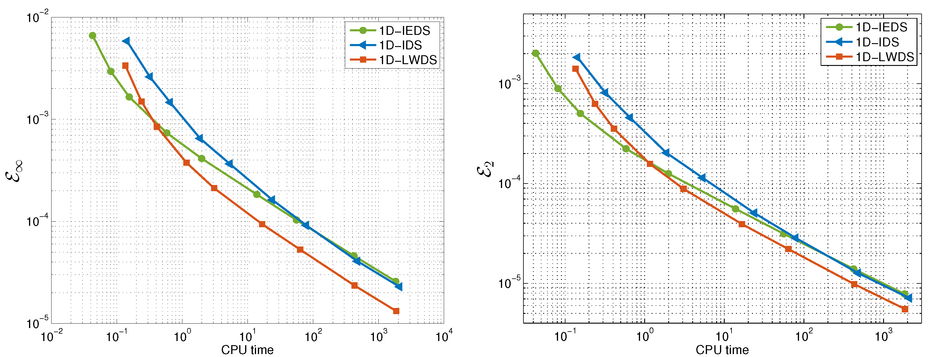
In Figure 1, we compare the errors in the maximal and $L_2$ norms versus the CPU time for all three schemes. The robustness of 1D-LWDS in contrast to 1D-IEDS and 1D-IDS is illustrated.

Note that 1D-IDS requires the building and inversion of the coefficient matrix at each time layer. Moreover, the iteration process is involved. In contrast, the coefficient matrix for both 1D-IEDS and 1D-LWDS is one and the same at each time level, and matrix inversion is necessary only once. In 1D-IEDS, the nonlinear part of the problem is computed explicitly, which leads to a loss of precision, but the performance is much faster in contrast to 1D-IDS. In 1D-LWDS, the nonlinear term is computed at a new time level but implemented in an explicit manner. Thus, the averaging technique of the Lax–Wendroff method, applied for construction of 1D-LWDS, leads to better precision and fast performance. Moreover, the computational process is more efficient than for 1D-IEDS.

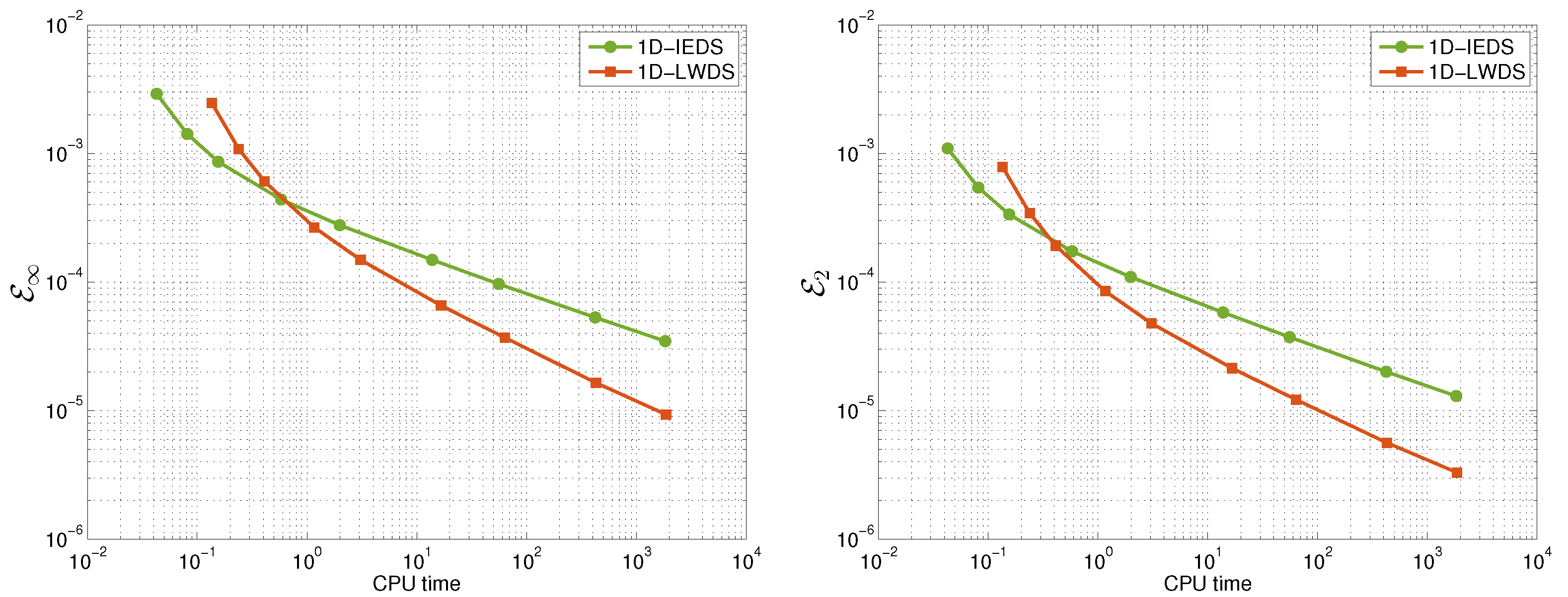
In Figure 2, we present the errors versus CPU time of 1D-IEDS and 1D-LWDS for TP2. For this test example, 1D-IDS fails as it uses the derivative of $z\left(u\right)$ at points $x=0$ and $x=a$, so division by zero is involved.

Example 2 (2D problem).

As before, we considered a test example with an exact solution. The right-hand side function, as well as the initial and boundary functions were chosen such that $u(x,y,t)=e^{t/2}(sin\left(\pi x\right)+cos(\pi y/2))$ is the exact solution of Problems (37)–(39) (TP1). The errors and orders of convergence in the maximum and $L_2$ norms were computed as follows:

$$\begin{array}{c}{\displaystyle E_{i,j}^n=u_{i,j}^n-u(x_i,y_j,t_n),}& {\displaystyle {\mathcal{E}}_{\infty }={\mathcal{E}}_{\infty }^{I,J}=\underset{1\le n\le N}{max}\underset{0\le i\le I}{max}\underset{0\le j\le J}{max}\left|E_{i,j}^n\right|,{\mathcal{E}}_2={\mathcal{E}}_2^{I,J}=\sqrt{hk\tau \sum _{i=0}^I\sum _{n=0}^J\sum _{n=1}^N{\left(E_{i,j}^n\right)}^2},}\\ {\displaystyle C{R}_{\infty }={log}_2\frac{{\mathcal{E}}_{\infty }^{I,J}}{{\mathcal{E}}_{\infty }^{2I,2J}},C{R}_2={log}_2\frac{{\mathcal{E}}_2^{I,J}}{{\mathcal{E}}_2^{2I,2J}}.}\end{array}$$

Further, all computations were performed for $I=J$, $\tau =h^2=k^2$. As in Example 1, we modified ${\mathcal{D}}_x^{+}{u}_{I-1,j}$ and ${\mathcal{D}}_x^{-}{u}_{1,j}$:

$$\begin{array}{ccc}& & {\mathcal{D}}_x^{+}{u}_{I-1,j}={\displaystyle \frac{{\left({\psi }_2\right)}_j^n-2u_{I-1,j}^n+u_{I-2,j}^n}{2h^2}}+{\displaystyle \frac{2{\left({\psi }_2\right)}_j^n-5u_{I-1,j}^n+4u_{I-2,j}^n-u_{I-3,j}^n}{2h^3}},\hfill \\ & & {\mathcal{D}}_x^{-}{u}_{1,j}={\displaystyle \frac{u_{2,j}^n-2u_{1,j}^n+{\left({\psi }_1\right)}_j^n}{2h^2}}+{\displaystyle \frac{{\left({\psi }_1\right)}_j^n-5u_{1,j}^n+4u_{2,j}^n-u_{3,j}^n}{2h^3}}.\hfill \end{array}$$

In

Table 5. The errors and spatial convergence rate of the solution, 2D problem, $\epsilon =1/2$, 2D-IEDS, $\tau =h^2$, and Example 2.

I	${\mathcal{E}}_{\mathit{\infty }}$	${\mathit{CR}}_{\mathit{\infty }}$	${\mathcal{E}}_2$	${\mathit{CR}}_2$
20	1.3364 × 10−2		1.3364 × 10−2
40	3.3351 × 10−3	2.0026	8.4541 × 10−4	3.9826
80	8.3217 × 10−4	2.0028	2.1114 × 10−4	2.0014
160	2.0807 × 10−4	1.9998	5.2774 × 10−5	2.0003
320	5.2020 × 10−5	1.9999	1.3193 × 10−5	2.0001

,

Table 6. The errors, spatial convergence rate of the solution, the averaging number of iterations, 2D problem, $\epsilon =1/2$, 2D-IDS, $\tau =h^2$, and Example 2.

I	${\mathcal{E}}_{\mathit{\infty }}$	${\mathit{CR}}_{\mathit{\infty }}$	${\mathcal{E}}_2$	${\mathit{CR}}_2$	${\mathit{m}}_{\mathbf{av}}$
20	1.0544 × 10−2		1.0544 × 10−2		2.025
40	2.6284 × 10−3	2.0041	6.6129 × 10−4	3.9949	2
80	6.5682 × 10−4	2.0006	1.6518 × 10−4	2.0013	2
160	1.6415 × 10−4	2.0005	4.1287 × 10−5	2.0002	2
320	4.1024 × 10−5	2.0005	1.0320 × 10−5	2.0002	2

and

Table 7. The errors and spatial convergence rate of the solution, 2D problem, $\epsilon =1/2$, 2D-LWDS, $\tau =h^2$, and Example 2.

I	${\mathcal{E}}_{\mathit{\infty }}$	${\mathit{CR}}_{\mathit{\infty }}$	${\mathcal{E}}_2$	${\mathit{CR}}_2$
20	3.6906 × 10−3		1.0569 × 10−3
40	9.5159 × 10−4	1.9555	2.6698 × 10−4	1.9851
80	2.4040 × 10−4	1.9849	6.6796 × 10−5	1.9989
160	6.0237 × 10−5	1.9967	1.6696 × 10−5	2.0003
320	1.5055 × 10−5	2.0004	4.1728 × 10−6	2.0004

, we give computational results of 2D-IEDS, 2D-IDS, and 2D-LWDS. The order of convergence of all three schemes is $O(\tau +h^2)$. The precision of 2D-LWDS is higher in comparison to 2D-IEDS and 2D-IDS.

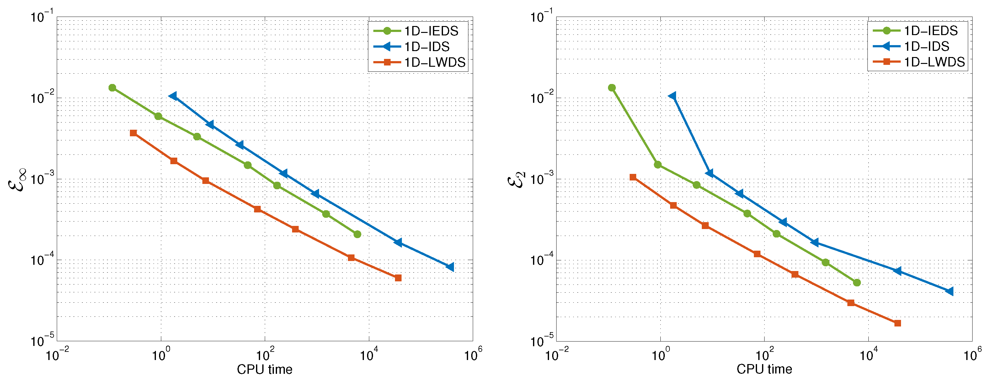
In Figure 3, we evaluate the efficiency of 2D-IEDS, 2D-IDS, and 2D-LWDS. Clearly, 2D-LWDS achieves higher precision with shorter computational time compared to both 2D-IEDS and 2D-IDS.

The stability of the proposed approach is ensured by Condition (22). In practice, however, this restriction tends to be somewhat relaxed. For instance, in the present example, the method remains stable for $\tau =3h^2$.

7. Conclusions

We considered three numerical methods for solving 1D and 2D nonlinear pseudoparabolic problems—implicit scheme (1D-IDS and 2D-IDS), implicit–explicit schemes (1D-EIDS and 2D-IEDS), and Lax–Wendroff-type discretizations (1D-LWDS and 2D-LWDS). All these methods are first-order accurate in time and second-order in space, both in the maximal and $L_2$ norms.

In the stability region, 1D-LWDS and 2D-LWDS are more efficient compared to the 1D-IDS, 2D-IDS, and 1D-EIDS, 2D-IEDS methods, respectively. The disadvantage of the Lax–Wendroff type schemes is that their stability condition is similar to that of explicit schemes when solving parabolic equations.

In this paper, we demonstrated that the Lax–Wendroff method can be effectively applied for the numerical solution of pseudoparabolic equations with a nonlinear flux. The method proposed in our work is both iteration-free and applicable to a general class of nonlinear fluxes. If higher-order spatial approximation methods are employed to derive the underlying difference equations in our Lax–Wendroff scheme, the order of convergence in space for the resulting Lax–Wendroff discretization would increase. Moreover, in such cases, using a $O\left({\tau }^2\right)$ truncation of the solution at half time layers, which is a base of the explicit flux approximation, would also enhance the temporal convergence order. The development and analysis of a high-order Lax–Wendroff scheme for solving nonlinear pseudoparabolic equations will be the focus of our future research.

Overall, this research contributes to advancing numerical techniques that can be extended to solve time-fractional pseudoparabolic equations with a nonlinear flux.