Article

The Effects of the Weak Allee Effect and Disease on the Dynamics of a Predator–Prey System: Stability and Bifurcation Properties

1
School of Mathematics and Computer Science, Northwest Minzu University, Lanzhou 730030, China
2
Experimental Teaching Department, Northwest Minzu University, Lanzhou 730030, China
*
Author to whom correspondence should be addressed.
Axioms 2025, 14(7), 531; https://doi.org/10.3390/axioms14070531
Submission received: 7 June 2025 / Revised: 5 July 2025 / Accepted: 8 July 2025 / Published: 12 July 2025

Abstract

In this paper, an eco-epidemiological model with a weak Allee effect and prey disease dynamics is discussed. Mathematical features such as non-negativity, boundedness of solutions, and local stability of the feasible equilibria are discussed. Additionally, the transcritical bifurcation, saddle-node bifurcation, and Hopf bifurcation are proven using Sotomayor’s theorem and Poincare–Andronov–Hopf theorems. In addition, the correctness of the theoretical analysis is verified by numerical simulation. The numerical simulation results show that the eco-epidemiological model with a weak Allee effect has complex dynamics. If the prey population is not affected by disease, the predator becomes extinct due to a lack of food. Under low infection rates, all populations are maintained in a coexistent state. The Allee effect does not influence this coexistence. At high infection rates, if the prey population is not affected by the Allee effect, the infected prey is found to coexist in an oscillatory state. The predator population and the susceptible prey population will be extinct. If the prey population is affected by the Allee effect, all species will be extinct.

1. Introduction

Population dynamics is a significant research domain within biomathematics. Its research plays a crucial role in maintaining ecosystem balance, conserving endangered species, and advancing ecological theory [1]. Many scholars are dedicated to exploring the interactions between populations. Since the foundational predator–prey model formulated by Lotka and Volterra [2,3], substantial research has been conducted on this model. However, interactions among populations can facilitate the spread of diseases. Considering the prevalence of diseases across multiple populations is a comprehensive application of both population dynamics and infectious disease dynamics, representing another research direction in biological mathematics known as eco-epidemiology [4,5]. Eco-epidemiological models can not only explore the impact of diseases on population coexistence and the ecological environment but also prevent the spread of diseases by regulating the living environment of the population. Anderson and May were the first researchers to use eco-epidemiological models to study the effects of diseases on ecological communities [6]. They are recognized as the pioneers in the field of eco-epidemiological modeling. Subsequently, many researchers combined epidemiology with population dynamics to establish many mathematical models of eco-epidemiology based on the principle of population dynamics and the mechanism of epidemiological modeling.
In order to make the model more in line with the actual ecological significance, modifying the model is usually considered. For example, the Allee effect describes the positive correlation between individual fitness and population density at low density [7,8,9,10,11,12,13]. It can be categorized into two types: strong and weak Allee effects. The weak Allee effect occurs when there is a positive correlation between individual fitness and population density at low densities, but this correlation disappears or becomes negligible at higher densities. This means that while populations experiencing a weak Allee effect may grow more slowly at low densities, they do not face an immediate risk of extinction due to the effect alone. The primary factors contributing to the Allee effect include challenges associated with mate selection, the negative consequences of inbreeding, impaired social functioning within small communities, the need for predator avoidance, and the exploitation of limited food resources [14,15]. A large amount of experimental evidence has shown that the Allee effect is widespread in many species in nature [10,11,12,13,16,17]. For example, in arthropods, the Glanville fritillary butterfly [18,19] and Monarch butterfly [18,20] have fewer mating opportunities due to the scarcity of individuals, which in turn reduces the reproductive success rate of the population. Social spiders [21] exhibit reduced resistance to predators and impaired resource acquisition under low-density conditions, leading to decreased offspring survival rates. Among mammals, African wild dogs [20], desert bighorn sheep [22], meerkat [18,23], and woodland caribou [18,23] cannot effectively cooperate to defend predators due to small groups, resulting in an increase in individual mortality. In mollusks, queen conch [24] and snail [24] rely on pheromone signals in the process of finding spouses. If the density of the population is too low, it will lead to fewer pheromone signals and it is difficult to find a suitable spouse. In avian species such as lesser kestrel, speckled warbler, and sooty shearwater [18,25], reduced collective defense capabilities under conditions of insufficient population size result in impaired detection efficiency of raptors or mammalian predators. The cases above demonstrate that the Allee effect plays a crucial role in the survival and reproduction of populations. Due to its key role in species survival, invasion, and evolution, the Allee effect has become a focus in ecology, invasion biology, and conservation biology [26]. Thus, it is essential to study the effects of the Allee effect on population dynamics and persistence.
In addition, disease is considered to be one of the main factors leading to species extinction. When disease interacts with the Allee effect, this association has important biological significance in nature. Many species are simultaneously influenced by the Allee effect and disease in natural ecosystems. The synergistic effects of these two factors have been well-documented, particularly in species such as African wild dogs [26,27,28,29] and foxes [30,31]. At present, many researchers have discussed the combined effects of the Allee effect and disease on predator–prey systems. For example, Wang et al. [26] investigated an eco-epidemiological model in which predators are infected and exhibit Allee effects. The results indicate that when the cooperation coefficient is high, the Allee effect can prevent predator extinction. Shaikh, Das et al. [11] discussed an eco-epidemiological model in which the predator was diseased and the prey experienced the Allee effect. The results showed that the Allee effect may destroy the stability of the system and cause chaotic dynamics. Saifuddin et al. [32] analyzed the eco-epidemiology of predators with different capture coefficients and a weak Allee effect. It was found that the Allee effect could regulate the chaotic dynamics of the system. Further references on the study of Allee effects in eco-epidemiological models can be found in [33,34,35,36]. Therefore, it is of great significance to understand the combined effects of the Allee effect and disease on predator–prey interaction, which is helpful to deepen the understanding of species diversity and disease outbreak mechanisms.
The role of the Allee effect in eco-epidemiological models has been widely studied. Studies have shown that reduced contact between species at low population densities may inhibit disease transmission or affect species persistence. In this paper, a novel eco-epidemiological model was developed to focus on the predator–prey system with infected prey populations. This model adopts the same form of weak Allee effect characterization function as in Refs. [9,12,15]. It follows the law of mass action for interactions between susceptible and infected prey and adheres to the Holling type I functional response for interactions between infected prey and predators. The aim is to characterize the exposed state of prey that have become physically weakened by infection and lost their ability to actively avoid predation.
Compared with most studies focusing on the strong Allee effect, this paper deeply discusses the bidirectional effects of the weak Allee effect coupled with disease dynamics in a predator–prey system. The hypothesis breaks through the assumption of indiscriminate predation by predators to fit the actual ecological scenario (where diseases affect the activity status of prey), enabling the model to more accurately characterize the linkage among diseases, the Allee effect, and predation relationships. This provides a unique foundation for subsequent stability and bifurcation analyses.
In this paper, the weak Allee effect and disease transmission rate are taken as the main research factors. The influence of disease transmission rate on the population is explored when the prey population is not affected by the weak Allee effect. Additionally, how the weak Allee effect affects population growth is analyzed when there is no disease transmission among populations. The dynamic behavior of the model is investigated under the conditions where the prey population is affected by both the Allee effect and diseases and the predator has no other food sources (relying solely on infected prey). This modeling assumption is based on the biological mechanism that diseases may reduce the mobility of prey, making them more susceptible to predation. Through a qualitative analysis of the model under conditions of coexisting Allee effect and diseases, the conditions for the stable coexistence of susceptible prey, infected prey, and predators are revealed.
The rest of this article is arranged as follows: Section 2 introduces the establishment of the model and related assumptions; Section 3 discusses the dynamics of the model in detail. In Section 4, the theoretical results are verified by numerical simulation. Section 5 gives a brief summary.

2. Mathematical Model Formulation

An eco-epidemiological model incorporating prey disease and the weak Allee effect was developed and is discussed in this section. To facilitate mathematical analysis, the following assumptions were made.
  • Assuming that there is no predator in the system, the dynamics of the prey population is described by the logistic equation, i.e., d N d t = r N ( 1 N K ) , where r is the intrinsic growth rate and K is the environmental carrying capacity.
  • In the presence of disease, we divide the prey population into two subclasses and use S and I to represent susceptible prey and infected prey, respectively.
  • The disease transmission is confined to the prey population. Infected prey dies before attaining reproductive capability and cannot recover from the infection.
  • The predator only captures the diseased prey, because the activity of the diseased prey may be weakened, and it is easy to be captured.
Therefore, based on the above assumptions, the eco-epidemiological model for infected prey with a weak Allee effect can be expressed by the following nonlinear differential equation:
d S ( t ) d t = r S ( t ) ( 1 S ( t ) + I ( t ) K ) S ( t ) S ( t ) + A β S ( t ) I ( t ) , d I ( t ) d t = β S ( t ) I ( t ) d I ( t ) c I ( t ) P ( t ) , d P ( t ) d t = e ( c I ( t ) P ( t ) ) m P ( t ) ,
with initial conditions
S 0 = S ( 0 ) > 0 ,   I 0 = I ( 0 ) 0 ,   P 0 = P ( 0 ) 0 ,
where S ( t ) , I ( t ) , and P ( t ) denote the population densities of the susceptible prey, the infected prey, and the predator at time t, respectively. The Allee effect is described by the function S S + A , representing the probability of mate finding. A denotes the reciprocal of individual search efficiency [9,23]. We assume that the contact between crowds is random; that is, each individual has an equal chance of contact, where β represents the probability that each infected person infects the susceptible person in a unit time. c denotes the attack rate of the predator on the diseased prey; e denotes the conversion efficiency of the predator to the prey, d denotes the mortality rate of the infected prey; and m denotes the natural mortality rate of predators without prey. All variables and parameters are positive.
Next, we illustrate the ecological significance of the model; that is, the solution of model (1) is positive and bounded.
The consideration of population positivity is a crucial assumption in ecological models. The primary reason for this is that, in real ecosystems, population sizes cannot be negative or zero. Negative population sizes are biologically meaningless and cannot represent any actual biological entities or quantities.
Theorem 1.
When t 0 , the solution ( S , I , P ) of model (1) is positive for any initial value ( S 0 , I 0 , P 0 ) R + 3 .
S ( t ) = S ( 0 ) exp 0 t r ( 1 S ( s ) + I ( s ) K ) S ( s ) S ( s ) + A β I ( s ) d s > 0 , I ( t ) = I ( 0 ) exp 0 t β S ( s ) d c P ( s ) d s 0 , P ( t ) = P ( 0 ) exp 0 t e c I ( s ) m d s 0 .
The boundedness of populations is considered very important in ecological models. In nature, no population can grow infinitely due to resource limitations. In constructing mathematical models, if unlimited population growth is allowed, it may lead to instability of the model solutions. The mathematical reliability and biological rationality of the model cannot be guaranteed. The following theorem mainly guarantees that the population cannot grow infinitely.
Theorem 2.
The set Ω is positive invariant, and all solutions of the model (1) are ultimately bounded within the region.
Proof. 
For any S t 0 , I t 0 , and P t 0 , we can derive
d S ( t ) d t | S = 0 = 0 ,   d I ( t ) d t | I = 0 = 0 ,   d P ( t ) d t | P = 0 = 0 ,
which implies that S = 0 , I = 0 , and P = 0 are invariant manifolds. It then follows that the model (1) is positively invariant in R + 3 . Since
d S ( t ) d t = r S ( t ) ( 1 S ( t ) + I ( t ) K ) S ( t ) S ( t ) + A β S ( t ) I ( t ) r S ( t ) ( 1 S ( t ) K ) ,
following directly from Lemma 2.2 [32], it is easy to see that
lim sup t   S ( t ) K .
Define L t = S t + I t + 1 e P t , and the derivative of L t is
d L t d t + δ L t = d S t d t + d I t d t + 1 e d P t d t + δ L t = r S ( 1 S + I K ) S S + A + δ S + I ( δ d ) + ( δ e m e ) P ( r + δ ) S r K S 2 + I ( δ d ) + ( δ e m e ) P ,
Let 0 δ min d , m ; we have
d L d t + δ L ( r + δ ) S r K S 2 K ( r + δ ) 2 4 r : = F .
By using the comparison principle, we have
L t F δ + L ( 0 ) F δ e δ t , t 0 .
It is easy to get that L t F δ as t . Thus, all solutions of model (1) starting in R + 3 will be confined within the region
Ω : = ( S , I , P ) R + 3 : 0 S + I + 1 e P F δ .

3. Dynamics of the Model

3.1. Equilibrium Existence

Following [37,38], we obtain the basic reproduction number 0 for model (1) as follows:
0 = β K d .
It is easy to calculate that model (1) has the following equilibrium point:
  • Trivial equilibrium E 0 = 0 , 0 , 0 , which always exists.
  • Axial equilibrium E 1 = K , 0 , 0 , which always exists.
  • Planar equilibrium E 2 = S ¯ , I ¯ , 0 exists when K > d β , with its components as S ¯ = d β , I ¯ = r S ¯ ( K S ¯ ) β K S ¯ + r S ¯ + A β K .
E 0 = 0 , 0 , 0 represents the state where the ecosystem has completely collapsed, indicating that no species can survive. E 1 = K , 0 , 0 indicates that there are no diseases or predators in the system, reflecting the maximum population size that the susceptible prey can reach under resource constraints. E 2 = S ¯ , I ¯ , 0 represents the equilibrium state reached by the spread of the disease in the prey population in a system without a predator population. That is, E 2 = S ¯ , I ¯ , 0 , and its dynamical behavior degenerates to the classic SI model.
Next, the existence of the coexistence equilibrium of the model is analyzed, and E satisfies the following equation:
r ( 1 S ( t ) + I ( t ) K ) S ( t ) S ( t ) + A β I ( t ) = 0 , β S ( t ) d c P ( t ) = 0 , e c I ( t ) m = 0 ,
which yields I = m e c , and S is the positive root of the following equation:
G ( S ) = l 1 S 2 + l 2 S + l 3 = 0 ,
where l 1 = e c r > 0 , l 2 = ( K m β + r m e c r K ) , and l 3 = A m β K > 0 .
If l 2 = ( K m β + r m e c r K ) < 0 and Δ = [ K ( m β e c r ) + r m ] 2 4 e c r A m β K > 0 are satisfied, the function G ( S ) has two positive roots S 1 and S 2 by calculation. The coexistence equilibrium exists if l 2 < 0 , Δ > 0 and both of the solutions satisfy S 1 > d β , S 2 > d β .
S 1 = K e c r K m β r m [ K ( m β e c r ) + r m ] 2 4 e c r A m β K 2 e c r ,   P 1 = β S 1 d c .
S 2 = K e c r K m β r m + [ K ( m β e c r ) + r m ] 2 4 e c r A m β K 2 e c r ,   P 2 = β S 2 d c .
Under certain conditions, these two equilibrium points will coincide as the only positive equilibrium point E = ( S , I , P ) . Now,
S = K e c r K m β r m 2 e c r ,   P = β S d c ,
when l 2 2 4 l 1 l 3 0 is equivalent to A [ K ( m β e c r ) + r m ] 2 4 e c r m β K .
In summary, the existence conditions of the coexistence equilibrium point of model (1) are obtained and summarized as the following theorem.
Theorem 3.
The existence of the coexistence equilibrium point of model (1) is as follows:
a. 
Model (1) does not have a coexistence equilibrium if and only if one of the following conditions holds:
(a) 
A > [ K ( m β e c r ) + r m ] 2 4 e c r m β K ;
(b) 
A [ K ( m β e c r ) + r m ] 2 4 e c r m β K  and  ( K m β + r m e c r K ) > 0 ;
b. 
If conditions   ( K m β + r m e c r K ) < 0   and   A = [ K ( m β e c r ) + r m ] 2 4 e c r m β K   hold, then   G ( S )   has exactly one real positive root. Therefore, the model has one coexistence equilibrium  E = ( S , I , P ) .
c. 
If conditions  ( K m β + r m e c r K ) < 0  and  A < [ K ( m β e c r ) + r m ] 2 4 e c r m β K  are satisfied, then  G ( S )  has two real positive roots. Therefore, the model has two coexistence equilibria  E 1 = ( S 1 , I , P 1 )  and   E 2 = ( S 2 , I , P 2 ) .

3.2. Local Stability Analysis

Analyzing the stability of equilibrium points helps reveal the model’s long-term dynamics. Next, the local stability of the boundary equilibrium points and coexistence equilibrium points will be discussed.
Theorem 4.
The stability of the boundary equilibrium point is summarized as follows:
a. 
E 0  is a saddle node.
b. 
E 1  is locally asymptotically stable if  β K < d R 0 < 1 . Otherwise, it is unstable.
c. 
If  e c I ¯ m < 0  and   C 11 < 0  are satisfied, then  E 2   is locally asymptotically stable; conversely, it is unstable.
Proof. 
The generalized Jacobian matrix is presented in Appendix A. Meanwhile, the Jacobian matrices corresponding to all equilibrium points have also been derived and calculated.
Through the derivation in Appendix A, the three characteristic roots of J ( E 0 ) can be directly obtained, which are λ 1 = 0 , λ 2 = d , and λ 3 = m . Based on the properties of the aforementioned characteristic roots, E 0 can be determined to be a saddle node. Similarly, following the derivation logic in Appendix A, it can be further deduced that there exist three characteristic roots for J ( E 1 ) , which are λ 1 = m , λ 2 = r K K + A , and λ 3 = β K d . Thus, E 1 is stable if β K < d R 0 < 1 holds. Otherwise, it is unstable.
Based on the derivation content in Appendix A, the characteristic equation corresponding to E 2 can be constructed, and its specific form is as follows:
( λ ( e c I ¯ m ) ) ( λ 2 C 11 λ C 21 C 12 ) = 0 ,
It can be directly deduced that C 21 C 12 < 0 . If e c I ¯ m < 0 and C 11 < 0 are satisfied, then E 2 is locally asymptotically stable; conversely, it is unstable. □
Theorem 5.
The stability of the coexistence equilibrium point is summarized as follows:
a. 
If  S > S +  holds, then the unique coexistence equilibrium  E  is stable; otherwise, it is unstable.
b. 
If  S 1 > S +  holds, then the coexistence equilibria  E 1  and  E 2  are both locally asymptotically stable.
c. 
If  S 1 < S + < S 2  holds, then the coexistence equilibrium  E 2  is stable, while  E 1  remains unstable.
Proof. 
From the Jacobian matrix of E given in Appendix A, the corresponding characteristic equation can be written:
λ 3 + B 2 ( E ) λ 2 + B 1 ( E ) λ + B 0 ( E ) = 0 ,
where B 2 ( E ) = c 11 , B 1 ( E ) = ( c 12 c 21 + c 23 c 32 ) > 0 , and B 0 ( E ) = c 11 c 23 c 32 . Based on the Routh–Hurwitz criterion, if B 2 > 0 , B 0 > 0 , and B 2 B 1 B 0 > 0 hold simultaneously, all roots of Equation (4) have negative real parts, and E is locally asymptotically stable. Conversely, if any condition is not satisfied, then E loses stability.
Since the signs of c 12 , c 21 , c 23 , and c 32 are fixed, we focus on how c 11 affects the stability of the coexistence equilibrium.
Let f ( S ) = r S S 2 2 A S + A ( K m e c ) and c 11 = f ( S ) K ( S + A ) 2 . Analytically, f S has three roots: S = 0 , S = 2 A Δ 1 2 < 0 , and S + = 2 A + Δ 1 2 > 0 ( Δ 1 = 4 A 2 + 4 A ( K m / e c ) ). Its derivative f S = 3 r S 2 4 r A S + r A ( K m e c ) has two roots: S = 2 A + Δ 2 3 < 0 and S + = 2 A Δ 2 3 > 0 ( Δ 2 = 4 A 2 + 3 A ( K m / e c ) ), satisfying S + > S + and S > S . Thus, f S 0 on 0 , S + and f S < 0 on S + , + . By comparing the numerical magnitudes of S , S 1 , S 2 , and S + , the sign of c 11 can be further determined.
Next, the stability of the model will be analyzed in two cases: (1) the stability of the unique coexistence equilibrium point; (2) the stability of the two coexistence equilibrium points when certain conditions are satisfied.
  • Case (1)
If K e c r K m β r m 2 e c r > A + A 2 + A ( K m e c ) holds, then c 11 ( E ) < 0 , which means that the Routh–Hurwitz conditions B 2 ( E ) B 1 ( E ) B 0 ( E ) = c 11 c 12 c 21 > 0 , B 2 ( E ) > 0 , and B 0 ( E ) > 0 are satisfied, and it can be inferred that E is locally asymptotically stable.
  • Case (2)
If K e c r K m β r m [ K ( m β e c r ) + r m ] 2 4 e c r A m β K 2 e c r > A + A 2 + A ( K m e c ) holds, then c 11 ( E 1 ) < 0 , c 11 ( E 2 ) < 0 ; thus equilibria E 1 and E 2 are both locally asymptotically stable. If S 1 < S + < S 2 holds, E 1 remains unstable while equilibrium E 2 remains stable. □

3.3. Bifurcation Analysis

3.3.1. Transcritical Bifurcation

Transcritical bifurcation occurs when a model parameter crosses a critical threshold, causing two equilibrium points to exchange stability. This phenomenon typically describes the transition from disease extinction to endemic persistence in populations. The following theorem describes the occurrence of a transcritical bifurcation in model (1).
Theorem 6.
Model (1) undergoes transcritical bifurcation at the axial equilibrium E 1 when it goes through the critical value β = β = d K and satisfies the following conditions:
W T f β ( E 1 , β ) = 0 ,   W T D f β ( E 1 , β ) V 0 ,   W T D 2 f ( E 1 , β ) V , V 0 .
Proof. 
We use Sotomayor’s theorem to analyze the dynamics of the model in the neighborhood of the equilibrium point E 1 , since J ( E 1 ) has a zero eigenvalue when β = β . Let V and W be the eigenvectors corresponding to the zero eigenvalues of J ( E 1 ) and J ( E 1 ) T , respectively, where
J ( E 1 , β ) = a 11 a 12 0 0 0 0 0 0 a 33 ,   J ( E 1 , β ) T = a 11 0 0 a 12 0 0 0 0 a 33 ,
Here, a 11 = r K ( K + A ) , a 12 = r K ( K + A ) β K , a 33 = m . V T = 1 , a 11 a 12 , 0 , and W T = 0 , a 12 a 11 , 0 can be obtained by simple calculation.
Now,
f β ( E 1 , β ) = 0 0 0 T = 0 , D f β ( E 1 , β ) V = 0 K 0 0 K 0 0 0 0 1 a 11 a 12 0 = a 11 K a 12 a 11 K a 12 0 T .
D 2 f ( E 1 , β ) V , V = g 11 0 0 g 14 0 0 0 0 0 g 24 0 g 26 0 0 0 0 0 g 36 V 1 2 V 2 2 V 3 2 2 V 1 V 2 2 V 1 V 3 2 V 2 V 3 = V 1 2 g 11 + 2 V 1 V 2 g 14 2 V 1 V 2 g 24 + 2 V 2 V 3 g 26 2 V 2 V 3 g 36 ,
where
g 11 = 4 r K + A 10 r K K + A 2 , g 14 = 2 r K + A + r K K + A 2 β , g 24 = β , g 26 = c , g 36 = e c .
Thus,
W T f β ( E 1 , β ) = 0 ,   W T D f β ( E 1 , β ) V = 0 , a 12 a 11 , 0 a 11 K a 12 a 11 K a 12 0 = K 0 ,
W T D 2 f ( E 2 , β ) V , V = 0 , a 12 a 11 , 0 V 1 2 g 11 + 2 V 1 V 2 g 14 2 V 1 V 2 g 24 + 2 V 2 V 3 g 26 2 V 2 V 3 g 36 = 2 V 1 V 2 g 24 a 12 a 11 = 2 β 0 .
The proof is completed. □
From an ecological perspective, when the parameter satisfies β < β , it indicates that the disease transmission ability is relatively weak and the growth of infected prey is small. This will further reduce the food sources for predators. As time evolves dynamically, only susceptible prey will ultimately remain in the system. When the parameter satisfies β > β , it shows that the disease transmission ability is relatively strong and the growth rate of infected prey is fast. This will further accelerate the growth of predators; that is, the system will ultimately reach a state of coexistence of three species.

3.3.2. Saddle-Node Bifurcation

According to Theorem 3, when ( K m β + r m e c r K ) < 0 and A < [ K ( m β e c r ) + r m ] 2 4 e c r m β K , the model has two equilibrium points. When ( K m β + r m e c r K ) < 0 and A = [ K ( m β e c r ) + r m ] 2 4 e c r m β K , the two positive equilibrium points coincide. When A > [ K ( m β e c r ) + r m ] 2 4 e c r m β K , the positive equilibrium point disappears. The appearance or disappearance of the equilibrium point is due to the existence of a saddle-node bifurcation at E . The following theorem describes the occurrence of a saddle-node bifurcation in model (1).
Theorem 7.
Model (1) undergoes saddle-node bifurcation at E when it goes through the critical value A = A S N = [ K ( m β e c r ) + r m ] 2 4 e c r m β K and satisfies the following conditions:
M T f A ( E , A S N ) 0 ,   M T D 2 f ( E , A S N ) H , H 0 .
Proof. 
We use Sotomayor’s theorem in order to establish the dynamics of the model in the neighborhood of the equilibrium point E , since J ( E ) has a zero eigenvalue at A = A S N .
Let H and M be the eigenvectors corresponding to the zero eigenvalues of J ( E ) and J ( E ) T , respectively, where
J ( E , A = A S N ) = c 11 S N c 12 S N 0 c 21 S N 0 c 23 S N 0 c 32 S N 0 ,   J ( E , A = A S N ) T = c 11 S N c 21 S N 0 c 12 S N 0 c 32 S N 0 c 23 S N 0 .
Based on λ 3 + B 2 ( E ) λ 2 + B 1 ( E ) λ + B 0 ( E ) = 0 , we have λ 1 λ 2 λ 3 = B 0 ( E ) .To ensure that any one of the eigenvalues is zero, it is necessary to satisfy B 0 ( E ) = 0 ; that is c 11 S N = 0 . Therefore, we can calculate H T = 1 , 0 , c 21 S N c 32 S N and M T = 1 , 0 , c 12 S N c 32 S N .
Then,
f A ( E , A S N ) = r S 2 [ K ( S + I ) ] K ( S + A S N ) 2 0 0 T 0 ,
D 2 f ( E , A S N ) H , H = l 11 0 0 l 14 0 0 0 0 0 l 24 0 l 26 0 0 0 0 0 l 36 H 1 2 H 2 2 H 3 2 2 H 1 H 2 2 H 1 H 3 2 H 2 H 3 = H 1 2 l 11 + 2 H 1 H 2 l 14 2 H 1 H 2 l 24 + 2 H 2 H 3 l 26 2 H 2 H 3 l 36 ,
where
l 11 = 2 r K ( 6 r S + 2 r I ) K S + A S N + 2 ( 3 r S 2 + 2 r S I 2 r S K ) K S + A S N 2 + 2 ( r S 2 K r S 3 r S 2 I ) K S + A S N 3 ,
l 14 = 2 r S K S + A S N + r S 2 K S + A S N 2 β ,   l 24 = β ,   l 26 = c ,   l 36 = e c .
Thus,
M T f A ( E , A S N ) = 1 , 0 , c 12 S N c 32 S N r S 2 [ K ( S + I ) ] K ( S + A S N ) 2 0 0 T = r S 2 [ K ( S + I ) ] K ( S + A S N ) 2 0 ,
M T D 2 f ( E , A S N ) H , H = 1 , 0 , c 12 S N c 23 S N H 1 2 l 11 + 2 H 1 H 2 l 14 2 H 1 H 2 l 24 + 2 H 2 H 3 l 26 2 H 2 H 3 l 36 = H 1 2 l 11 = l 11 0 .
Therefore, Sotomayor’s theorem confirms that a saddle-node bifurcation occurs in model (1) as parameter A crosses the critical value A S N . □
When the parameter A < A S N , the system exhibits two coexisting equilibrium points: one is a stable point and the other is an unstable point. At the bifurcation point A = A S N , this coexisting equilibrium point (semi-stable state) is defined as a saddle node. When A > A S N , the coexisting equilibrium points disappear, indicating that the three species cannot achieve coexistence. Under the influence of the weak Allee effect, in a low-density environment, the prey population struggles to effectively complete ecological processes such as mating behavior and collaborative resistance against disease transmission and predation pressure. Consequently, their survival and reproductive processes are inhibited. Therefore, to ensure the survival of the three species under disease transmission conditions, the prey population must be strictly maintained above the low-density threshold.

3.3.3. Hopf Bifurcation

This section presents a systematic analysis of potential Hopf bifurcation phenomena occurring in the neighborhood of the equilibrium point E . As established by Theorem 5, when the parameters satisfy B 2 B 1 B 0 = 0 , the characteristic Equation (4) yields a pair of conjugate purely imaginary roots. Under this condition, the stability of E undergoes a critical transition. The emergence of this critical state constitutes a necessary condition for Hopf bifurcation to occur in the vicinity of E .
Theorem 8.
Model (1) has a Hopf bifurcation around E when β passes through β H provided B 2 β H B 1 β H = B 0 β H .
Proof. 
At β = β H , the characteristic equation λ 3 + B 2 λ 2 + B 1 λ + B 0 = 0 can be factorized as ( λ 2 + B 1 ) ( λ + B 2 ) = 0 . It is easy to analyze that there is a pair of conjugate pure imaginary roots λ 1 , 2 = ± i B 1 and a negative root λ 3 = B 2 .
Now verify the transversality condition
d d β e ( λ 1 , 2 ) | β = β H = d z 1 d β | β = β H 0 .
Putting λ = z 1 + i z 2 into λ 3 + B 2 λ 2 + B 1 λ + B 0 = 0 , and then taking the derivative of β, we can get
3 ( z 1 + i z 2 ) 2 ( z 1 + i z 2 ) + B 2 ( z 1 + i z 2 ) 2 + 2 B 2 ( z 1 + i z 2 ) ( z 1 + i z 2 ) + B 1 ( z 1 + i z 2 ) + B 1 ( z 1 + i z 2 ) + B 0 = 0 .
By separating the real part and the imaginary part, the following linear equations can be obtained.
G 1 z 1 + G 2 z 2 + H 1 = 0 , G 3 z 1 + G 4 z 2 + H 2 = 0 , ,
where
G 1 = 3 z 1 2 3 z 2 2 + 2 B 2 z 1 + B 1 , G 2 = 6 z 1 z 2 2 B 2 z 2 , H 1 = B 2 z 1 2 B 2 z 2 2 + B 1 z 1 + B 0 , G 3 = 6 z 1 z 2 + 2 B 2 z 2 , G 4 = 3 z 1 2 3 z 2 2 + 2 B 2 z 1 + B 1 , H 2 = 2 z 1 z 2 B 2 + B 1 z 2 .
It follows from (5) that
z 1 = H 2 G 2 H 1 G 4 G 4 G 1 G 3 G 2 .
We know that when the Hopf bifurcation occurs, the characteristic equation λ 3 + B 2 λ 2 + B 1 λ + B 0 = 0 has a pair of purely imaginary roots λ 1 , 2 = ± i B 1 ; that is z 1 = 0 , z 2 = B 1 or z 2 = B 1 . In order to show that the transversality condition holds, we consider whether H 2 G 2 H 1 G 4 and G 4 G 1 G 3 G 2 are zero at β = β H in the following two cases.
Case 1 z 1 = 0 , z 2 = B 1 . We obtain
G 1 = 2 B 1 ,   G 2 = 2 B 2 B 1 ,   G 3 = 2 B 2 B 1 ,   G 4 = 2 B 1 ,
H 1 = B 2 B 1 + B 0 ,   H 2 = B 1 B 1 > 0 .
Therefore, from (5)
z 1 = H 2 G 2 H 1 G 4 G 4 G 1 G 3 G 2 = B 1 ( 2 B 0 2 B 2 B 1 2 B 1 B 2 ) 4 B 1 2 ( B 2 2 1 ) .
Hence, if z 1 = 0 , z 2 = B 1 , then 2 B 0 2 B 2 B 1 2 B 1 B 2 0 and B 2 2 1 0 at β = β H . Model (1) possesses a Hopf bifurcation.
Case 2 z 1 = 0 , z 2 = B 1 . We obtain
G 1 = 2 B 1 ,   G 2 = 2 B 2 B 1 ,   G 3 = 2 B 2 B 1 ,   G 4 = 2 B 1 ,
H 1 = B 2 B 1 + B 0 ,   H 2 = B 1 B 1 < 0 .
Therefore,
z 1 = H 2 G 2 H 1 G 4 G 4 G 1 G 3 G 2 = B 1 ( 2 B 0 2 B 1 B 2 2 B 2 B 1 ) 4 B 1 2 ( 1 B 2 2 ) .
Hence, if z 1 = 0 , z 2 = B 1 , then 2 B 0 2 B 2 B 1 2 B 1 B 2 0 and 1 B 2 2 0 at β = β H . Model (1) possesses a Hopf bifurcation.
In short, the conditions 2 B 0 2 B 2 B 1 2 B 1 B 2 0 and B 2 2 1 hold, and the model will have a Hopf bifurcation at the equilibrium E . □
When a parameter in the system reaches the Hopf bifurcation critical point, the originally stable population state will be disrupted, and the population size will exhibit periodic fluctuations. When the parameters satisfy that the β < β H population is stable, the smaller infection rate can ensure the stable state of the system. When β = β H , the periodic fluctuations in predators and prey introduce temporal dynamics into the ecosystem, creating differential survival and reproductive opportunities for species across time. When β > β H , a higher infection rate drives rapid disease spread. In the short term, the predator population may increase due to abundant infected prey; however, the growth rate of susceptible prey will be outpaced by disease transmission, leading to prey extinction. Subsequently, predator populations will also collapse due to energy resource depletion.

4. Numerical Simulation

We perform numerical simulations to verify the results of the mathematical analysis of model (1). The simulation is completed by using software MATLAB R2017a. In this paper, the disease transmission rate β and the Allee effect A are the key research parameters. We examine the dynamic behavior of model (1) under different disease transmission rates and Allee effect values. The time series diagram, phase plane diagram, one-parameter bifurcation diagram, and two-parameter bifurcation diagram are provided to compare the analysis results. In this paper, local stability and Hopf bifurcation are investigated. Additionally, various complex dynamic behaviors, including saddle-node bifurcation and transcritical bifurcation, are analyzed. To facilitate numerical simulations, a set of parameter values was selected:
r = 2.65 ;   K = 180 ;   c = 0.24 ;   e = 0.35 ;   d = 0.03 ;   m = 0.9
The impact of two key parameters β and A on the stability of the feasible equilibrium and the persistence of the disease is discussed below. Numerical simulations are performed by varying the values of β and A based on the parameters selected from Equation (6). Figure 1 shows that the smaller infection rate ensures the existence of the coexistence equilibrium point, and the coexistence equilibrium point can be stabilized by combining with the appropriate Allee effect value. In other words, in order to make all species in the system coexist, the disease must be prevalent in the system.
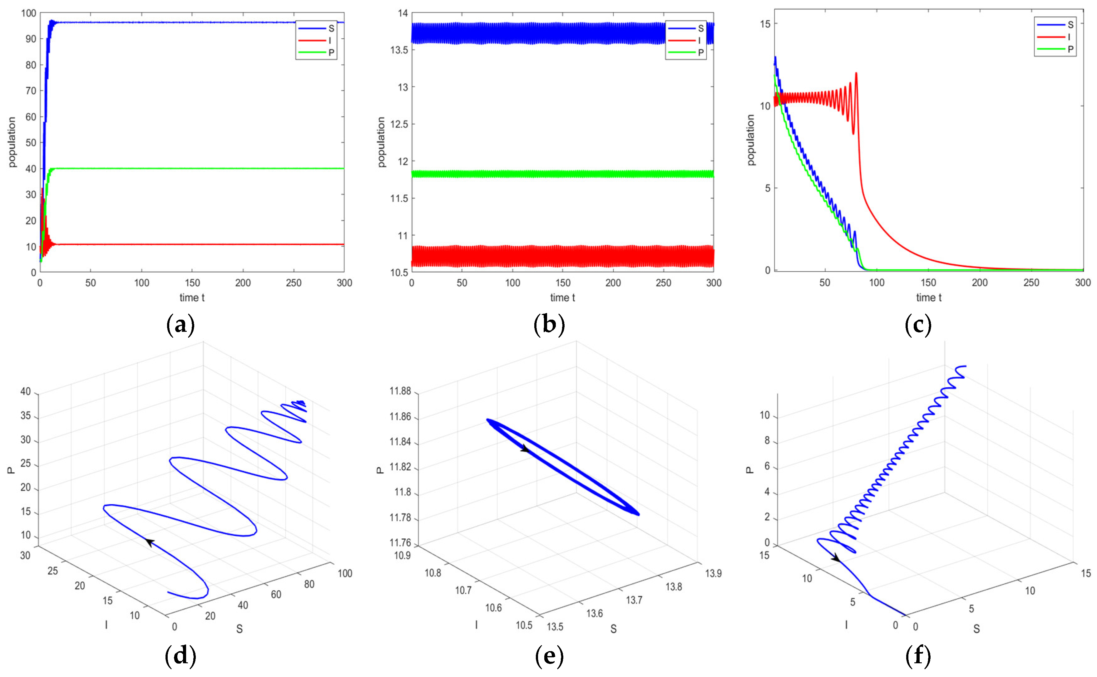
Figure 2 is based on the premise that the prey does not experience a weak Allee effect and studies the infection rate of the disease affecting the coexistence of species. Figure 2a,d show that when the prey is neither affected by the weak Allee effect nor infected by the disease, the predator is extinct due to the lack of food source, and the system finally only has susceptible prey. Figure 2b,c,e,f indicate that when the prey is not affected by the weak Allee effect, the infection intensity of the prey gradually increases. It is shown that a lower infection level can maintain the coexistence of multiple species, whereas a higher infection level induces periodic oscillations in the infected prey population.
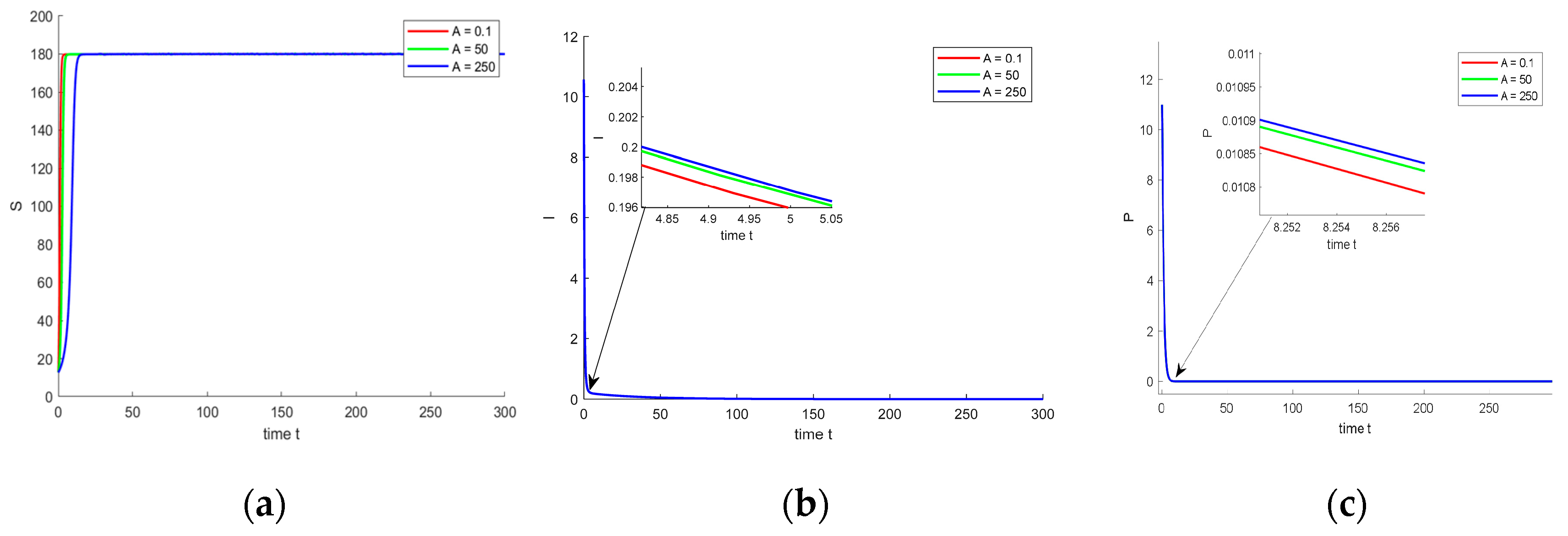
Figure 3 assumes that the prey population is not affected by disease. The effects of different intensities of the Allee effect on the coexistence state of the population are simulated. The results show that if the system is not affected by the disease, the population will never coexist.
Figure 4 shows that when A is used as the bifurcation parameter and β is controlled within a suitable range, the influence of the Allee effect on the dynamic behavior of species in the system is explored. Figure 4 clearly reveals that when the A value is low, the system remains stable. However, with the increase in the A value, the number of susceptible prey and predators gradually decreases, while the number of infected preys remains constant. When the A value reaches a specific threshold, the system oscillates. If the A value continues to increase, the system will eventually become extinct. Figure 5 is a further detailed explanation of Figure 4. The time series and phase diagrams of the critical value of Hopf bifurcation and the specific A values on both sides are drawn, respectively, to further clarify the dynamic change behavior of species.
Similarly, Figure 6 and Figure 7 simulate the change in β by controlling A in the appropriate range. The results show that with the increase in the β value, the number of populations gradually decreases, and there is a small oscillation in a specific interval, which eventually leads to the extinction of the system.
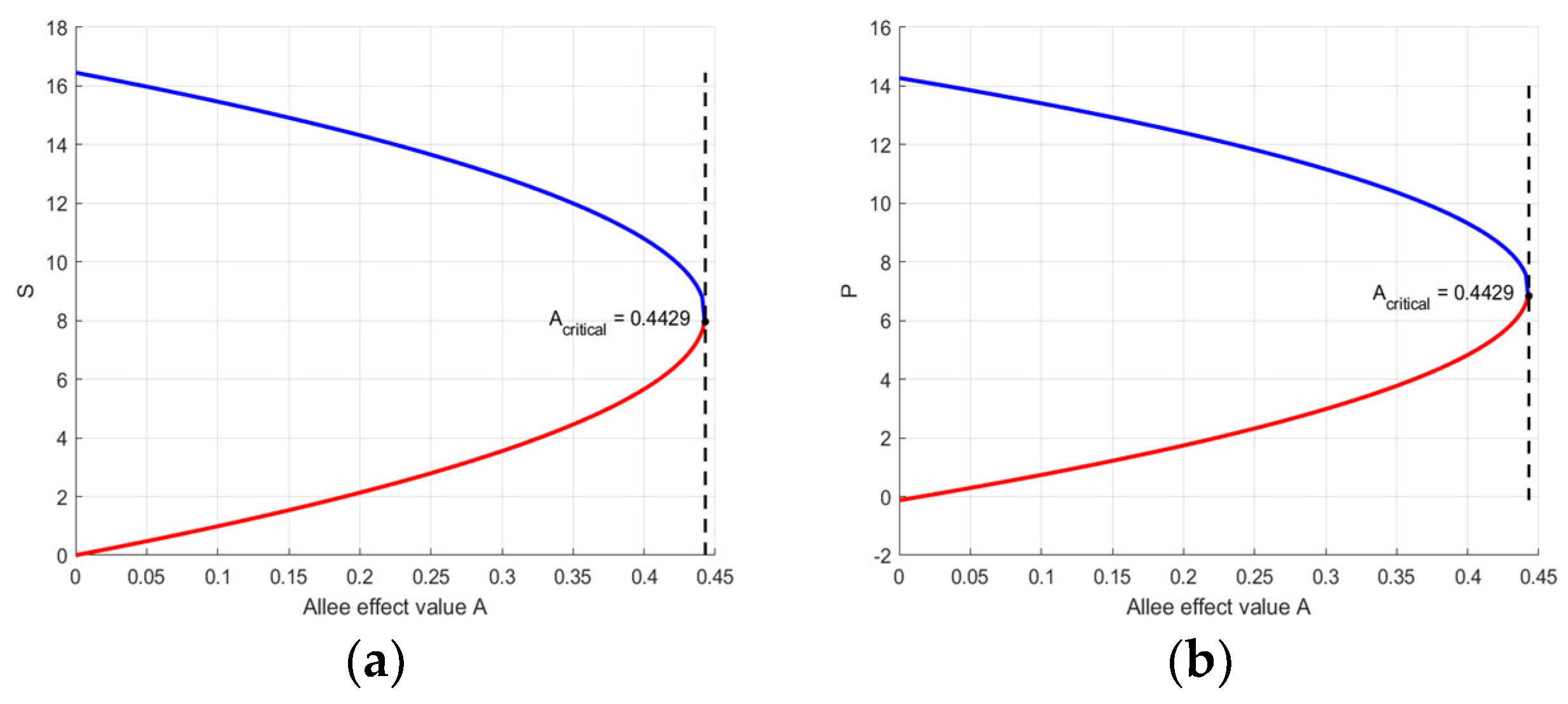
Figure 8 shows the saddle-node bifurcation of the coexistence equilibrium. When the value of parameter A is small, the model has two coexistence equilibrium points. As the parameter A increases to the critical value, these two equilibrium points gradually approach and eventually merge into a degenerate equilibrium point. When the parameter A continues to increase beyond the critical value, the degenerate equilibrium point disappears. The results show that the increase in Allee effect intensity may lead to population collapse. The mechanism is that under the condition of low population density, the mating probability between individuals is significantly reduced, which leads to the continuous decline in the population reproductive success rate. This positive feedback mechanism will aggravate the decline in the population and eventually lead to the population entering the irreversible extinction threshold range. Figure 9 shows the final trajectories of each equilibrium point under different initial states.

5. Conclusions

Eco-epidemiology is an interdisciplinary field in which various models have been developed to investigate the dynamics of disease transmission in populations. In model (1), the positivity and boundedness of solutions are analyzed. The local stability of feasible equilibria is also investigated. By taking the Allee effect parameter A and the disease transmission rate β as key control parameters, several types of bifurcations are identified, including transcritical bifurcation, saddle-node bifurcation, and Hopf bifurcation.
The Allee effect helps to understand the eco-epidemiological problems in the real world and plays an important role in maintaining system stability. It is observed that the Allee effect controls the stability of the system. The Allee effect can alter the stability of the equilibrium point, changing it from stable to unstable. Specifically, when parameter A is below the critical value of 0.312, the positive equilibrium point is stable; however, when A exceeds this critical value, it becomes unstable. Figure 4 and Figure 5 show how the weak Allee effect affects the dynamic process of species coexistence in an all-round way. In the case of controlling the incidence of disease in a suitable range, the influence of weak Allee effect parameter changes on species coexistence are analyzed. The results show that the increase in weak Allee effect parameters will reduce the size of predator and prey populations, and too high parameter values may even lead to population extinction.
The disease transmission rate β is also a crucial parameter that needs to be studied. The dynamical behavior of model (1) can be altered by this parameter. For lower values of infection rate, the system is stable. For a greater infection rate, the system performs a Hopf bifurcation, and periodic oscillations occur at about β = 0.209 .
Figure 6 and Figure 7 further illustrate the influence of different disease transmission rates on the coexistence of species in the system when the prey is affected by the Allee effect. The results show that the increase in disease transmission rate parameters will reduce the population size of predators and preys, and too high parameter values will lead to population extinction. In order to realize the coexistence of species in the system, it is necessary to control the intensity of disease transmission in the population and regulate the population size in a timely manner; otherwise the system may collapse.
This study is analyzed at only the theoretical level. However, in real ecological communities, population relationships may be more complex. Therefore, it would be interesting to consider more complex disease transmission mechanisms to enrich our model. Future research can further explore all these issues.

Author Contributions

Conceptualization, H.L. and Y.D.; methodology, H.L. and Y.D.; software, Y.D.; validation, H.L., Y.D., J.Y., G.M. and Y.W.; formal analysis, H.L., Y.D. and Y.W.; writing—original draft preparation, H.L. and Y.D.; writing—review and editing, H.L., Y.D., G.M. and Y.W.; visualization, H.L., Y.W. and Y.D.; supervision, H.L.; project administration, H.L.; funding acquisition, H.L. All authors have read and agreed to the published version of the manuscript.

Funding

This work was supported by the Gansu Provincial Education Department’s Graduate Student “Innovation Star” Project (2025CXZX-249, 2025CXZX-237), the Fundamental Research Funds for the Central Universities (31920240117; 31920250031), and the Innovation Team of Ecosystem Restoration Modeling Theory and Application of Northwest Minzu University (10017632).

Data Availability Statement

Data are contained within the article.

Conflicts of Interest

The authors declare no conflicts of interest.

Appendix A

The Jacobin matrix can be expressed as
J ( E ) = 2 r S K 3 r S 2 2 r S I K ( S + A ) r S 2 K r S 3 r S 2 I K ( S + A ) 2 β I r S 2 K ( S + A ) β S 0 β I β S c P d c I 0 e c P e c I m .
For the equilibrium E 0 , the Jacobian matrix is
J ( E 0 ) = 0 0 0 0 d 0 0 0 m .
For the equilibrium E 1 , the Jacobian matrix is
J ( E 1 ) = r K ( K + A ) r K ( K + A ) β K 0 0 β K d 0 0 0 m .
For the equilibrium E 2 , the Jacobian matrix is
J ( E 2 ) = r S ¯ 3 2 r A S ¯ 2 + ( r K A r I ¯ A ) S ¯ K ( S ¯ + A ) 2 r S ¯ 2 K ( S ¯ + A ) d 0 β I ¯ 0 c I ¯ 0 0 e c I ¯ m ,
where C 11 = r S ¯ 3 2 r A S ¯ 2 + ( r K A r I ¯ A ) S ¯ K ( S ¯ + A ) 2 , C 21 = β I ¯ , and C 12 = r S ¯ 2 K ( S ¯ + A ) d .
Let E S , I , P be any coexistence equilibrium point of the model (1). For the coexistence equilibrium E , the Jacobian matrix is
J ( E ) = c 11 c 12 0 c 21 0 c 23 0 c 32 0 ,
and we have
c 11 = r S 3 2 r A S 2 + ( r K A r I A ) S K ( S + A ) 2 , c 12 = [ r S 2 K ( S + A ) + β S ] < 0 , c 21 = β m e c > 0 , c 23 = m e < 0 , c 32 = e c P > 0 .

References

  1. Li, C. Protecting Endangered Animal Species. Animals 2024, 14, 2644. [Google Scholar] [CrossRef]
  2. Lotka, A.J. Elements of Physical Biology; Williams & Wilkins: Baltimore, MD, USA, 1925. [Google Scholar]
  3. Lotka, A.J. Fluctuations in the abundance of a species considered mathematically. Nature 1927, 119, 12. [Google Scholar] [CrossRef]
  4. Hadeler, K.P.; Freedman, H.I. Predator–prey population with parasite infection. J. Math. Biol. 1989, 27, 609–631. [Google Scholar] [CrossRef] [PubMed]
  5. Venturino, E. Epidemics in predator-prey models: Disease in the predators. Math. Med. Biol. 2002, 19, 185–205. [Google Scholar] [CrossRef]
  6. May, R.M.; Anderson, R.M. Population biology of infectious diseases: Part II. Nature 1979, 280, 455–461. [Google Scholar] [CrossRef] [PubMed]
  7. Allee, W.C. Animal Aggregations: A Study in General Sociology; University of Chicago Press: Chicago, IL, USA, 1931. [Google Scholar]
  8. Wei, C.; Chen, L. Periodic solution and heteroclinic bifurcation in a predator–prey system with Allee effect and impulsive harvesting. Nonlinear Dyn. 2014, 76, 1109–1117. [Google Scholar] [CrossRef]
  9. Biswas, S.; Sasmal, S.K.; Samanta, S.; Saifuddin, M.; Pal, N.; Chattopadhyay, J. Optimal harvesting and complex dynamics in a delayed eco-epidemiological model with weak Allee effects. Nonlinear Dyn. 2017, 87, 1553–1573. [Google Scholar] [CrossRef]
  10. Samanta, S.; Sen, P. Multistability and Chaos in the Eco-epidemiological System with Allee Effect. Differ. Equ. Dyn. Syst. 2024, 33, 1–24. [Google Scholar] [CrossRef]
  11. Shaikh, A.A.; Das, H. An eco-epidemic predator–prey model with Allee effect in prey. Int. J. Bifurc. Chaos 2020, 30, 2050194. [Google Scholar] [CrossRef]
  12. Ye, Y.; Liu, H.; Wei, Y.M.; Ma, M.; Zhang, K. Dynamic study of a predator-prey model with weak Allee effect and delay. Adv. Math. Phys. 2019, 2019, 7296461. [Google Scholar] [CrossRef]
  13. Li, D.; Liu, H.; Zhang, H.; Ma, M.; Ye, Y.; Wei, Y.M. Bifurcation Analysis in a Predator-Prey Model with an Allee Effect and a Delayed Mechanism. Acta Math. Sci. 2023, 43, 1415–1438. [Google Scholar] [CrossRef]
  14. Celik, C.; Duman, O. Allee effect in a discrete-time predator–prey system. Chaos Solitons Fractals 2009, 40, 1956–1962. [Google Scholar] [CrossRef]
  15. Javaid, Y.; Jawad, S.; Ahmed, R.; Ali, A.H.; Rashwani, B. Dynamic complexity of a discretized predator-prey system with Allee effect and herd behaviour. Appl. Math. Sci. Eng. 2024, 32, 2420953. [Google Scholar] [CrossRef]
  16. Liu, Y.; Zhang, Z.; Li, Z. The Impact of Allee Effect on a Leslie–Gower Predator–Prey Model with Hunting Cooperation. Qual. Theory Dyn. Syst. 2024, 23, 88. [Google Scholar] [CrossRef]
  17. Din, Q. Controlling chaos in a discrete-time prey-predator model with Allee effects. Int. J. Dyn. Control 2018, 6, 858–872. [Google Scholar] [CrossRef]
  18. Berec, L.; Angulo, E.; Courchamp, F. Multiple Allee effects and population management. Trends Ecol. Evol. 2007, 22, 185–191. [Google Scholar] [CrossRef]
  19. Møller, A.P.; Legendre, S. Allee effect, sexual selection and demographic stochasticity. Oikos 2001, 92, 27–34. [Google Scholar] [CrossRef]
  20. Courchamp, F.; Macdonald, D.W. Crucial importance of pack size in the African wild dog Lycaon pictus. In Animal Conservation Forum; Cambridge University Press: Cambridge, IL, USA, 2001; Volume 4, pp. 169–174. [Google Scholar]
  21. Avilés, L.; Tufino, P. Colony size and individual fitness in the social spider Anelosimus eximius. Am. Nat. 1998, 152, 403–418. [Google Scholar] [CrossRef]
  22. Mooring, M.S.; Fitzpatrick, T.A.; Nishihira, T.T.; Reisig, D.D. Vigilance, predation risk, and the Allee effect in desert bighorn sheep. J. Wildl. Manag. 2004, 68, 519–532. [Google Scholar] [CrossRef]
  23. Courchamp, F.; Berec, L.; Gascoigne, J. Allee Effects in Ecology and Conservation; OUP Oxford: Oxford, UK, 2008. [Google Scholar]
  24. Gascoigne, J.; Lipcius, R.N. Allee effects in marine systems. Mar. Ecol. Prog. Ser. 2004, 269, 49–59. [Google Scholar] [CrossRef]
  25. Berec, L. Mate search and mate-finding Allee effect: On modeling mating in sex-structured population models. Theor. Ecol. 2018, 11, 225–244. [Google Scholar] [CrossRef]
  26. Wang, L.; Qiu, Z.; Feng, T.; Kang, Y. An eco-epidemiological model with social predation subject to a component Allee effect. Appl. Math. Model. 2022, 101, 111–131. [Google Scholar] [CrossRef]
  27. Burrows, R.; Hofer, H.; East, M.L. Population dynamics, intervention and survival in African wild dogs (Lycaon pictus). Proc. R. Soc. Lond. Ser. B Biol. Sci. 1995, 262, 235–245. [Google Scholar]
  28. Courchamp, F.; Clutton-Brock, T.; Grenfell, B. Multipack dynamics and the Allee effect in the African wild dog, Lycaon pictus. In Animal Conservation Forum; Cambridge University Press: Cambridge, IL, USA, 2000; Volume 3, pp. 277–285. [Google Scholar]
  29. Gabera, T.; Widowati, R.H. The impact of ecological mechanisms on stability in an eco-epidemiological model: Allee effect and prey refuge. Comput. Res. Model. 2025, 17, 139–169. [Google Scholar]
  30. Angulo, E.; Roemer, G.W.; Berec, L.; Gascoigne, J.; Courchamp, F. Double Allee effects and extinction in the island fox. Conserv. Biol. 2007, 21, 1082–1091. [Google Scholar] [CrossRef]
  31. Clifford, D.L.; Mazet, J.A.K.; Dubovi, E.J.; Garcelon, D.K.; Coonan, T.J.; Conrad, P.A.; Munson, L. Pathogen exposure in endangered island fox (Urocyon littoralis) populations: Implications for conservation management. Biol. Conserv. 2006, 131, 230–243. [Google Scholar] [CrossRef]
  32. Saifuddin, M.; Biswas, S.; Samanta, S.; Sarkar, S.; Chattopadhyay, J. Complex dynamics of an eco-epidemiological model with different competition coefficients and weak Allee in the predator. Chaos Solitons Fractals 2016, 91, 270–285. [Google Scholar] [CrossRef]
  33. Sasmal, S.K. Population dynamics with multiple Allee effects induced by fear factors—A mathematical study on prey-predator interactions. Appl. Math. Model. 2018, 64, 1–14. [Google Scholar] [CrossRef]
  34. Kumar, B.; Sinha, R.K. Dynamics of an eco-epidemic model with Allee effect in prey and disease in predator. Comput. Math. Biophys. 2023, 11, 20230108. [Google Scholar] [CrossRef]
  35. Ghosh, S.; Mukherjee, C.; Panigrahi, G.; Biswas, S. Dynamics of alternative food and allee effect in an eco-epidemiological system with disease in predator. Nonlinear Stud. 2023, 30, 1025. [Google Scholar]
  36. Nath, B.; Kumar, V.; Kumari, N.; Pada Das, K.; Maiti, S. A study of chaos and its possible control in an eco-epidemiological model with alternative food source in predator and weak allee effect in prey species. Nonlinear Stud. 2020, 27, 725. [Google Scholar]
  37. Diekmann, O.; Heesterbeek, J.A.P.; Metz, J.A.J. On the definition and the computation of the basic reproduction ratio R0 in models for infectious diseases in heterogeneous populations. J. Math. Biol. 1990, 28, 365–382. [Google Scholar] [CrossRef] [PubMed]
  38. Van den Driessche, P.; Watmough, J. Reproduction numbers and sub-threshold endemic equilibria for compartmental models of disease transmission. Math. Biosci. 2002, 180, 29–48. [Google Scholar] [CrossRef] [PubMed]
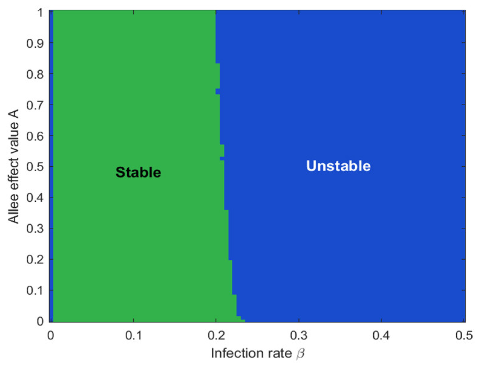
Figure 1. Two parameter bifurcation diagrams in the βA plane. The figure shows a two-parameter bifurcation diagram in the βA plane, describing the stability of the coexistence equilibrium of model (1) as the parameters β and A change. The coexistence equilibrium is unstable in the blue region and stable in the green region.
Axioms 14 00531 g001
Figure 2. The figures show the time series and phase diagrams of susceptible prey, infected prey, and the predator in the following cases: (a,d) A = β = 0 ; (b,e) A = 0 , β = 0.1 ; and (c,f) A = 0 , β = 0.9 , respectively. Other parameters are given in Equation (6).
Axioms 14 00531 g002
Figure 3. Under the premise of disease infection rate β = 0 , the time series diagrams of susceptible prey (a), infected prey (b), and the predator (c) under different A values are drawn. Other parameters are given in Equation (6).
Axioms 14 00531 g003
Figure 4. When β = 0.21 , the Hopf bifurcation diagram of the susceptible prey (a), infected prey (b), and the predator (c) population of model (1) with respect to A is shown. Other parameters are given in Equation (6).
Axioms 14 00531 g004
Figure 5. The time series diagram and phase diagram of Figure 5 at the critical point of Hopf bifurcation when (a,d) A = 0.001 , (b,e) A = 0.312 , and (c,f) A = 0.34 are drawn.
Axioms 14 00531 g005
Figure 6. When A = 0.312 , the Hopf bifurcation diagram of the susceptible prey (a), infected prey (b), and predator (c) population of model (1) with respect to β is shown. Other parameters are given in Equation (6).
Axioms 14 00531 g006
Figure 7. The time series diagram and phase diagram of Figure 6 at the critical point of Hopf bifurcation when (a,d) β = 0.1 , (b,e) β = 0.209 , and (c,f) β = 0.22 are drawn.
Axioms 14 00531 g007
Figure 8. (a) The saddle-node bifurcation diagram of S population; (b) The saddle-node bifurcation diagram of P population.
Axioms 14 00531 g008
Figure 9. The trajectory diagram of the equilibrium points under different initial conditions. The parameters (a K = 180 , A = 0.31 , and β = 0.21 ; (b) K = 180 , A = 0.31 , and β = 0.000015 ; (c) K = 10 , A = 0.001 , and β = 0.01 , and other parameters are given in Equation (6).
Axioms 14 00531 g009
Disclaimer/Publisher’s Note: The statements, opinions and data contained in all publications are solely those of the individual author(s) and contributor(s) and not of MDPI and/or the editor(s). MDPI and/or the editor(s) disclaim responsibility for any injury to people or property resulting from any ideas, methods, instructions or products referred to in the content.