1. Introduction
Network reliability is a popular research topic in the fields of network performance analysis, combinatorial mathematics, and graph theory. These studies usually explore the network by transforming it into its topology, which is a graph (where the nodes in the network correspond to the vertices in the graph and the links in the network correspond to the edges between the corresponding vertices in the graph). Therefore, in this paper, we will not make a clear distinction between networks and graphs.
Currently, research on reliability under edge failure but vertex reliability in networks has focused on the following areas. Firstly, from the number of key vertices in the network, studies have been differentiated into two cases:
k-terminal networks (where
) [
1,
2] and all-terminal networks (i.e.,
) [
3,
4,
5]. Secondly, in terms of research direction, reliability research is split into two primary areas: reliability analysis [
1,
5,
6,
7] and reliability design [
8,
9,
10,
11,
12]. Reliability analysis focuses on calculating the probability that a network will be able to work under conditions of edge failure, which is usually quantified by a reliability polynomial, while reliability design aims to construct a network structure that maximizes the value of this reliability polynomial.
Reliability studies have focused mainly on the field of analysis and design of all-terminal networks [
1,
3,
4,
6,
8], while relatively few investigations on
k-terminal reliability have focused on developing efficient algorithms for computing
k-terminal reliability polynomials [
1,
7,
13]. However, in recent years, research on
k-terminal reliability design has shown a gradual increase [
2,
9,
10,
11,
12]. In 2018, Bertrand et al. [
9] studied the existence of a uniformly optimal structure under edge failure for two-terminal graphs when
and when
. In other words, they explored whether there exists a structure, regardless of the value of the edge failure probability, which can maximize reliability of two-terminal graphs. In addition, they characterize several locally most reliable two-terminal graphs that are maximized when the probability of edge failure approaches 0 or 1. In 2021, Xie et al. [
10] analyzed the properties of two types of locally most reliable two-terminal graphs, and accordingly determined that there exists no uniformly most reliable two-terminal graph when
, which further enhances the theoretical framework of the consistent optimality problem for two-terminal graphs. Building on this foundation, in 2024, Gong et al. [
2] inscribed the locally most reliable two-terminal graph for satisfying
and
m not close to
under the condition that the probability of edge failure tends to 1.
Based on the research results on the optimality of two-terminal networks, Xie et al. [
11,
12], in 2021, explored the reliability problem of three-terminal networks by inscribing locally most reliable three-terminal graphs with edge numbers
m in
and
.
However, most of the research focuses on constructing locally most reliable graphs. When many edges in the graph are failed, it is not clear which edge is repaired priorly to reduce the loss for network failure at the fastest speed. In real life, we need to study the structure of the locally most reliable graph, while also exploring a way of designing a structure with higher reliability. According to actual demand, we build a relatively reliable network under the condition of resource constraints and realize the balance between resource saving and demand satisfaction. Additionally, we provide a theoretical basis for quickly repairing critical edges if the network experiences failure.
In this paper, by comparing the reliability polynomial coefficients of three-terminal graphs step by step, we obtain three comparative judgment criteria for reliability under the condition of high edge failure probability. These criteria provide a scheme to prioritize edge connections and construct a more reliable structure. Meanwhile, according to the judgment criteria, we characterize locally most reliable three-terminal graphs in the range
and
with edge failure probabilities close to 1. The locally most reliable three-terminal graphs obtained by this method are consistent with the results in [
11,
12], thereby verifying the validity and accuracy of our method. Furthermore, the study of locally optimal structures for other ranges have been limited to six special classes of graphs, which significantly reduces the complexity. Finally, we propose a search method that identifies the locally most reliable three-terminal graphs or locally more reliable three-terminal graphs based on the judgment criteria.
This paper is organized as follows. In
Section 2, some basic definitions and related notations are introduced. In
Section 3, three local reliability comparison criteria are stated and several locally most reliable three-terminal graphs by these criteria are characterized. In
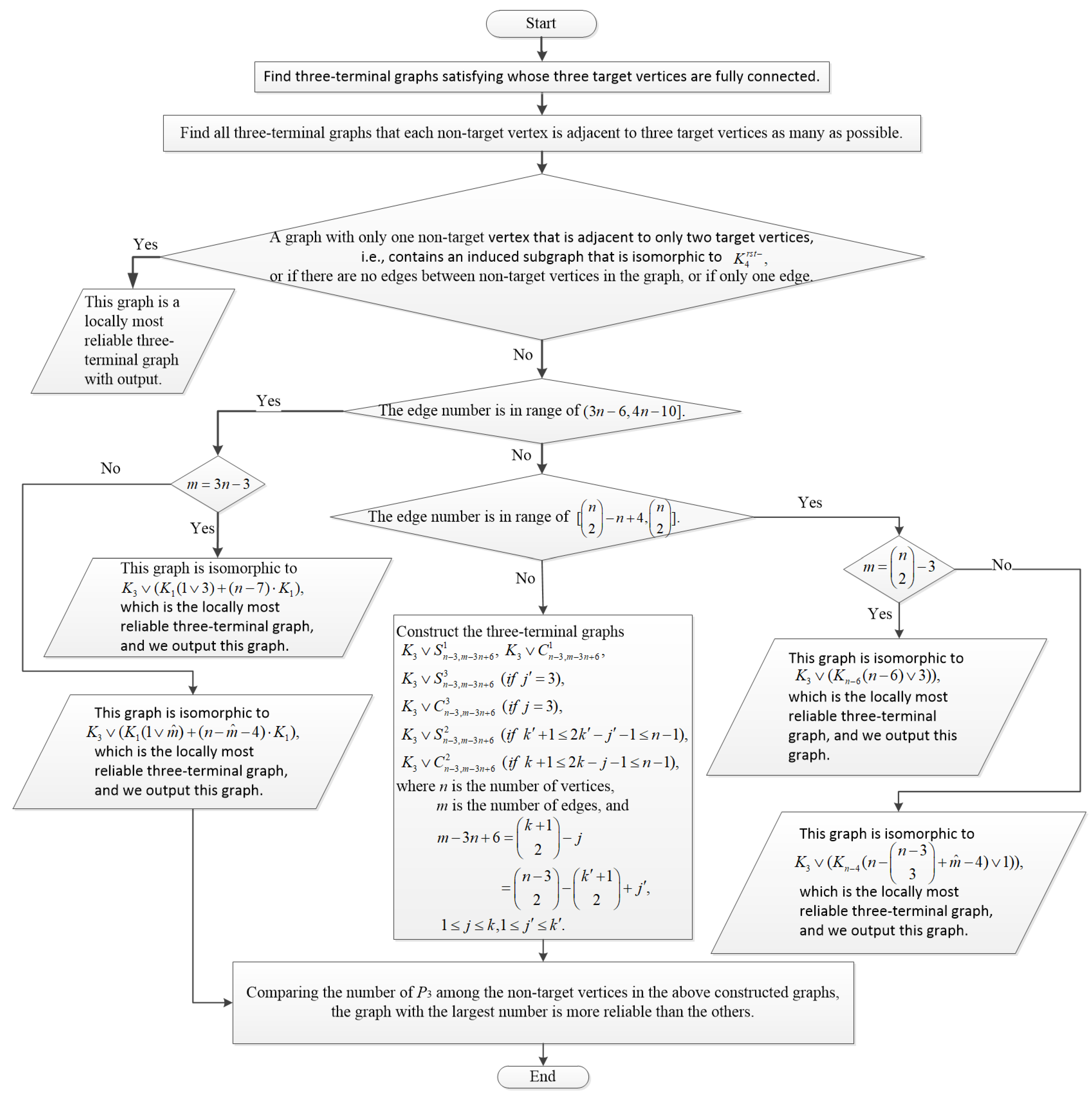
Section 4, a flowchart is given to find the locally optimal structures by the criteria.
Section 5 summarizes the paper and puts forward some interesting problems to be solved.
2. Basic Concepts and Notations
This section introduces some symbolic terms and basic concepts. For those not mentioned, see [
14]. The graph without loops or parallel edges is the simple graph. In this paper, we study only simple graphs. For graphs
G and
H, if there are bijections
:
and
:
such that
if and only if
, then
G and
H are isomorphic, written as
. Use
to denote the graph with vertex set
and edge set
. Let
denote the number of the induced subgraphs of
G isomorphic to
H. Let
denote the number of subgraphs of
G that are isomorphic to
H. Using
denotes the path in the graph with
i vertices and
edges.
A simple graph is a three-terminal graph if the vertex set has three specified key vertices (target vertices) and t, and an all-terminal graph if all vertices are key vertices. Denote by the set of all three-terminal graphs on n vertices and m edges. Denote by the set of all all-terminal graphs on n vertices and m edges. The reliability (or the reliability polynomial) of three-terminal graph G, denoted by , is the probability that the three specified target vertices in graph remains connected when its edges fail independently with probability q.
An
-subgraph is a subgraph of
G in which
are connected. This
-subgraph is minimal if it is not an
-subgraph after deleting any of its edges, otherwise it is a non-minimal
-subgraph. If an
-subgraph has
i edges, it is denoted as
. Since
and
do not exist, the reliability polynomial of three-terminal graph
can be written as
where
or simply
is the number of
-subgraph
in graph
G.
Definition 1 ([
11]).
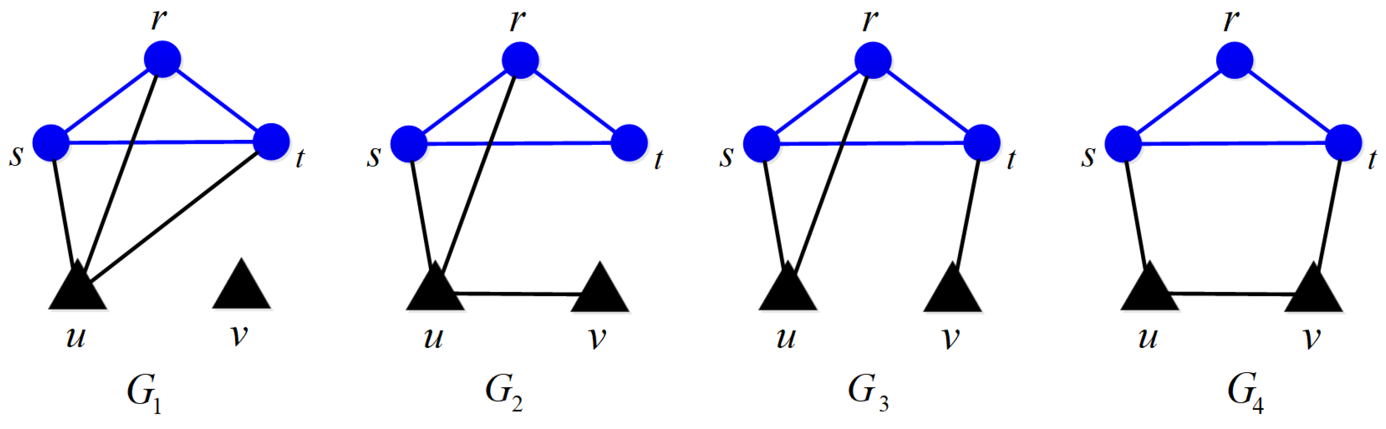
A graph G is the locally most reliable graph in if for and . Example 1. The following four graphs given in Figure 1 all show the topology of a regional power supply network with five vertices and six edges. The blue circular vertices represent three key substations (target vertices): r (main supply to the urban core), s (main supply to the industrial area), and t (main supply to the outskirts of the city and important public utilities). The black triangular vertices represent auxiliary power supply facilities (non-target vertices): small-scale power generation stations and backup power facilities. The target vertices are responsible for converting high-voltage electrical energy into low-voltage electrical energy suitable for use in urban or industrial areas and distributing it to each user end. The non-target vertices can provide additional power support to the target vertices or serve as backup power sources. If the edge (supply line) failure probability is q, then for , -subgraphs ( and ) with zero edges and with one edge do not exist, so . The -subgraphs with two edges are , , , so . The -subgraphs with three edges are , , , , , , , , , , , , , , , , , so . The -subgraphs with four edges are , , , , , , , , , , , , , , , so . The -subgraphs with five edges are , , , , , , so . The -subgraph with six edges is , so .
Therefore, the reliable polynomial of
is
. Similarly, the reliable polynomials of
,
, and
are
,
, and
, respectively. Obviously,
for
q close to 1. In fact, it has been proved in [
11] that
is the most reliable graph in
. So, the critical packet certified regional power supply network maintains the stable transmission and distribution of electric energy, and this network can be constructed according to the structure of
. However, when more than one edge of the network fails, in order to reduce the loss as soon as possible, it is necessary to choose the line that is prioritized for repair, so the characterization of a more reliable network is necessary, and the next sections will give the related research.
3. Judgment Criteria of the Local Reliability Comparison with High Edge Failure Probability
In this section, we focus on the characterization of more reliable graphs by giving three locally more reliable comparison judgment theorems. Then, we construct several locally most reliable three-terminal graphs for
q close to 1. We compare the results with existing literature results to further verify the validity and accuracy of the judgment theorems. In general, the calculation of the three-terminal reliability polynomial of the graph is NP-hard [
15]. Therefore, we study the reliability of graphs by the following lemma.
Lemma 1. Let the three-terminal reliability polynomials of G and H in be and , respectively.
Suppose there exists a positive integer k such that and for , then holds when .
Proof. Since
, it is clear that
Since
,
For and , it is easy to see that . So, if , then as ; that is, . □
From Lemma 1, we can derive the first round of the local reliability comparison criterion for a three-terminal graph with high edge failure probability. It is referred to as the First Judgment Criterion ().
For a graph , let be the number of edges among the target vertices and t in G; that is, .
Theorem 1 (First Judgment Criterion ()). Let , if , then for , , which means that G is locally more reliable than H for .
Proof. The number of -subgraph with two edges of G and H can be expressed as and .
If , then . By Lemma 1, we see that as q approaches 1, which indicates that G is more reliable than H for . □
According to the First Judgment Criterion (), in order to find the locally most reliable three-terminal graph as q approaches 1, one must first identify the class of all three-terminal graphs in that contain the maximum number of edges in the triangle formed by three target vertices. For convenience, this class is denoted as .
Obviously, there are many graphs in . To search the locally most reliable three-terminal graph for , we further construct a second round of the local reliability comparison criterion in .
The three-terminal complete graph with n vertices, denoted by , is a simple graph that has 3 target vertices and non-target vertices, where any two vertices are adjacent. If an edge connecting one target vertex and one non-target vertex is deleted in the graph , the resulting graph is denoted by .
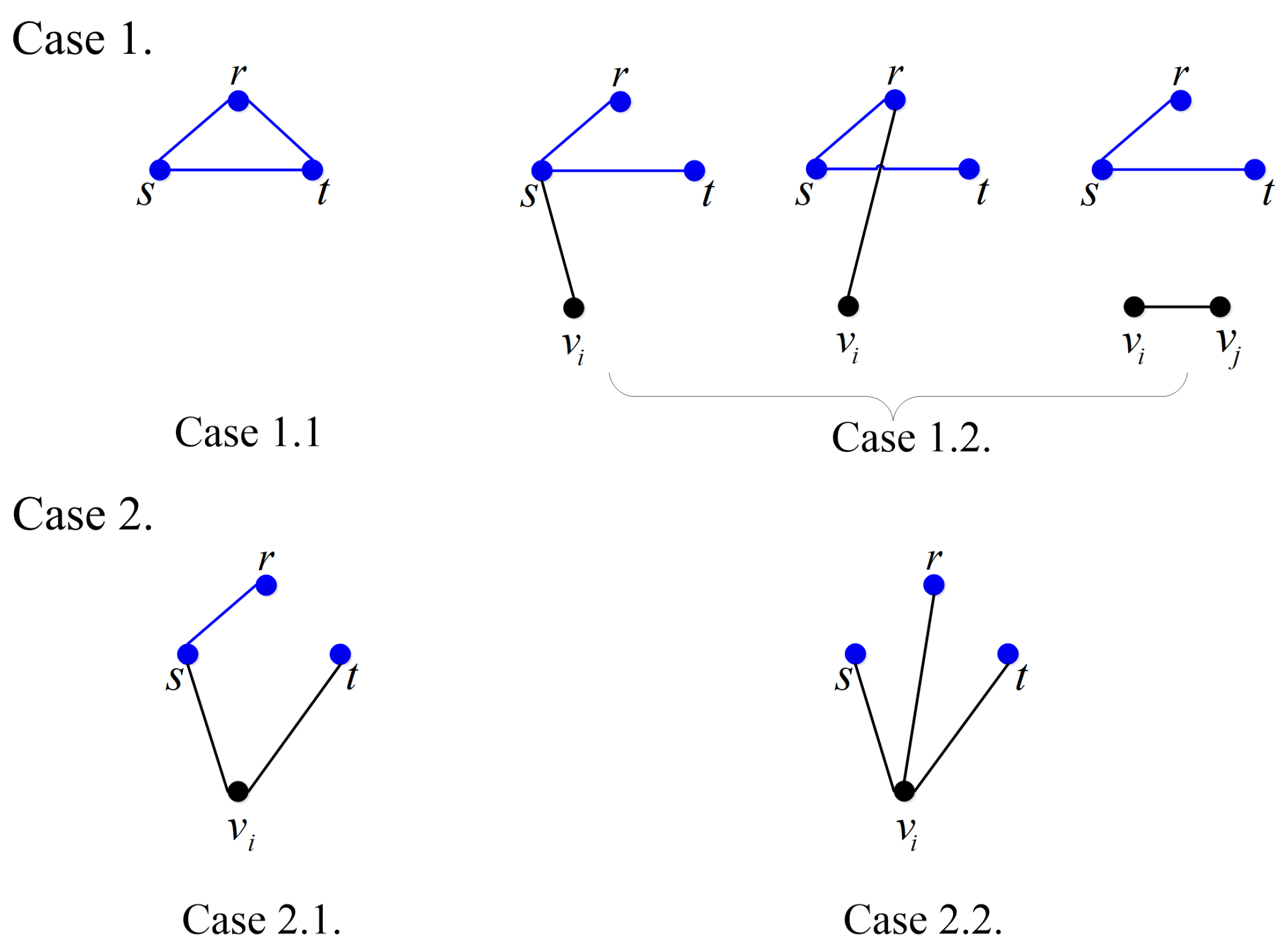
Theorem 2 (Second Judgment Criterion ()). Let and . If , then , which means that G is locally more reliable than H for .
Proof. Since , the triangle is contained in G and H, which means that . Thus, .
Then, by Lemma 1, we need to compare the values of
and
. Now, we consider the
-subgraphs
in
G and
H, as shown in
Figure 2.
- Case 1
is a non-minimal -subgraphs with three edges.
- Subcase 1.1
contains all the edges of the triangle , which means that . Obviously, the number of in this subcase is 1.
- Subcase 1.2
contains two edges of the triangle , which means that , where and . The number of in this subcase is .
- Case 2
is a minimal -subgraphs.
- Subcase 2.1
contains one edge of the triangle . Without loss of generality, assume that , where . The number of in this subcase is , which equals .
- Subcase 2.2
contains no edge of the triangle , which means that , where . The number of in this subcase is , which equals .
Combining the results of above cases, we have
Similarly, it can be obtained that .
Clearly, if , then .
Therefore, by Lemma 1, it follows that for , and the theorem holds. □
According to the Second Judgment Criterion (), to find the locally most reliable three-terminal graph as , it is necessary to identify the class of graphs within that maximizes the sum of two times the number of induced subgraphs isomorphic to and seven times the number of induced subgraphs isomorphic to . This class is denoted as .
Indeed, in a three-terminal graph G containing triangles , the number of induced subgraphs isomorphic to must be maximized in order to get the maximum value of . In other words, each non-target vertex is adjacent to three target vertices as many as possible, as seen in Theorem 3.
Theorem 3. Let , then , and Proof. Since , it follows that for any three-terminal graph H in . For convenience, let and . It is easy to see that . Otherwise, there must exist two non-target vertices and such that G contains two edges in , and two edges in . Without loss of generality, assume that these four edges are , , , and , then there must exist a graph () satisfying , . Thus, we have that is, , a contradiction.
Clearly, . Since , . Otherwise, for any graph in containing induced subgraphs , there is , a contradiction.
Moreover, when , . At this point, if or , then clearly, holds; if , then . When , , in this case .
In conclusion, we complete the proof. □
Theorem 3 determines the number of induced subgraphs
and induced subgraphs
of the locally most reliable three-terminal graph as
. Consequently, we can directly determine the locally optimal structure for
and
or
. Please refer to the following corollary, which is consistent with the results of Theorem 3.1 and Theorem 3.2 in [
11].
Corollary 1. Let G be the locally most reliable three-terminal graph in at , then
for and , ;
for and , .
However, when and , or when , the locally most reliable three-terminal graph () cannot be determined only based on the Second Judgment Criterion. Therefore, we begin to construct the third criterion for local reliability comparison among three-terminal graphs with high edge failure probability. This will be referred to as the Third Judgment Criterion ().
For , let . Obviously, , .
Theorem 4 (Third Judgment Criterion ()). Let , and satisfy the above establishment. If one of the following conditions holds when and , or , then as ; that is, G is locally more reliable than H when q approaches 1.
;
, but .
Proof. Since
,
. For
and
, or
, by Theorem 3, it is easy to see that
and
Thus, combined with the proof of Theorem 2, we obtain
By Lemma 1, in order to compare the reliability of G and H, we need to compare and . Consider the cases of in G and H.
- Case 1
is a non-minimal -subgraph with four edges.
- Subcase 1.1
The minimal -subgraph contained in has two edges, which means that , where . The number of in this subcase is .
- Subcase 1.2
The minimal -subgraph contained in has three edges, which means that or , where . The number of in this subcase is , which equals .
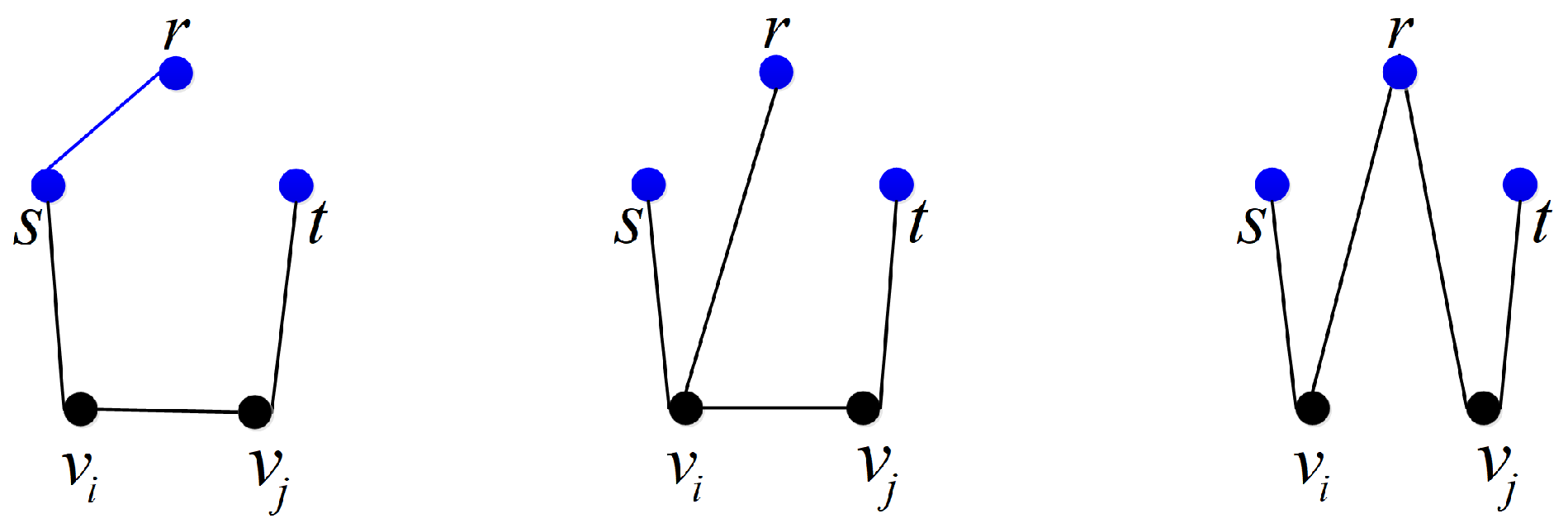
- Case 2
is a minimal
-subgraph, as shown in
Figure 3, which means that
,
or
, where
. The number of
in this case is
, which equals
.
Therefore,
- (1)
If , then ; that is . So, by Lemma 1, for .
- (2)
If , then . So, we need to further compare the values of and , and the -subgraph of a three-terminal graph has the following cases.
- Case 1
is a non-minimal -subgraph with five edges.
- Subcase 1.1
The minimal -subgraph contained in has two edges, which means that , , where . The number of in this subcase is , which equals .
- Subcase 1.2
The minimal -subgraph contained in has three edges, which means that or , , where , . The number of in this subcase is , which equals .
- Subcase 1.3
The minimal -subgraph contained in has four edges, which means that , , or ∉, or (, where , . The number of in this subcase is , which equals .
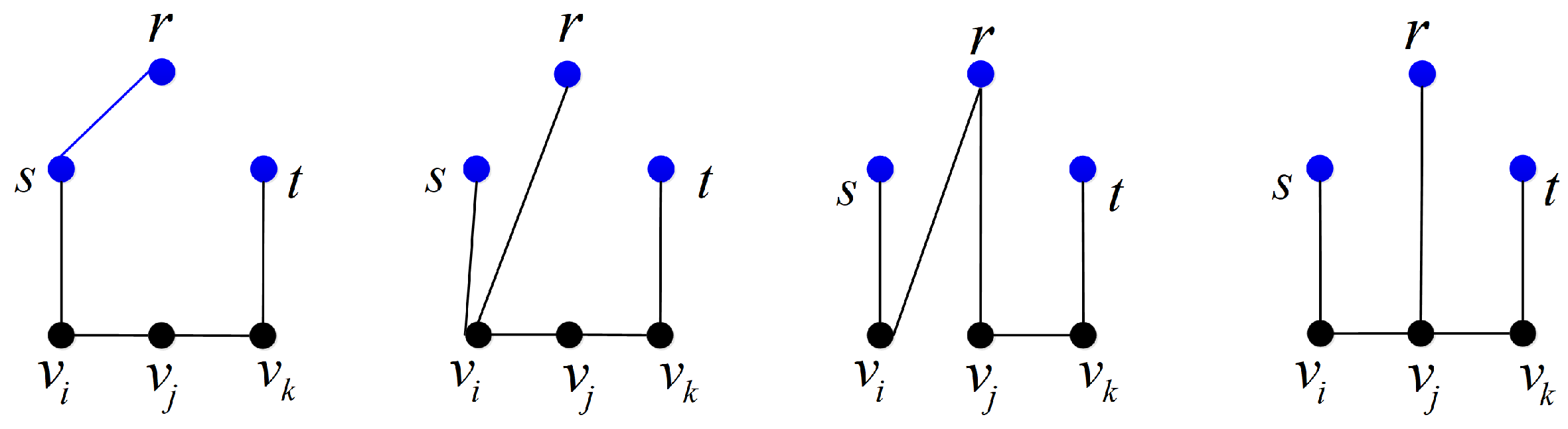
- Case 2
is a minimal
-subgraph, as shown in
Figure 4, which means that
,
,
or
, where
. The number of
in this case is
, which equals
.
It is easy to see that .
Clearly, if , then ; that is, . So, by Lemma 1, for .
In conclusion, we complete the proof. □
According to the Third Judgment Criterion (
), it is easy to see that for
and
, there is only one graph that satisfies the condition, and hence, it is the locally most reliable three-terminal graph (
), leading to the following corollary, which is consistent with Theorem 3.1 in [
11].
Corollary 2. Let and , if G is the locally most reliable three-terminal graph in for , then .
In addition, when , all non-target vertices in all graphs within are adjacent to three target vertices, and the number of subgraphs induced by these non-target vertices that contain is consistently . According to Lemma 1, to find the locally most reliable three-terminal graph for and , we must find the structure within such that the subgraph induced by non-target vertices with the maximum number of . This graph class is denoted as . In fact, finding can be translated into finding the all-terminal graph in with the maximum number of .
Up to now, numerous studies have focused on the problem of maximizing the number of
in
. In 1999, Byer [
16] characterized six types of graphs in
and proved that graphs with the most
belong to this set. In 2009, Ábrego et al. [
17] classified six types of graph divisions based on edge counts of graphs and established that the partition of graphs containing at most
in
must belong to one of these six classifications. Consequently, by combining and extending the relevant results in [
16,
17], we conclude that
is composed of several graphs from among these six types, as stated in Lemma 2.
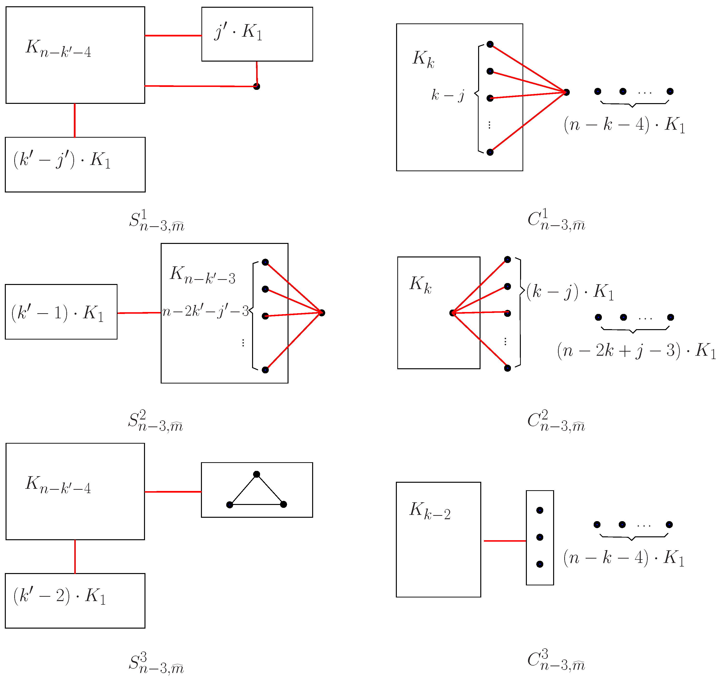
Lemma 2. Let , and be the unique integers satisfying the following condition,If H is a graph with the maximum number in , then H belongs to at least one of the following six classes. -Quasi-Star graph;
, where ;
, where ;
-Quasi-Complete graph;
, where ;
, where .
In particular,
- (1)
when ,
if, then or ;
if, then .
- (2)
when ,
if, then or ;
if, then .
Lemma 3. Let , and , if G is the locally most reliable three-terminal graph for , then , and must belong to , , which are shown as Figure 5. In particular,
- (1)
when ,
if, then or ;
if, then .
- (2)
when ,
if, then or ;
if, then .
Proof. Let G be the locally most reliable three-terminal graph for , then by Theorem 4, we have and .
Since has the maximum number in , then by Lemma 2, we see that belongs to .
In particular, if , then , and if , then . Therefore, by Lemma 2, the corresponding conclusion in this lemma holds.
In conclusion, we complete the proof. □
Lemma 3 gives locally most reliable three-terminal graphs for
and
, and the conclusions agree with the result of Theorem 3.7 in [
11] and the result of Theorem 1 in [
12], respectively.
Moreover, for
and
, Lemma 3 restricts the locally most reliable three-terminal graphs to two classes. Furthermore, in [
11],
is the locally most reliable three-terminal graphs for
and in [
12],
is the locally most reliable three-terminal graphs for
.


