Note on Iterations of Nonlinear Rational Functions

Abstract

This paper investigates a class of nonlinear rational difference equations with delayed terms, which often arise in various mathematical models. We analyze the iterative behavior of these rational functions and show how their iterations can be represented through second-order linear recurrence relations. By establishing a connection with generalized Balancing sequences, we derive explicit formulas that describe the system’s asymptotic behavior. Our main contribution is proving the existence of a unique globally asymptotically stable equilibrium point for all trajectories, regardless of initial conditions. We also provide analytical expressions for the solutions and support our findings with numerical examples. These results offer valuable insights into the dynamics of nonlinear rational systems and form a theoretical basis for further exploration in this area.

1. Introduction

The study of nonlinear rational difference equations has attracted considerable attention due to their intricate dynamic behaviors and frequent occurrence in applied mathematical models. Foundational studies have analyzed the global behavior and stability of rational systems [1,2]. Other works have explored periodicity, oscillations, and boundedness in various classes of nonlinear systems [3,4,5,6,7,8,9]. More recent studies have extended these results to higher-order and coupled systems, including those with variable or periodic coefficients [10,11,12,13,14]. These developments have emphasized the importance of analytical tools for understanding the long-term dynamics of such systems. In this paper, we investigate the iterative behavior of a specific class of nonlinear rational functions defined through a system of coupled recurrence relations. Building on earlier work, we extend the analysis of such systems by establishing a formal connection between their iterative dynamics and linear second-order difference equations.

Our focus centers on a general rational function of the form $f\left(y\right)={\displaystyle \frac{a+by}{c+dy}}$, with integer coefficients, and we explore the conditions under which its iterations can be represented in a closed rational form. This representation enables a deeper understanding of the convergence properties of the iterated sequences and reveals their asymptotic behavior through the lens of characteristic polynomials.

The class of nonlinear rational difference equations studied in this work appears frequently in diverse applied contexts, especially in engineering and control theory. For instance, such equations are commonly used in modeling feedback systems where the current state depends on past outputs in a rational form, including digital filters, population dynamics, and economic systems. In electrical engineering, rational difference equations can describe recursive filters used in signal processing, where stability and convergence of the output signal are of primary concern. Similarly, in control engineering, these equations model discrete-time control systems with nonlinear feedback components, particularly when the control law involves rational terms due to actuator saturation or nonlinear sensors.

The analysis of nonlinear rational difference equations has recently gained attention through advancements in numerical modeling [15], algebraic structures [16], and the theory of uncertain numbers [17], providing new insights into their iterative behavior.

The motivation for studying the nonlinear rational function stems from its widespread occurrence in mathematical models of real-world phenomena [18,19,20]. Such functions are known to exhibit rich and intricate dynamical behaviors, including oscillations, convergence to fixed points, and stability properties. Investigating these properties not only enhances the theoretical understanding of nonlinear difference equations, but also has potential applications in various scientific and engineering disciplines where such models naturally arise.

Several previous works have investigated systems of difference equations whose solutions are expressed in terms of generalizations of well-known sequences. Notably, researchers have extended classical sequences such as the Fibonacci [21,22,23], Padovan [24,25,26], Lucas sequences [27], and Pell sequence [28] to construct explicit solutions for various nonlinear and higher-order systems. These generalized sequences have proven to be effective tools in analyzing the dynamic behavior and asymptotic properties of such systems. Our work builds on this foundation by introducing a new generalized Balancing sequence tailored to rational difference equations.

A significant contribution of this work is the derivation of an explicit analytical relationship between the nonlinear system and a generalized form of the classical Balancing sequence. By introducing suitable transformations and exploiting the properties of associated bilinear difference equations, we demonstrate how nonlinear dynamics can be captured by linear recurrence relations.

Furthermore, we identify equilibrium points for the system and rigorously prove the global asymptotic stability of one of them, showing that all trajectories converge to a unique fixed point, regardless of initial conditions. Theoretical findings are substantiated with numerical simulations, which illustrate the convergence behavior and visualize the dynamics in phase space.

Compared to recent methods that primarily rely on numerical or approximate techniques to analyze difference equations, our approach offers explicit analytical solutions that accurately describe the system’s dynamics. The use of a generalized Balancing sequence provides a powerful alternative to other generalized sequences, such as Fibonacci and Padovan, in capturing convergence and stability behavior. This enhances the efficiency of the proposed method and opens new directions for studying more complex systems.

Through this comprehensive analysis, the paper contributes novel insights into the structure and behavior of nonlinear rational iterative systems and enhances the theoretical framework for understanding their long-term evolution. The authors in [29] proposed a solution to the open problem

$$x_{n+1}={\displaystyle \frac{1}{A-y_{n-k}}},y_{n+1}={\displaystyle \frac{1}{B-x_{n-k}}},n,k\in {\mathbb{N}}_0=\mathbb{N}\cup \left\{0\right\},$$

(1)

for $A,B\in \mathbb{R}$. Clearly, (1) provides

$$x_{n+1}={\displaystyle \frac{1}{A-y_{n-k}}}={\displaystyle \frac{1}{A-\frac{1}{B-x_{n-2k-1}}}}={\displaystyle \frac{B-x_{n-2k-1}}{AB-1-A{x}_{n-2k-1}}}.$$

(2)

Setting

$$u_n=x_{(2k+2)n},$$

we obtain

$$u_{n+1}={\displaystyle \frac{B-u_n}{AB-1-A{u}_n}}.$$

(3)

We consider a general case of (2) for a function

$$f\left(y\right)={\displaystyle \frac{a+by}{c+dy}},$$

(4)

for $a,b,c,d\in \mathbb{Z}$. We look for conditions that $f\left(y\right)$ has an iteration $y_{n+1}=f\left(y_n\right)$, $n\in {\mathbb{N}}_0$ of a form

$$y_n={\displaystyle \frac{r{p}^n+s{q}^n}{u{p}^n+v{q}^n}},$$

(5)

for suitable $r,s,u,v,p,q\in \mathbb{R}$, $p\ne q.$

The main objective of this paper is to explore the iterative dynamics of a class of nonlinear rational difference equations by establishing an explicit analytical framework that connects them with second-order linear recurrence relations. Our approach leads to the introduction of a generalized Balancing sequence that effectively describes the long-term behavior of the system.

In addition to these contributions, it is important to note that several existing methods have been developed to study difference equations with delays, such as the differential transform method (DTM) [30]. While DTM is valued for its simplicity and ability to handle delayed arguments, it generally provides only approximate solutions and may suffer from limited accuracy in long-term behavior due to truncation. In contrast, the approach presented in this paper yields exact analytical expressions by transforming the system into a second-order recurrence relation, allowing for explicit stability analysis and a clearer understanding of the system’s global dynamics.

The structure of the paper is as follows: In Section 2, we investigate the iterative behavior of rational functions and derive closed-form expressions for their iterations. Section 3 establishes an analytical link between the nonlinear system and the generalized Balancing sequence. Section 4 examines the asymptotic behavior and global stability of equilibrium points. In Section 5, we provide numerical examples to support the theoretical findings. Finally, Section 6 concludes the paper with a summary of the main results and potential directions for future work.

2. Iterations of Nonlinear Rational Functions

In this section, we investigate the iterative behavior of nonlinear rational functions and establish conditions under which such functions admit iterative solutions of a specific. By employing the general rational function representation (4), where $a,b,c$ and d are integers, we seek to determine the existence and properties of iterations satisfying:

$$y_{n+1}=f\left(y_n\right).$$

We derive explicit formulas for iterative sequences and analyze their convergence towards fixed points. Additionally, we explore the relationship between these iterations and second-order linear difference equations, demonstrating how iterations can be expressed in terms of characteristic polynomials. The results obtained provide insights into the asymptotic behavior of iterative processes and their connections with classical recurrence relations.

To deepen our understanding of the iterative dynamics of nonlinear rational functions, we establish a precise framework under which such functions admit closed-form iterations. The following theorem characterizes the form of these iterations, their convergence properties, and their relationship with solutions of second-order linear recurrence equations. This result serves as a key foundation for the subsequent analytical developments.

Theorem 1. 

Assume that conditions (9), (13), and (18) are satisfied. Then, the following holds:

(i) 

Equation (4) has an iteration $y_{n+1}=f\left(y_n\right)$, $n\in N_0$ of a form (5), where $r,s,p,q$ are given by (11), (12) and suitable $u,v\in R$ are parameters.

(ii) 

This iteration tends to a fixed point of $f\left(y\right)$.

(iii) 

Moreover, if there are $m,l\in Z$ satisfying (17), then $p,q$ are roots of a quadratic Equation (15) with integer coefficients, and q has a form (16).

Proof. 

By using (4) and (5), we compute

$$\begin{array}{ccc}\hfill 0& =& y_{n+1}-f\left(y_n\right)={\displaystyle \frac{r{p}^{n+1}+s{q}^{n+1}}{u{p}^{n+1}+v{q}^{n+1}}}-{\displaystyle \frac{a+\frac{b\left(r{p}^n+s{q}^n\right)}{u{p}^n+v{q}^n}}{c+\frac{d\left(r{p}^n+s{q}^n\right)}{u{p}^n+v{q}^n}}}\hfill \\ \hfill & =& {\displaystyle \frac{r{p}^{n+1}+s{q}^{n+1}}{u{p}^{n+1}+v{q}^{n+1}}}-{\displaystyle \frac{p^n(au+br)+q^n(av+bs)}{p^n(cu+dr)+q^n(cv+ds)}}\hfill \\ \hfill & =& ((r{p}^{n+1}+s{q}^{n+1})(p^n(cu+dr)+q^n(cv+ds))\hfill \\ \hfill & =& (u{p}^{n+1}+v{q}^{n+1})(p^n(au+br)+q^n(av+bs)))\hfill \\ \hfill & \times & {\left((u{p}^{n+1}+v{q}^{n+1})(p^n(cu+dr)+q^n(cv+ds))\right)}^{-1}\hfill \\ \hfill & =& (p^{n+1}{q}^n(-auv-bsu+crv+drs)\hfill \\ \hfill & +& p^{2n+1}(-a{u}^2-bru+cru+d{r}^2)+p^n{q}^{n+1}(-auv-brv+csu+drs)\hfill \\ \hfill & +& q^{2n+1}(-a{v}^2-bsv+csv+d{s}^2))\hfill \\ \hfill & \times & {\left((u{p}^{n+1}+v{q}^{n+1})(p^n(cu+dr)+q^n(cv+ds))\right)}^{-1}\hfill \\ \hfill & =& p^{2n+1}(-a{u}^2-bru+cru+d{r}^2)+q^{2n+1}(-a{v}^2-bsv+csv+d{s}^2)\hfill \\ \hfill & +& p^n{q}^n(p(-auv-bsu+crv+drs)+q(-auv-brv+csu+dr))\hfill \\ & \times & {\left((u{p}^{n+1}+v{q}^{n+1})(p^n(cu+dr)+q^n(cv+ds))\right)}^{-1}.\hfill \end{array}$$

(6)

Since (6) must hold for all $n\in {\mathbb{N}}_0$, we obtain

$$\begin{array}{c}p(-auv-bsu+crv+drs)+q(-auv-brv+csu+dr)=0,\\ -a{u}^2-bru+cru+d{r}^2=0,\\ -a{v}^2-bsv+csv+d{s}^2=0.\end{array}$$

(7)

Solving (7), we obtain

$$\begin{array}{c}p={\displaystyle \frac{-v(au+br)+csu+drs}{auv+bsu-crv-drs}}q,\\ r={\displaystyle \frac{\pm \sqrt{4ad+{(b-c)}^2}+b-c}{2d}}u,\\ s={\displaystyle \frac{\pm \sqrt{4ad+{(b-c)}^2}+b-c}{2d}}v.\end{array}$$

(8)

We assume

$$4ad+{(b-c)}^2>0.$$

(9)

Since $p\ne q$, we may consider $p>q$, which leads to

$$\underset{n\to \infty }{lim}{y}_n=\underset{n\to \infty }{lim}{\displaystyle \frac{r{p}^n+s{q}^n}{u{p}^n+v{q}^n}}={\displaystyle \frac{r}{u}}={\displaystyle \frac{\pm \sqrt{4ad+{(b-c)}^2}+b-c}{2d}},$$

(10)

which are the only fixed points of $f\left(y\right)$.

Next, we take

$$\begin{array}{c}r={\displaystyle \frac{-\sqrt{4ad+{(b-c)}^2}+b-c}{2d}}u,\\ s={\displaystyle \frac{\sqrt{4ad+{(b-c)}^2}+b-c}{2d}}v.\end{array}$$

(11)

By (8) and (11), we derive

$$\begin{array}{c}p={\displaystyle \frac{-v(au+br)+csu+drs}{auv+bsu-crv-drs}}q\\ ={\displaystyle \frac{-(b+c)\sqrt{4ad+{(b-c)}^2}+2ad+b^2+c^2}{2bc-2ad}}q.\end{array}$$

(12)

We assume

$$bc-ad\ne 0.$$

(13)

Note that for (12), $p=q$ means

$$(bc-ad)(4ad+{(b-c)}^2)=0,$$

which is not satisfied due to (9) and (13). Clearly, we have

$$\begin{array}{c}p+q={\displaystyle \frac{(b+c)(b+c-\sqrt{4ad+{(b-c)}^2})}{2bc-2ad}}q,\\ pq={\displaystyle \frac{-(b+c)\sqrt{4ad+{(b-c)}^2}+2ad+b^2+c^2}{2bc-2ad}}{q}^2.\end{array}$$

(14)

Thus $p,q$ are roots of

$${\lambda }^2-m\lambda +l=0,$$

(15)

if

$$p+q=m,pq=l,$$

which gives by (14)

$$q={\displaystyle \frac{2m(bc-ad)}{(b+c)(b+c-\sqrt{4ad+{(b-c)}^2})}},$$

(16)

and

$$l={\displaystyle \frac{m^2(bc-ad)}{{(b+c)}^2}}.$$

(17)

We assume

$$(b+c)(b+c-\sqrt{4ad+{(b-c)}^2})\ne 0.$$

(18)

□

Remark 1.

(a) 

By assertion (iii) of Theorem 1, (15) is a characteristic polynomial of a linear autonomous difference equation

$$w_{n+2}-m{w}_{n+1}+l{w}_n=0.$$

(19)

(b) 

A general solution of (19) is $u{p}^n+v{q}^n$, $u,v\in R$, so iterations (5) of (4) are fractions ${\displaystyle \frac{w_{n,2}}{w_{n,1}}}$ of two solutions $w_{n,2}=r{p}^n+s{q}^n$ and $w_{n,1}=u{p}^n+v{q}^n$ of (19).

(c) 

Moreover, if $u,v\in Q\left(\sqrt{D}\right)$, $D=4ad+{(b-c)}^2$ then all $w_{n,1},w_{n,2},y_n\in Q\left(\sqrt{D}\right)$, where $Q\left(\sqrt{D}\right)$ is a real quadratic field.

(d) 

Consider a Fibonacci form of (19), i.e., $l=-1$ and $m=1$. Then, (17) becomes

$$ad+b^2+bc+c^2=0,$$

(20)

which certainly has infinitely many integer solutions satisfying (9), (13), and (18).

For (3), we have

$$a=B,b=-1,c=AB-1,d=-A.$$

Then, (9), (13), and (18) read as follows

$$AB(AB-4)>0,1\ne 0,(AB-2)(-AB+\sqrt{AB(AB-4)}+2)\ne 0,$$

respectively, which hold for

$$AB>4.$$

Next, (16) becomes

$$q={\displaystyle \frac{m(AB+\sqrt{AB(AB-4)}-2)}{2AB-4}},$$

and (17)

$$l={\displaystyle \frac{m^2}{{(AB-2)}^2}}.$$

For instance, we take

$$m=AB-2,l=1,$$

then

$$q={\displaystyle \frac{1}{2}}(AB+\sqrt{AB(AB-4)}-2).$$

If $A=B$, we have $D=A^2(A^2-4)$, so we have $Q\left(\sqrt{D}\right)=Q\sqrt{D_0})$ for $D_0=A^2-4$.

3. Analytical Link Between System (1) and Generalized Balancing Sequences

In this section, we establish a concrete analytical connection between the nonlinear rational system defined in (1) and a generalized form of the classical Balancing sequence [31]. This connection not only provides deeper insight into the structure and behavior of the solutions to system (1), but also facilitates an explicit representation of its dynamics using well-defined recurrence relations.

The Balancing sequence is a well-studied integer sequence in discrete mathematics, known for its role in solving certain classes of Diophantine equations, particularly those involving integer solutions to quadratic forms. It also appears in the study of integer partitions and combinatorial identities. In recursive mathematics, Balancing numbers are closely related to second-order linear recurrence relations and share structural similarities with Fibonacci and Lucas sequences. Their properties make them useful tools for analyzing the stability and convergence behavior of difference equations, especially in systems where symmetric or equilibrium-based dynamics are present. The generalization of this sequence, as introduced in our work, allows for a broader application in nonlinear discrete systems.

To this end, we introduce a new sequence ${\left\{{\tilde{\mathcal{B}}}_n\right\}}_{n\ge 0}$, governed by a second-order linear recurrence relation with parameters dependent on $AB$, where A and B are the constants in system (1). This generalized Balancing sequence extends the standard Balancing numbers and encapsulates the iterative structure underlying the nonlinear system.

By transforming system (1) using a change of variables and applying iterative relations, we show that the subsequences of its solutions satisfy bilinear difference equations. These equations, in turn, share a common characteristic polynomial with the recurrence relation defining the generalized Balancing sequence. The correspondence enables the derivation of explicit solutions to system (1) in terms of the generalized sequence ${\tilde{\mathcal{B}}}_n$, culminating in closed-form expressions that expose the link between nonlinear dynamics and linear recursive behavior.

As previously mentioned, we introduce a generalization of the Balancing sequence, defined as follows:

$${\tilde{\mathcal{B}}}_{n+2}=(2+AB){\tilde{\mathcal{B}}}_{n+1}-{\tilde{\mathcal{B}}}_n,n\in {\mathbb{N}}_0.$$

(21)

$${\tilde{\mathcal{B}}}_0=0,{\tilde{\mathcal{B}}}_1=1.$$

(22)

This sequence will be referred to as the generalized Balancing sequence. It is worth noting that when $AB=4$, the standard Balancing sequence is recovered.

The characteristic polynomial corresponding to Equation (21) is

$${\lambda }^2-(2+AB)\lambda +1=0,$$

which has the roots

$$\alpha ={\displaystyle \frac{(2+AB)+\sqrt{{(2+AB)}^2-4}}{2}},\beta ={\displaystyle \frac{(2+AB)-\sqrt{{(2+AB)}^2-4}}{2}}.$$

The solution to Equation (21) that satisfies the initial conditions (22) is given by

$${\tilde{\mathcal{B}}}_n={\displaystyle \frac{{\alpha }^n-{\beta }^n}{\alpha -\beta }},n\in {\mathbb{N}}_0.$$

(23)

It can be easily shown that

$$\underset{n\to \infty }{lim}{\displaystyle \frac{{\tilde{\mathcal{B}}}_{n+1}}{{\tilde{\mathcal{B}}}_n}}=\alpha .$$

From (1), we can write

$$\left\{\begin{array}{cc}{x}_{(k+1)(n+1)-j}=\hfill & {\displaystyle \frac{1}{A-y_{(k+1)n-j}}},\hfill \\ y_{(k+1)(n+1)-j}=\hfill & {\displaystyle \frac{1}{B-x_{(k+1)n-j}}}.\hfill \end{array}\right.$$

If we use the following change of variables

$$x_n^{\left(j\right)}=x_{(k+1)n-j},y_n^{\left(j\right)}=y_{(k+1)n-j},j=0,1,\dots ,k-1,$$

(24)

in system (1), we obtain

$$x_{n+1}^{\left(j\right)}={\displaystyle \frac{1}{A-y_n^{\left(j\right)}}},y_{n+1}^{\left(j\right)}={\displaystyle \frac{1}{B-x_n^{\left(j\right)}}},n\in {\mathbb{N}}_0.$$

(25)

The result of applying the second recurrent relation in (25) to the first one is

$$x_{n+1}^{\left(j\right)}={\displaystyle \frac{-x_{n-1}^{\left(j\right)}+B}{-A{x}_{n-1}^{\left(j\right)}+AB-1}},n\in \mathbb{N}$$

which implies that the following difference equation is satisfied by the sequences $\left(x_{2n+i}\right)n\in {\mathbb{N}}_0,i=0,1$

$${\tilde{x}}_{n+1}={\displaystyle \frac{-{\tilde{x}}_{n-1}+B}{-A{\tilde{x}}_{n-1}+AB-1}},n\in {\mathbb{N}}_0.$$

(26)

Similarly, applying the first recurrent connection from (25) to the second one yields

$$y_{n+1}^{\left(j\right)}={\displaystyle \frac{-y_{n-1}^{\left(j\right)}+AB}{-B{y}_{n-1}^{\left(j\right)}+AB-1}},n\in \mathbb{N}$$

which implies that the following difference equation is satisfied by the sequences $\left(y_{2n+i}\right)n\in {\mathbb{N}}_0,i=0,1$

$${\tilde{y}}_{n+1}={\displaystyle \frac{-{\tilde{y}}_{n-1}+AB}{-B{\tilde{y}}_{n-1}+AB-1}},n\in {\mathbb{N}}_0.$$

(27)

Then, for both bilinear difference Equations (26) and (27), the corresponding equation is

$${\tilde{\mathcal{B}}}_{n+1}-(2+AB){\tilde{\mathcal{B}}}_n+{\tilde{\mathcal{B}}}_{n-1}=0,$$

(28)

where ${\tilde{\mathcal{B}}}_0=0$ and ${\tilde{\mathcal{B}}}_1=1$.

By applying Theorem A1, which is stated in Appendix A, to Equations (26) and (27), and utilizing the relations derived from the equations in (25) for the case $n=0$, we arrive at the following result after some calculations.

Theorem 2. 

Let ${\left\{x_n^{\left(j\right)},y_n^{\left(j\right)}\right\}}_{n\ge 0}$ be the solution to system (25). Then, for $n\in \mathbb{N}$ and $j=0,1\dots ,k$

$$\left\{\begin{array}{cc}{x}_{2n+1}\hfill & ={\displaystyle \frac{-x_0^{\left(j\right)}{\tilde{\mathcal{B}}}_{2n}+{\tilde{\mathcal{B}}}_{2n+1}}{-x_0^{\left(j\right)}{\tilde{\mathcal{B}}}_{2n+1}+{\tilde{\mathcal{B}}}_{2n+2}}},x_{2n}={\displaystyle \frac{-y_0^{\left(j\right)}{\tilde{\mathcal{B}}}_{2n-1}+{\tilde{\mathcal{B}}}_{2n}}{-y_0^{\left(j\right)}{\tilde{\mathcal{B}}}_{2n}+{\tilde{\mathcal{B}}}_{2n+1}}},\hfill \\ y_{2n+1}\hfill & ={\displaystyle \frac{{-}^{\left(j\right)}{y}_0{\tilde{\mathcal{B}}}_{2n}+{\tilde{\mathcal{B}}}_{2n+1}}{-y_0^{\left(j\right)}{\tilde{\mathcal{B}}}_{2n+1}+{\tilde{\mathcal{B}}}_{2n+2}}},y_{2n}={\displaystyle \frac{-x_0^{\left(j\right)}{\tilde{\mathcal{B}}}_{2n-1}+{\tilde{\mathcal{B}}}_{2n}}{-x_0^{\left(j\right)}{\tilde{\mathcal{B}}}_{2n}+{\tilde{\mathcal{B}}}_{2n+1}}}.\hfill \end{array}\right.$$

As a direct consequence of Theorem 2, and by applying the change of variables previously introduced in (24), we are able to rewrite the solution of system (25) in terms of the original variables of system (1). This leads us to the following corollary, which provides an explicit formula for the solution of system (1) based on the recurrence relation satisfied by the sequence ${\left\{{\tilde{\mathcal{B}}}_n\right\}}_{n\ge 0}$.

Corollary 1. 

Let ${\left\{x_n,y_n\right\}}_{n\ge 0}$ be the solution to system (1). Then, for $n\in \mathbb{N}$ and $j=0,1,\dots ,k$

$$\left\{\begin{array}{cc}{x}_{(k+1)(2n+1)-j}\hfill & ={\displaystyle \frac{-x_{-j}{\tilde{\mathcal{B}}}_{2n}+{\tilde{\mathcal{B}}}_{2n+1}}{-x_{-j}{\tilde{\mathcal{B}}}_{2n+1}+{\tilde{\mathcal{B}}}_{2n+2}}},\hfill \\ x_{(k+1)\left(2n\right)-j}\hfill & ={\displaystyle \frac{-y_{-j}{\tilde{\mathcal{B}}}_{2n-1}+{\tilde{\mathcal{B}}}_{2n}}{-y_{-j}{\tilde{\mathcal{B}}}_{2n}+{\tilde{\mathcal{B}}}_{2n+1}}},\hfill \\ y_{(k+1)(2n+1)-j}\hfill & ={\displaystyle \frac{-y_{-j}{\tilde{\mathcal{B}}}_{2n}+{\tilde{\mathcal{B}}}_{2n+1}}{-y_{-j}{\tilde{\mathcal{B}}}_{2n+1}+{\tilde{\mathcal{B}}}_{2n+2}}},\hfill \\ y_{(k+1)\left(2n\right)-j}\hfill & ={\displaystyle \frac{-x_{-j}{\tilde{\mathcal{B}}}_{2n-1}{\widetilde{+\mathcal{B}}}_{2n}}{-x_{-j}{\tilde{\mathcal{B}}}_{2n}+{\tilde{\mathcal{B}}}_{2n+1}}}.\hfill \end{array}\right.$$

4. Asymptotic Behavior of the Solution of System (1)

In this section, we investigate the long-term behavior of the solutions to the nonlinear rational system defined by Equation (1). Building upon the explicit representations obtained in earlier sections, we aim to determine the equilibrium points of the system and analyze their stability properties.

Our analysis begins with the identification of two real equilibrium points, which serve as potential asymptotic states for the system’s trajectories. We then establish the global asymptotic stability of one of these equilibria by examining both local dynamics—via linearization and characteristic roots—and global behavior, utilizing the explicit solution formulas derived from the generalized Balancing sequence. The results presented here highlight how the interplay between nonlinear iterative structures and linear recurrence relations governs the convergence of the system’s trajectories, ultimately demonstrating that all solutions converge to a unique, globally attractive fixed point.

It follows from direct calculation that (1) has two real equilibrium points, expressed as

$$\begin{array}{ccc}\hfill \overline{\varphi }& =& \left(\overline{x},\overline{y}\right)=\left({\displaystyle \frac{-AB+\sqrt{{\left(AB\right)}^2-4AB}}{2A}},{\displaystyle \frac{-AB+\sqrt{{\left(AB\right)}^2-4AB}}{2B}}\right),\hfill \\ \hfill \overline{{\varphi }^{\prime }}& =& \left(\overline{x},\overline{y}\right)=\left({\displaystyle \frac{-AB-\sqrt{{\left(AB\right)}^2-4AB}}{2A}},{\displaystyle \frac{-AB-\sqrt{{\left(AB\right)}^2-4AB}}{2B}}\right).\hfill \end{array}$$

Theorem 3. 

The equilibrium point $\overline{\varphi }$ is globally asymptotically stable.

Proof. 

• Locally asymptotic stability (LAS)
  The linear form of the system about the point of equilibrium $\overline{\varphi }$ can be expressed as

  $$Z_{n+1}=J{Z}_n,$$

  where

  $$Z_n={\left(x_n,x_{n-1},\dots ,x_{n-k},y_n,y_{n-1},\dots ,y_{n-k}\right)}^t$$

  and

  $$J=\left(\begin{array}{cccccccc}0& 0& \dots & 0& 0& 0& \dots & -{\displaystyle \frac{{(3AB+\sqrt{A^2{B}^2+4AB})}^2}{4A^2{(2AB-1)}^2}}\\ 1& 0& \dots & 0& 0& 0& \dots & 0\\ 0& 1& \dots & 0& 0& 0& \dots & 0\\ ⋮& ⋮& ⋮& ⋮& ⋮& ⋮& ⋮& ⋮\\ 0& 0& \dots & -{\displaystyle \frac{{(3AB+\sqrt{A^2{B}^2+4AB})}^2}{4B^2{(2AB-1)}^2}}& 0& 0& \dots & 0\\ 0& 0& \dots & 0& 1& 0& \dots & 0\\ 0& 0& \dots & 0& 0& 1& \dots & 0\\ ⋮& ⋮& ⋮& ⋮& ⋮& ⋮& ⋮& ⋮\\ 0& 0& \dots & 0& 0& \dots & 1& 0\end{array}\right).$$
  The polynomial associated with the characteristic equation of J is

  $$P\left(\varrho \right)={\left(-\varrho \right)}^{2k+2}+{\left(-{\displaystyle \frac{{(3AB+\sqrt{A^2{B}^2+4AB})}^2}{4AB{(2AB-1)}^2}}\right)}^2.$$
  Next, we define the two functions as follows

  $$\phi \left(\varrho \right)={\left(-\varrho \right)}^{2k+2},\varphi \left(\varrho \right)={\left({\displaystyle \frac{{(3AB+\sqrt{A^2{B}^2+4AB})}^2}{4AB{(2AB-1)}^2}}\right)}^2.$$
  Since

  $$\left|\varphi \left(\varrho \right)\right|<\left|\phi \left(\varrho \right)\right|,\forall \varrho \in \mathbb{C}:\left|\varrho \right|=1.$$
  According to Rouche’s Theorem, the functions $\phi$ and $P=\phi +\varphi$ share the same number of zeros within the unit disk $\mid \lambda \mid <1$. Given that $\phi$ has a root at $\lambda =0$ with multiplicity $2(k+1)$, it follows that all the zeros of P lie inside the unit disk. Therefore, the equilibrium point is LAS.
• Globally attractive
  To prove this, we will use Corollary 1, which provides the solution to system (1). By applying its results, we will demonstrate that every solution of the system converges to the desired equilibrium $\overline{\phi }$ over time, thereby confirming its globally attractive nature. We have

  $$\begin{array}{cc}\hfill \underset{n\to \infty }{lim}{x}_{(k+1)\left(2n\right)-j}& =\underset{n\to \infty }{lim}{\displaystyle \frac{-y_{-j}{\tilde{\mathcal{B}}}_{2n-1}+{\tilde{\mathcal{B}}}_{2n}}{-y_{-j}{\tilde{\mathcal{B}}}_{2n}+{\tilde{\mathcal{B}}}_{2n+1}}},\hfill \\ \hfill & =\underset{n\to \infty }{lim}{\displaystyle \frac{-y_{-j}{\displaystyle \frac{{\tilde{\mathcal{B}}}_{2n-1}}{{\tilde{\mathcal{B}}}_{2n}}}+1}{-y_{-j}+{\displaystyle \frac{{\tilde{\mathcal{B}}}_{2n+1}}{{\tilde{\mathcal{B}}}_{2n}}}}}.\hfill \end{array}$$
  Using the following two limits

  $$\underset{n\to \infty }{lim}\left({\displaystyle \frac{{\tilde{\mathcal{B}}}_{2n+1}}{{\tilde{\mathcal{B}}}_{2n}}}\right)=\alpha ,\underset{n\to \infty }{lim}\left({\displaystyle \frac{{\tilde{\mathcal{B}}}_{2n-1}}{{\tilde{\mathcal{B}}}_{2n}}}\right)={\displaystyle \frac{1}{\alpha }},$$

  we obtain

  $$\begin{array}{c}\hfill \underset{n\to \infty }{lim}{x}_{(l+1)\left(2n\right)-j}\\ \hfill ={\displaystyle \frac{-AB+\sqrt{{\left(AB\right)}^2-4AB}}{2A}}=\overline{x}.\end{array}$$
  However, we have

  $$\begin{array}{cc}\hfill \underset{n\to \infty }{lim}{x}_{(k+1)(2n+1)-j}& =\underset{n\to \infty }{lim}{\displaystyle \frac{-x_{-j}{\tilde{\mathcal{B}}}_{2n}{\tilde{\mathcal{B}}}_{2n+1}}{-x_{-j}{\tilde{\mathcal{B}}}_{2n+1}+{\tilde{\mathcal{B}}}_{2n+2}}},\hfill \\ \hfill & =\underset{n\to \infty }{lim}{\displaystyle \frac{-x_{-j}{\displaystyle \frac{{\tilde{\mathcal{B}}}_{2n}}{{\tilde{\mathcal{B}}}_{2n+1}}}+1}{-x_{-j}+{\displaystyle \frac{{\tilde{\mathcal{B}}}_{2n+2}}{{\tilde{\mathcal{B}}}_{2n+1}}}}},\hfill \\ \hfill & ={\displaystyle \frac{-x_{-j}\beta +1}{-x_{-j}+\alpha }}.\hfill \end{array}$$
  By means of the following two limits

  $$\underset{n\to \infty }{lim}\left({\displaystyle \frac{{\tilde{\mathcal{B}}}_{2n+1}}{{\tilde{\mathcal{B}}}_{2n}}}\right)=\alpha ,\underset{n\to \infty }{lim}\left({\displaystyle \frac{{\tilde{\mathcal{B}}}_{2n-1}}{{\tilde{\mathcal{B}}}_{2n}}}\right)={\displaystyle \frac{1}{\alpha }},$$

  we obtain

  $$\begin{array}{cc}\hfill \underset{n\to \infty }{lim}{x}_{(k+1)(2n+1)-j}& ={\displaystyle \frac{-AB+\sqrt{{\left(AB\right)}^2-4AB}}{2A}}=\overline{x}.\hfill \end{array}$$
  So,

  $$\underset{n\to \infty }{lim}{x}_{(k+1)n-j}=\overline{x}.$$
  Using an argument similar to the above, it follows that

  $$\underset{n\to \infty }{lim}{y}_{(k+1)n-j}=\overline{y}.$$
  Hence

  $$\underset{n\to \infty }{lim}\left(x_{(k+1)n-j},y_{(k+1)n-j}\right)=(\overline{x},\overline{y}).$$

□

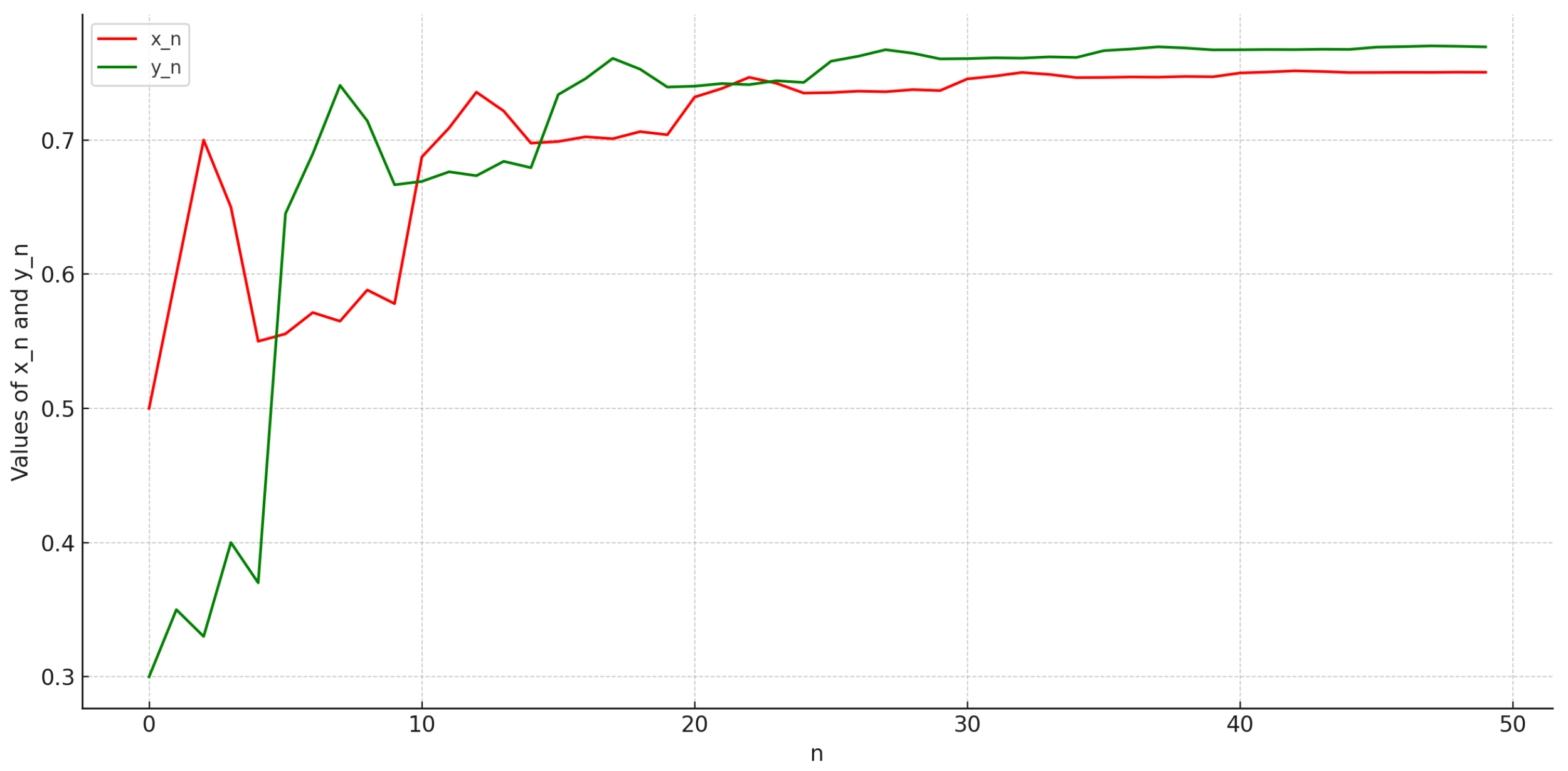
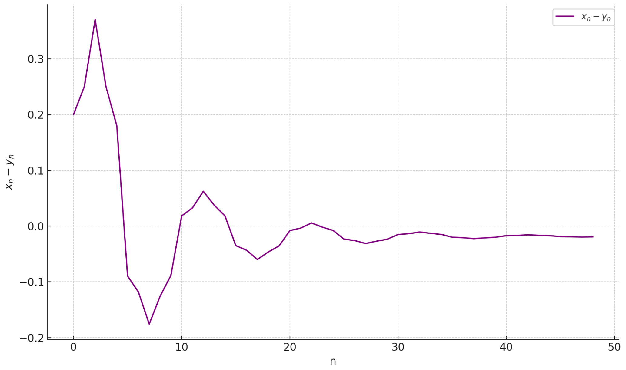
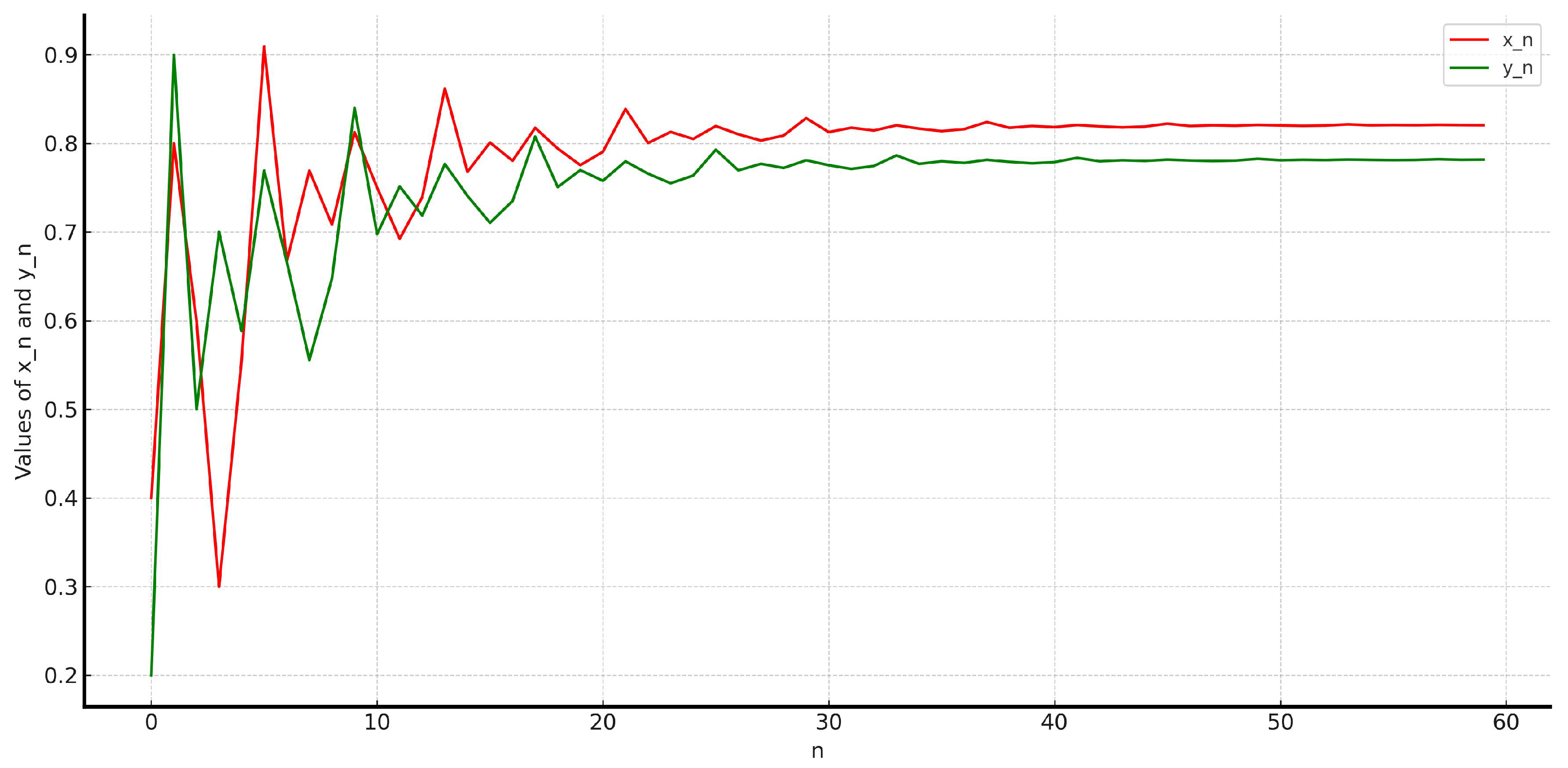
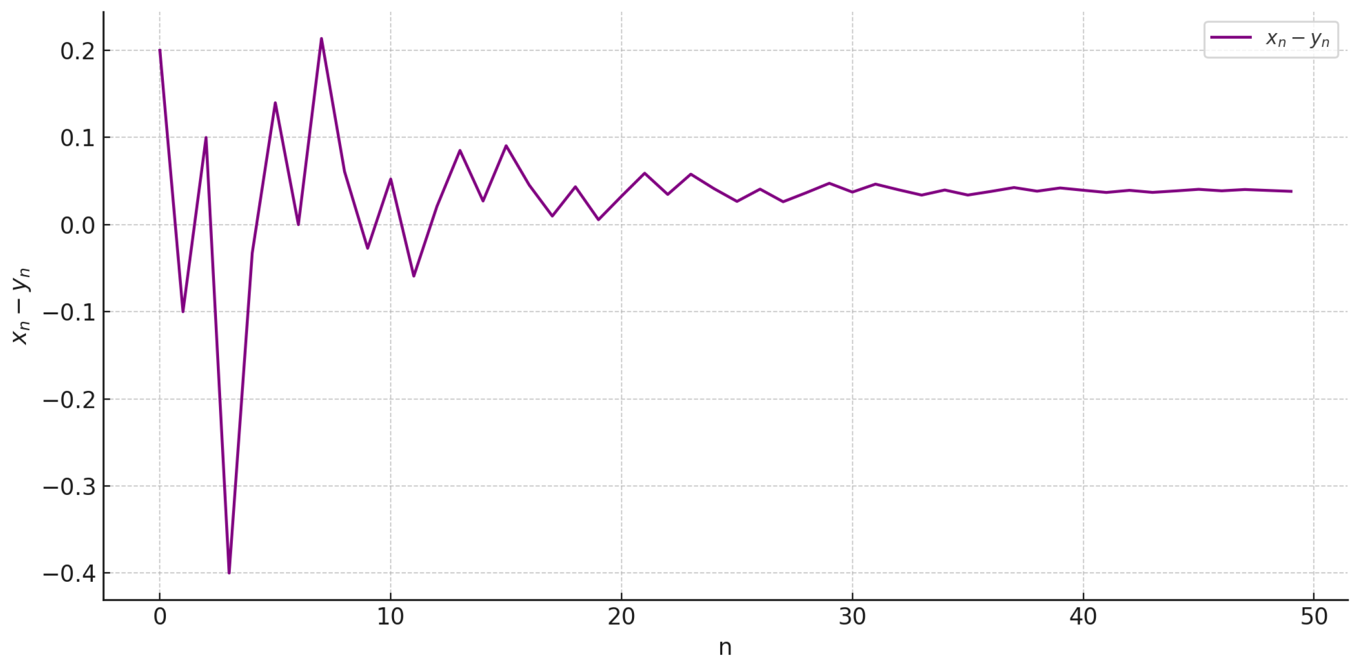
5. Numerical Examples

This section provides numerical simulations to illustrate the behavior of the nonlinear rational systems analyzed in the previous sections. By selecting specific values for the parameters and initial conditions, we demonstrate how the solutions evolve over time. The results confirm the theoretical findings, showing convergence to fixed points and highlighting the asymptotic stability of the system. Graphical representations are also included to provide a clearer view of the system’s dynamics.

Example 1. 

Let the following system of difference equations

$$x_{n+1}={\displaystyle \frac{1}{A-y_{n-k}}},y_{n+1}={\displaystyle \frac{1}{B-x_{n-k}}},n\ge 0,$$

(29)

where the parameters and initial conditions are chosen as follows:

• $A=2.1$, $B=2.05$, $k=5$, $x_0=0.5,x_1=0.6,x_2=0.7,x_3=0.65,x_4=0.55$, $y_0=0.3,y_1=0.35,y_2=0.33,y_3=0.4,y_4=0.37.$

The numerical results obtained for the variables $x_n$ and $y_n$ over the course of the first thirty iterations of the algorithm are comprehensively presented and summarized in Table 1. This table provides a clear overview of how the values of $x_n$ and $y_n$ evolve step by step during the early stages of the iterative process, offering valuable insights into the system’s dynamic behavior.

Table 1. Numerical values of $x_n$ and $y_n$ for the first 30 iterations of the System (29).

n	0	1	2	3	4	5	6	7
$x_n$	0.5000	0.6000	0.7000	0.6500	0.5500	0.5556	0.5714	0.5650
$y_n$	0.3000	0.3500	0.3300	0.4000	0.3700	0.6452	0.6897	0.7407
n	8	9	10	11	12	13	14	15
$x_n$	0.5882	0.5780	0.6874	0.7090	0.7357	0.7216	0.6977	0.6989
$y_n$	0.7143	0.6667	0.6691	0.6763	0.6734	0.6841	0.6794	0.7339
n	16	17	18	19	20	21	22	23
$x_n$	0.7024	0.7010	0.7063	0.7039	0.7320	0.7384	0.7467	0.7423
$y_n$	0.7457	0.7609	0.7528	0.7395	0.7401	0.7421	0.7413	0.7442
n	24	25	26	27	28	29	30	31
$x_n$	0.7350	0.7354	0.7364	0.7360	0.7376	0.7369	0.7456	0.7476
$y_n$	0.7429	0.7587	0.7624	0.7673	0.7647	0.7605	0.7607	0.7613

The following figures illustrate the numerical behavior of the nonlinear rational system (29). Figure 1 displays the time series plot of the variables $x_n$ and $y_n$, clearly demonstrating their convergence toward a stable equilibrium point. These visual representations provide concrete evidence of the system’s asymptotic behavior and support the theoretical results discussed earlier. Figure 2 shows the difference between the sequences $x_n$ and $y_n$ at each step n, illustrating how their values evolve and interact over time according to the given recursive system.

Figure 1. Plot of the numerical solution of the system (29).

Figure 2. Difference plot between $x_n$ and $y_n$ as solutions for the system (29).

Example 2. 

Let the following system of difference equations

$$x_{n+1}={\displaystyle \frac{1}{A-y_{n-k}}},y_{n+1}={\displaystyle \frac{1}{B-x_{n-k}}},n\ge 0,$$

(30)

where the parameters and initial conditions are chosen as follows:

• $A=2.0$, $B=2.1$, $k=4$, $x_0=0.4,x_1=0.8,x_2=0.6,x_3=0.3.$, $y_0=0.2,y_1=0.9,y_2=0.5,y_3=0.7.$

The numerical values of $x_n$ and $y_n$ for the first 23 iterations are summarized in Table 2.

Table 2. Numerical values of $x_n$ and $y_n$ for the first 23 iterations of the System (30).

n	0	1	2	3	4	5	6	7
$x_n$	0.4000	0.8000	0.6000	0.3000	0.5556	0.9091	0.6667	0.7692
$y_n$	0.2000	0.9000	0.5000	0.7000	0.5882	0.7692	0.6667	0.5556
n	8	9	10	11	12	13	14	15
$x_n$	0.7083	0.8125	0.7500	0.6923	0.7394	0.8618	0.7679	0.8009
$y_n$	0.6475	0.8397	0.6977	0.7514	0.7186	0.7767	0.7407	0.7104
n	16	17	18	19	20	21	22	23
$x_n$	0.7804	0.8175	0.7941	0.7754	0.7905	0.8387	0.8004	0.8129
$y_n$	0.7349	0.8077	0.7507	0.7698	0.7578	0.7797	0.7658	0.7550

The figures below depict the numerical dynamics of the nonlinear rational system (30). As shown in Figure 3, the time series plots of the variables $x_n$ and $y_n$ clearly indicate their convergence to a stable equilibrium point. These graphical representations offer tangible evidence of the system’s asymptotic behavior and reinforce the theoretical findings presented earlier. Meanwhile, Figure 4 shows the difference between the sequences $x_n$ and $y_n$ at each step n, illustrating how their values evolve and interact over time according to the given recursive system (30).

Figure 3. Plot of the numerical solution of the system (30).

Figure 4. Difference plot between $x_n$ and $y_n$ solution of the system (30).

6. Conclusions

In this paper, we investigated a class of nonlinear rational difference equations with delayed terms and analyzed their iterative behavior using an explicit analytical framework. The key contribution is the transformation of these nonlinear systems into second-order linear recurrence relations, enabling closed-form solutions. A generalized Balancing sequence was introduced to describe the system dynamics, extending classical sequences such as the standard Balancing numbers.

We proved the existence of two equilibrium points and established that one of them is globally asymptotically stable for all initial conditions. The analytical expression of the iterative solutions, in terms of generalized sequences, provides deep insights into the convergence and long-term behavior of the system. Numerical simulations supported the theoretical findings and demonstrated the stability and convergence toward the fixed point.

The analysis was conducted under the assumption of constant parameters and deterministic, autonomous dynamics. The current model does not account for the effects of external perturbations, randomness, or time-dependent coefficients, which may play a significant role in more general and realistic settings.

Future research may focus on extending this work in several directions. One promising avenue is to explore non-autonomous systems with time-varying parameters. Another is to incorporate stochastic elements into the model, addressing systems affected by noise or uncertainty. Finally, generalizing the approach to higher-order or multi-dimensional systems would broaden its applicability and practical relevance.

References

1. Kocic, V.L.; Ladas, G. Global Behavior of Nonlinear Difference Equations of Higher Order with Applications; Springer Science & Business Media: Dordrecht, The Netherlands, 1993; Volume 256. [Google Scholar]
2. Kulenovic, M.R.; Ladas, G. Dynamics of Second Order Rational Difference Equations: With Open Problems and Conjectures; Chapman and Hall/CRC: Boca Raton, FL, USA, 2001. [Google Scholar]
3. Amleh, A.M.; Camouzis, E.; Ladas, G. On the dynamics of a rational difference equation, part I. Int. J. Differ. Equ. 2008, 3, 1–35. [Google Scholar]
4. Elsayed, E.M. On a system of two nonlinear difference equations of order two. Proc. Jangjeon Math. Soc. 2015, 18, 353–368. [Google Scholar]
5. Elsayed, E.M. Solution for systems of difference equations of rational form of order two. Comput. Appl. Math. 2014, 33, 751–765. [Google Scholar] [CrossRef]
6. Elsayed, E.M. On the solutions and periodic nature of some systems of difference equations. Int. J. Biomath. 2014, 7, 1450067. [Google Scholar] [CrossRef]
7. Gümüş, M.; Soykan, Y. Global character of a six-dimensional nonlinear system of difference equations. Discret. Dyn. Nat. Soc. 2016, 55, 6842521. [Google Scholar] [CrossRef]
8. Gümüş, M. Analysis of periodicity for a new class of non-linear difference equations by using a new method. Electron. J. Math. Anal. Appl. 2020, 8, 109–116. [Google Scholar]
9. Gümüş, M. Global asymptotic behavior of a discrete system of difference equations with delays. Filomat 2023, 37, 251–264. [Google Scholar] [CrossRef]
10. Kara, M.; Yazlik, Y. Solvability of a system of nonlinear difference equations of higher order. Turk. J. Math. 2019, 43, 1533–1565. [Google Scholar] [CrossRef]
11. Kara, M.; Yazlik, Y.; Touafek, N.; Akrour, Y. On a three-dimensional system of difference equations with variable coefficients. J. Appl. Math. Inform. 2021, 39, 1533–1565. [Google Scholar]
12. Touafek, N. On a general system of difference equations defined by homogeneous functions. Math. Slovaca 2021, 71, 697–720. [Google Scholar] [CrossRef]
13. Yazlik, Y.; Tollu, D.T.; Taskara, N. Behaviour of solutions for a system of two higher-order difference equations. J. Sci. Arts 2018, 45, 813–826. [Google Scholar]
14. Yazlik, Y.; Kara, M. On a solvable system of difference equations of higher-order with period two coefficients. Commun. Fac. Sci. Univ. Ank. Ser. A1 Math. Stat. 2019, 68, 1675–1693. [Google Scholar] [CrossRef]
15. Wang, Z.; He, G.; Wang, Y.; Fan, J.; Zhang, Y.; Chai, Y.; Lu, S.J. Wave propagation in finite discrete chains unravelled by virtual measurement of dispersion properties. IET Sci. Meas. Technol. 2024, 18, 280–288. [Google Scholar] [CrossRef]
16. Guo, S.; Li, Y.; Wang, D. 2-Term Extended Rota–Baxter Pre-Lie -Algebra and Non-Abelian Extensions of Extended Rota–Baxter Pre-Lie Algebras. Result. Math. 2025, 80, 1–30. [Google Scholar] [CrossRef]
17. Yue, P. Uncertain Numbers. Mathematics 2025, 13, 496. [Google Scholar] [CrossRef]
18. Elsayed, E.M. Solutions of rational difference systems of order two. Math. Comput. Model. 2012, 55, 378–384. [Google Scholar] [CrossRef]
19. Li, W.; Sun, H. Dynamics of a rational difference equation. Appl. Math. Comput. 2005, 163, 577–591. [Google Scholar] [CrossRef]
20. Touafek, N. On a second order rational difference equation. Hacet. J. Math. Stat. 2012, 41, 867–874. [Google Scholar]
21. Halim, Y.; Bayram, M. On the solutions of a higher-order difference equation in terms of generalized Fibonacci sequences. Math. Methods Appl. Sci. 2016, 39, 2974–2982. [Google Scholar] [CrossRef]
22. Halim, Y. A system of difference equations with solutions associated to Fibonacci numbers. Int. J. Differ. Equ. 2016, 11, 65–77. [Google Scholar]
23. Hamioud, H.; Dekkar, I.; Touafek, N. Solvability of a third-order system of nonlinear difference equations via a generalized Fibonacci sequence. Miskolc Math. Notes 2024, 25, 271–285. [Google Scholar] [CrossRef]
24. Halim, Y.; Rabago, J.F.T. On the solutions of a second-order difference equations in terms of generalized Padovan sequences. Math. Slovaca 2018, 68, 625–638. [Google Scholar] [CrossRef]
25. Kara, M.; Yazlik, Y. On eight solvable systems of difference equations in terms of generalized Padovan sequences. Miskolc Math. Notes 2021, 22, 695–708. [Google Scholar] [CrossRef]
26. Kara, M.; Yazlik, Y. Representation of solutions of eight systems of difference equations via generalized Padovan sequences. Int. J. Nonlinear Anal. Appl. 2021, 12, 447–471. [Google Scholar]
27. Halim, Y.; Khelifa, A.; Berkal, M. Solutions of a system of two higher-order difference equations in terms of Lucas sequence. Univers. J. Math. Appl. 2019, 2, 202–211. [Google Scholar] [CrossRef]
28. Taşkara, N.; Büyük, H. On the solutions of three-dimensional difference equation systems via pell numbers. Avrupa Bilim Teknol. Derg. 2022, 34, 433–440. [Google Scholar] [CrossRef]
29. Kaouache, S.; Fečkan, M.; Halim, Y.; Khelifa, A. Theoretical analysis of higher-order system of difference equations with generalized balancing numbers. Math. Slovaca 2024, 74, 691–702. [Google Scholar] [CrossRef]
30. Arikoglu, A.; Ozkol, I. Solution of differential–difference equations by using differential transform method. Appl. Math. Comput. 2006, 181, 153–162. [Google Scholar] [CrossRef]
31. Bérczes, A.; Liptai, K.; Pink, I. On generalized balancing sequences. Fibonacci Q. 2010, 48, 121–128. [Google Scholar] [CrossRef]
Disclaimer/Publisher’s Note: The statements, opinions and data contained in all publications are solely those of the individual author(s) and contributor(s) and not of MDPI and/or the editor(s). MDPI and/or the editor(s) disclaim responsibility for any injury to people or property resulting from any ideas, methods, instructions or products referred to in the content.
Article Metrics
Citations
Article Access Statistics
Multiple requests from the same IP address are counted as one view.