On the Convergence Order of Jarratt-Type Methods for Nonlinear Equations

Abstract

The order of convergence for Jarratt-type methods in solving nonlinear equations is determined without relying on Taylor expansion. Unlike previous studies, we depend solely on assumptions about the derivatives of the involved operator up to the second order. The proof presented in this paper is independent of the Taylor series expansion, thereby reducing the need for assumptions about derivatives of higher order of the involved operator and enhancing the applicability of these methods. The method’s applicability is broadened by employing the concept of generalized conditions in local convergence analysis and majorizing sequences in semi-local analysis. This study includes numerical examples and basins of attraction for the methods.

1. Introduction

Several real-world problems can be mathematically modelled as an equation of the form

$$\mathcal{G}\left(v\right)=0,$$

(1)

where $\mathcal{G}:E\subseteq {\mathcal{B}}_1\to {\mathcal{B}}_2$ is a nonlinear operator mapping between the Banach spaces ${\mathcal{B}}_1$ and ${\mathcal{B}}_2$ and E is open convex set in ${\mathcal{B}}_1.$ One of the significant hurdles appearing in the real world is determining solutions $v^{\ast }$ of (1). Iterative methods are extensively used techniques for approximating solutions to equations that are nonlinear in nature, especially when exact solutions are not explicitly obtainable. Among the most widely used quadratically convergent iterative methods is Newton’s method (NM) as it converges rapidly from any sufficiently good initial guess. Even though this method provides a good convergence rate, the need to compute and invert the derivative of the given operator function in each of the iterative steps limits the applicability of this method. To overcome this, several Newton-like methods are available in the literature [1,2,3,4,5,6,7,8,9]. One such successful attempt was made by Ren et al. in [10], providing an iterative method of order six as in (2). Recall that a sequence $\left\{a_n\right\}$ in ${\mathcal{B}}_1$ with ${lim}_{n\to \infty }{a}_n=\alpha$ is known to be convergent of order $q>1$ if there exists a nonzero constant C such that

$$\begin{array}{c}\hfill \underset{n⟶\infty }{lim}{\displaystyle \frac{\parallel a_{n+1}-\alpha \parallel }{\parallel a_n{-\alpha \parallel }^q}}=C.\end{array}$$

Previous studies primarily used Taylor expansion to determine the order of convergence, which necessitates the existence of derivatives, mostly of higher order. An alternative method involves employing the computational order of convergence (COC) [11], defined as follows:

$$\overline{\rho }={\displaystyle \frac{ln\left(∥{\displaystyle \frac{a_{n+1}-\alpha }{a_n-\alpha }}∥\right)}{ln\left(∥{\displaystyle \frac{a_n-\alpha }{a_{n-1}-\alpha }}∥\right)}},$$

where $a_{n-1},a_n,$ and $a_{n+1}$ are three consecutive iterates near root $\alpha$ or the approximate computational order of convergence (ACOC) defined as

$$\overline{\rho }={\displaystyle \frac{ln\left(∥{\displaystyle \frac{a_{n+1}-a_n}{a_n-a_{n-1}}}∥\right)}{ln\left(∥{\displaystyle \frac{a_n-a_{n-1}}{a_{n-1}-a_{n-2}}}∥\right)}},$$

where $a_{n-2}, a_{n-1}, a_n,$ and $a_{n+1}$ are four consecutive iterates near root $\alpha$, used to obtain the order of convergence.

The limitation of COC and ACOC for iterative methods lies in their susceptibility to the oscillating behavior of approximations and slow convergence during early iterations [12]. As a result, in general, COC and ACOC precisely do not accurately reflect the actual convergence order.

In [10], Ren et al., considered the following iterative scheme:

$$\begin{array}{ccc}{w}_n\hfill & =\hfill & v_n-{\displaystyle \frac{2}{3}}{\mathcal{A}}^{\prime }{\left(v_n\right)}^{-1}\mathcal{A}\left(v_n\right),\hfill \\ z_n\hfill & =\hfill & v_n-{\displaystyle \frac{1}{2}}{[3{\mathcal{A}}^{\prime }\left(w_n\right)-{\mathcal{A}}^{\prime }\left(v_n\right)]}^{-1}[3{\mathcal{A}}^{\prime }\left(w_n\right)+{\mathcal{A}}^{\prime }\left(v_n\right)]{\mathcal{A}}^{\prime }{\left(v_n\right)}^{-1}\mathcal{A}\left(v_n\right),\hfill \\ v_{n+1}\hfill & =\hfill & z_n-{\mathcal{A}}^{\prime }{\left(z_n\right)}^{-1}\mathcal{A}\left(z_n\right),\forall n=0,1,2,3...\hfill \end{array}$$

(2)

for solving (1), when ${\mathcal{B}}_1={\mathcal{B}}_2={\mathbb{R}}^k.$

In [10], Taylor’s expansion is used to achieve a sixth-order convergence, but the analysis requires conditions on the derivatives of $\mathcal{A}$ up to the seventh order. These assumptions restrict the applicability of the method given in (2) to problems involving operators that are differentiable at least seven times.

In this work, we initially determine the order of convergence of the scheme (refer to [8,13]) described for all $n=0,1,2,\dots$ as follows:

$$\begin{array}{ccc}{w}_n\hfill & =\hfill & v_n-{\displaystyle \frac{2}{3}}{\mathcal{A}}^{\prime }{\left(v_n\right)}^{-1}\mathcal{A}\left(v_n\right),\hfill \\ v_{n+1}\hfill & =\hfill & v_n-{\displaystyle \frac{1}{2}}{[3{\mathcal{A}}^{\prime }\left(w_n\right)-{\mathcal{A}}^{\prime }\left(v_n\right)]}^{-1}[3{\mathcal{A}}^{\prime }\left(w_n\right)+{\mathcal{A}}^{\prime }\left(v_n\right)]{\mathcal{A}}^{\prime }{\left(v_n\right)}^{-1}\mathcal{A}\left(v_n\right),\hfill \end{array}$$

(3)

where ${\mathcal{B}}_1$ and ${\mathcal{B}}_2$ are Banach spaces.

Additionally, we enhance the method to a fifth-order approach, given as

$$\begin{array}{ccc}{w}_n\hfill & =\hfill & v_n-{\displaystyle \frac{2}{3}}{\mathcal{A}}^{\prime }{\left(v_n\right)}^{-1}\mathcal{A}\left(v_n\right),\hfill \\ z_n\hfill & =\hfill & v_n-{\displaystyle \frac{1}{2}}{[3{\mathcal{A}}^{\prime }\left(w_n\right)-{\mathcal{A}}^{\prime }\left(v_n\right)]}^{-1}[3{\mathcal{A}}^{\prime }\left(w_n\right)+{\mathcal{A}}^{\prime }\left(v_n\right)]{\mathcal{A}}^{\prime }{\left(v_n\right)}^{-1}\mathcal{A}\left(v_n\right),\hfill \\ v_{n+1}\hfill & =\hfill & z_n-{\mathcal{A}}^{\prime }{\left({\displaystyle \frac{3w_n-v_n}{2}}\right)}^{-1}\mathcal{A}\left(z_n\right),n=0,1,2,3...,\hfill \end{array}$$

(4)

in Section 4.

In Section 2, we establish a third-order convergence for Method (3), and in Section 3, we demonstrate a sixth-order convergence for (2), relying on assumptions about the derivatives of $\mathcal{A}$ up to the second order. Consequently, our analysis broadens the applicability of methods (3), (2), and (4) to problems that could not be addressed using the approaches in [10,14,15,16,17].

In Section 5, we examine the constraints of our approach and propose novel strategies to overcome these limitations for both local and semi-local convergence scenarios. The convergence conditions are solely tied to the operators involved in the method for both the semi-local and local cases.

The remaining part of the paper includes the efficiency index in Section 6, a numerical demonstration in Section 7, and basins of attraction in Section 8, concluding with a summary in Section 9.

2. Convergence Order of Iterative Scheme (3)

The analysis of local convergence relies on the following assumptions:

(A1)

${\mathcal{A}}^{\prime }{\left(v^{\ast }\right)}^{-1}$ exists and ∃$L_0>0$ such that $\forall v,w\in E,$

$$\parallel {\mathcal{A}}^{\prime }{\left(v^{\ast }\right)}^{-1}({\mathcal{A}}^{\prime }\left(v\right)-{\mathcal{A}}^{\prime }\left(w\right))\parallel \le L_0\parallel v-w\parallel .$$

(A2)

∃$L_1>0$ such that $\forall v,w\in E,$

$$\parallel {\mathcal{A}}^{\prime }{\left(v^{\ast }\right)}^{-1}({\mathcal{A}}^{″}\left(v\right)-{\mathcal{A}}^{″}\left(w\right))\parallel \le L_1\parallel v-w\parallel .$$

(A3)

∃$L_2>0$ such that

$$\parallel {\mathcal{A}}^{\prime }{\left(v^{\ast }\right)}^{-1}{\mathcal{A}}^{″}\left(v\right)\parallel \le L_2,\forall v\in E.$$

and

(A4)

∃$L_3>0$ such that

$$\parallel {\mathcal{A}}^{\prime }{\left(v^{\ast }\right)}^{-1}{\mathcal{A}}^{\prime }\left(v\right)\parallel \le L_3,\forall v\in E.$$

Using the constants $L_0,L_1,L_2$, and $L_3$, we define continuous nondecreasing functions (CNF)${\mathsf{\Theta }}_1,H_1:[0,{\displaystyle \frac{1}{L_0}})⟶\mathbb{R}$ as follows:

$$\begin{array}{ccc}\hfill {\mathsf{\Theta }}_1\left(t\right)& =& {\displaystyle \frac{L_0}{2}}(3(1+{\displaystyle \frac{2L_3}{3(1-L_{0}t)}})+1)t\hfill \end{array}$$

and

$$H_1\left(t\right)={\mathsf{\Theta }}_1\left(t\right)-1.$$

Note that $H_1\left(0\right)=-1$ and if $H_1\left(t\right)$ approaches ∞ as t tends to ${{\displaystyle \frac{1}{L_0}}}^{-}$, then $H_1\left(t\right)=0$ possesses a smallest positive root in $[0,{\displaystyle \frac{1}{L_0}})$, which is denoted by $\lambda$. Define CNF $g_1,h_1:[0,\lambda )⟶\mathbb{R}$ by

$$\begin{array}{ccc}\hfill g_1\left(t\right)& =& {\displaystyle \frac{1}{48(1-{\mathsf{\Theta }}_1\left(t\right)){(1-L_{0}t)}^2}}\hfill \\ & & \times [(93(L_1-L_{0}t)+32L_1{L}_3+36L_0{L}_2)(1-L_{0}t)+12L_0{L}_2{L}_3]\hfill \end{array}$$

and

$$h_1\left(t\right)=g_1\left(t\right)t^2-1.$$

As $h_1\left(0\right)=-1$ and $h_1\left(t\right)$ approaches ∞ as $t\to {\lambda }^{-}$, there exists a smallest root of $h_1\left(t\right)=0$ in $[0,\lambda )$, which we call ${\lambda }_1$.

So

$$r=min\{{\lambda }_1,{\displaystyle \frac{1}{2L_0}},1\}.$$

(5)

Then, we have

$$0\le g_1\left(t\right)t^2<1,\forall t\in [0,r).$$

(6)

Throughout the paper, we consider $B(v_0,\rho )$ and $B[v_0,\rho ]$ as open and closed balls, respectively, centered at $v_0\in X$ with radius $\rho >0.$

Theorem 1. 

Assuming (A1)–(A4) are true, the sequence $\left\{v_n\right\}$ given by (3) with initial value $v_0\in B(v^{\ast },r)$ converges to $v^{\ast }$, and the following estimate is valid:

$$\parallel v_{n+1}-v^{\ast }\parallel \le g_1\left(r\right){\parallel v_n-v^{\ast }\parallel }^3.$$

(7)

Proof. 

An inductive argument will be employed for the proof. As a first step, we will demonstrate that the operator $3{\mathcal{A}}^{\prime }\left(w\right)-{\mathcal{A}}^{\prime }\left(v\right)$ is invertible for all v and w belonging to the open ball $B(v^{\ast },r).$ Note that, by (A1), we have

$$\begin{array}{ccc}\parallel {\left(2{\mathcal{A}}^{\prime }\left(v^{\ast }\right)\right)}^{-1}(3{\mathcal{A}}^{\prime }\left(w\right)-{\mathcal{A}}^{\prime }\left(v\right)-2{\mathcal{A}}^{\prime }\left(v^{\ast }\right))\parallel \hfill & \le \hfill & {\displaystyle \frac{3}{2}}\parallel {\mathcal{A}}^{\prime }{\left(v^{\ast }\right)}^{-1}({\mathcal{A}}^{\prime }\left(w\right)-{\mathcal{A}}^{\prime }\left(v^{\ast }\right))\parallel \hfill \\ \hfill & \hfill & +{\displaystyle \frac{1}{2}}\parallel {\mathcal{A}}^{\prime }{\left(v^{\ast }\right)}^{-1}({\mathcal{A}}^{\prime }\left(v\right)-{\mathcal{A}}^{\prime }\left(v^{\ast }\right))\parallel \hfill \\ \hfill & \le \hfill & {\displaystyle \frac{L_0}{2}}(3\parallel w-v^{\ast }\parallel +\parallel v-v^{\ast }\parallel )\hfill \\ \hfill & \le \hfill & {\displaystyle \frac{3}{2}}{L}_{0}r+{\displaystyle \frac{1}{2}}{L}_{0}r=2L_{0}r<1.\hfill \end{array}$$

(8)

Therefore, by applying Banach’s Lemma (BL) on the invertibility of operators, $3{\mathcal{A}}^{\prime }\left(w\right)-{\mathcal{A}}^{\prime }\left(v\right)$ is invertible and by (8), we have

$$\parallel {(3{\mathcal{A}}^{\prime }\left(w\right)-{\mathcal{A}}^{\prime }\left(v\right))}^{-1}{\mathcal{A}}^{\prime }\left(v^{\ast }\right)\parallel \le {\displaystyle \frac{1}{2(1-\frac{L_0}{2}(3\parallel w-v^{\ast }\parallel +\parallel v-v^{\ast }\parallel \left)\right)}}.$$

(9)

Similarly, one can prove that

$$\parallel {\mathcal{A}}^{\prime }{\left(v\right)}^{-1}{\mathcal{A}}^{\prime }\left(v^{\ast }\right)\parallel \le {\displaystyle \frac{1}{1-L_0\parallel v-v^{\ast }\parallel }}.$$

(10)

Next, by Method (3), we have

$$\begin{array}{ccc}{v}_1-v^{\ast }\hfill & =\hfill & v_0-v^{\ast }-{\displaystyle \frac{1}{2}}{(3{\mathcal{A}}^{\prime }\left(w_0\right)-{\mathcal{A}}^{\prime }\left(v_0\right))}^{-1}(3{\mathcal{A}}^{\prime }\left(w_0\right)+{\mathcal{A}}^{\prime }\left(v_0\right)){\mathcal{A}}^{\prime }{\left(v_0\right)}^{-1}\mathcal{A}\left(v_0\right)\hfill \\ \hfill & =\hfill & {(3{\mathcal{A}}^{\prime }\left(w_0\right)-{\mathcal{A}}^{\prime }\left(v_0\right))}^{-1}[(3{\mathcal{A}}^{\prime }\left(w_0\right)-{\mathcal{A}}^{\prime }\left(v_0\right))(v_0-v^{\ast })\hfill \\ \hfill & \hfill & -{\displaystyle \frac{1}{2}}(3{\mathcal{A}}^{\prime }\left(w_0\right)+{\mathcal{A}}^{\prime }\left(v_0\right)){\mathcal{A}}^{\prime }{\left(v_0\right)}^{-1}\mathcal{A}\left(v_0\right)].\hfill \end{array}$$

(11)

For convenience, let $P={(3{\mathcal{A}}^{\prime }\left(w_0\right)-{\mathcal{A}}^{\prime }\left(v_0\right))}^{-1}.$ In order to prove (7), we rearrange the Equation (11) as follows:

$$\begin{array}{ccc}{v}_1-v^{\ast }\hfill & =\hfill & P\left\{[(3{\mathcal{A}}^{\prime }\left(w_0\right)-{\mathcal{A}}^{\prime }\left(v_0\right))-2\mathcal{A}\left(v_0\right)\right.\hfill \\ \hfill & \hfill & +\left.(2I-{\displaystyle \frac{1}{2}}(3{\mathcal{A}}^{\prime }\left(w_0\right)+{\mathcal{A}}^{\prime }\left(v_0\right)){\mathcal{A}}^{\prime }{\left(v_0\right)}^{-1})\mathcal{A}\left(v_0\right)\right\}\hfill \\ \hfill & =\hfill & P\left\{3{\int }_0^1{\int }_0^1{\mathcal{A}}^{″}(v^{\ast }+t(v_0-v^{\ast })+\theta (w_0-v^{\ast }-t(v_0-v^{\ast })))d\theta \right.\hfill \\ \hfill & \hfill & \times (w_0-v^{\ast }-t(v_0-v^{\ast }))dt(v_0-v^{\ast })\hfill \\ \hfill & \hfill & -{\int }_0^1{\int }_0^1{\mathcal{A}}^{″}(v^{\ast }+t(v_0-v^{\ast })+\theta (1-t)(v_0-v^{\ast }))dt(1-t){(v_0-v^{\ast })}^2\hfill \\ \hfill & \hfill & +\left.{\displaystyle \frac{3}{2}}{\int }_0^1{\mathcal{A}}^{″}(w_0+\theta (v_0-w_0))d\theta (v_0-w_0){\mathcal{A}}^{\prime }{\left(v_0\right)}^{-1}\mathcal{A}\left(v_0\right)\right\}\hfill \\ \hfill & =\hfill & P\left\{3{\int }_0^1{\int }_0^1{\mathcal{A}}^{″}(v^{\ast }+t(v_0-v^{\ast })+\theta (w_0-v^{\ast }-t(v_0-v^{\ast })))d\theta \right.\hfill \\ \hfill & \hfill & \times \left(({\displaystyle \frac{1}{3}}-t){(v_0-v^{\ast })}^2\right)dt\hfill \\ \hfill & \hfill & +3{\int }_0^1{\int }_0^1{\mathcal{A}}^{″}(v^{\ast }+t(v_0-v^{\ast })+\theta (w_0-v^{\ast }-t(v_0-v^{\ast })))d\theta \hfill \\ \hfill & \hfill & \times {\displaystyle \frac{2}{3}}(v_0-v^{\ast }-{\mathcal{A}}^{\prime }{\left(v_0\right)}^{-1}\mathcal{A}\left(v_0\right))dt(v_0-v^{\ast })\hfill \\ \hfill & \hfill & (\mathrm{because}{w}_0-v^{\ast }={\displaystyle \frac{1}{3}}(v_0-v^{\ast })+{\displaystyle \frac{2}{3}}(v_0-v^{\ast }-{\mathcal{A}}^{\prime }{\left(v_0\right)}^{-1}\mathcal{A}\left(v_0\right)))\hfill \\ \hfill & \hfill & -{\int }_0^1{\int }_0^1{\mathcal{A}}^{″}(v^{\ast }+t(v_0-v^{\ast })+\theta (1-t)(v_0-v^{\ast }))dt(1-t){(v_0-v^{\ast })}^2\hfill \\ \hfill & \hfill & +\left.{\int }_0^1{\mathcal{A}}^{″}(w_0+\theta (v_0-w_0))d\theta {\left({\mathcal{A}}^{\prime }{\left(v_0\right)}^{-1}\mathcal{A}\left(v_0\right)\right)}^2\right\}.\hfill \end{array}$$

(12)

Let $S_1(\theta ,t)={\mathcal{A}}^{″}(v^{\ast }+t(v_0-v^{\ast })+\theta (w_0-v^{\ast }-t(v_0-v^{\ast }))),$$S_2(\theta ,t)={\mathcal{A}}^{″}(v^{\ast }+t(v_0-v^{\ast })+\theta (1-t)(v_0-v^{\ast }))$, and $S_3\left(\theta \right)={\mathcal{A}}^{″}(w_0+\theta (v_0-w_0)).$ Then, by (12), we have

$$\begin{array}{ccc}{v}_1-v^{\ast }\hfill & =\hfill & P\left\{{\int }_0^1{\int }_0^1{S}_1(\theta ,t)d\theta \left((1-2t){(v_0-v^{\ast })}^2\right)dt\right.\hfill \\ \hfill & \hfill & +2{\int }_0^1{\int }_0^1{S}_1(\theta ,t)d\theta dt\hfill \\ \hfill & \hfill & \times {\mathcal{A}}^{\prime }{\left(v_0\right)}^{-1}({\mathcal{A}}^{\prime }\left(v_0\right)-{\int }_0^1{\mathcal{A}}^{\prime }(v^{\ast }+\tau (v_0-v^{\ast }))d\tau ){(v_0-v^{\ast })}^2\hfill \\ \hfill & \hfill & -{\int }_0^1{\int }_0^1{S}_2(\theta ,t)d\theta dt{(v_0-v^{\ast })}^2\hfill \\ \hfill & \hfill & +{\int }_0^1{\int }_0^1(S_2(\theta ,t)-S_1(\theta ,t))tdt{(v_0-v^{\ast })}^{2}d\theta \hfill \\ \hfill & \hfill & +\left.{\int }_0^1{S}_3\left(\theta \right)d\theta {\left({\mathcal{A}}^{\prime }{\left(v_0\right)}^{-1}\mathcal{A}\left(v_0\right)\right)}^2\right\}\hfill \\ \hfill & =:\hfill & I_1+I_2+I_3+I_4+I_5,\hfill \end{array}$$

(13)

where

$$\begin{array}{ccc}\hfill I_1& =& P{\int }_0^1{\int }_0^1{S}_1(\theta ,t)d\theta \left((1-2t){(v_0-v^{\ast })}^2\right)dt,\hfill \\ \hfill I_2& =& 2P{\int }_0^1{\int }_0^1{S}_1(\theta ,t)d\theta dt{\mathcal{A}}^{\prime }{\left(v_0\right)}^{-1}({\mathcal{A}}^{\prime }\left(v_0\right)-{\int }_0^1{\mathcal{A}}^{\prime }(v^{\ast }+\tau (v_0-v^{\ast }))d\tau ){(v_0-v^{\ast })}^2,\hfill \\ \hfill I_3& =& P{\int }_0^1{\int }_0^1(S_2(\theta ,t)-S_1(\theta ,t))tdt{(v_0-v^{\ast })}^{2}d\theta ,\hfill \\ \hfill I_4& =& P{\int }_0^1{\int }_0^1(S_3\left(\theta \right)-S_2(\theta ,t))d\theta dt{(v_0-v^{\ast })}^2\hfill \end{array}$$

and

$$I_5=P{\int }_0^1{S}_3\left(\theta \right)d\theta [{\left({\mathcal{A}}^{\prime }{\left(v_0\right)}^{-1}{\int }_0^1{\mathcal{A}}^{\prime }(v^{\ast }+\tau (v_0-v^{\ast }))\right)}^2-I]{(v_0-v^{\ast })}^2.$$

Next, we estimate the norms of $I_1,I_2,I_3,I_4$, and $I_5.$ Note that

$$\begin{array}{ccc}\parallel I_1\parallel \hfill & =\hfill & ∥P{\int }_0^1{\int }_0^1{S}_1(\theta ,t)d\theta (1-2t){(v_0-v^{\ast })}^{2}dt∥\hfill \\ \hfill & \le \hfill & \parallel P{\mathcal{A}}^{\prime }\left(v^{\ast }\right)\parallel {\int }_0^1{\int }_0^1\parallel {\mathcal{A}}^{\prime }{\left(v^{\ast }\right)}^{-1}[{\mathcal{A}}^{″}(v^{\ast }+t(v_0-v^{\ast })+\theta (w_0-v^{\ast }-t(v_0-v^{\ast })))\hfill \\ \hfill & \hfill & -{\mathcal{A}}^{″}\left(v^{\ast }\right)]\parallel d\theta |1-2t|{\parallel v_0-v^{\ast }\parallel }^{2}dt\hfill \\ \hfill & \hfill & +\parallel {(3{\mathcal{A}}^{\prime }\left(w_0\right)-{\mathcal{A}}^{\prime }\left(v_0\right))}^{-1}{\mathcal{A}}^{″}\left(v^{\ast }\right){\int }_0^1(1-2t){(v_0-v^{\ast })}^{2}dt\parallel \hfill \\ \hfill & \le \hfill & L_1\parallel P{\mathcal{A}}^{\prime }\left(v^{\ast }\right)\parallel {\int }_0^1{\int }_0^1\parallel t(v_0-v^{\ast })+\theta (w_0-v^{\ast }-t(v_0-v^{\ast }))\parallel \hfill \\ \hfill & \hfill & \times |1-2t|{\parallel v_0-v^{\ast }\parallel }^{2}d\theta dt\hfill \\ \hfill & \le \hfill & L_1\parallel P{\mathcal{A}}^{\prime }\left(v^{\ast }\right)\parallel \left[{\int }_0^1{\displaystyle \frac{3\left|t\right||1-2t|}{2}}\parallel v_0-v^{\ast }\parallel +{\displaystyle \frac{|1-2t|}{2}}\parallel w_0-v^{\ast }\parallel \right]{\parallel v_0-v^{\ast }\parallel }^{2}d\theta dt\hfill \\ \hfill & \le \hfill & L_1\parallel P{\mathcal{A}}^{\prime }\left(v^{\ast }\right)\parallel \left[{\displaystyle \frac{3}{8}}{\parallel v_0-v^{\ast }\parallel }^3+{\displaystyle \frac{1}{4}}\parallel w_0-v^{\ast }\parallel {\parallel v_0-v^{\ast }\parallel }^2\right],\hfill \end{array}$$

(14)

which is obtained using (A2) and (10) (with $v=v_0$). Note that $\parallel w_0-v^{\ast }\parallel \le \parallel w_0-v_0\parallel + \parallel v_0-v^{\ast }\parallel$, and using (10), we have

$$\begin{array}{ccc}\parallel w_0-v_0\parallel \hfill & =\hfill & \parallel {\displaystyle \frac{2}{3}}{\mathcal{A}}^{\prime }{\left(v_0\right)}^{-1}\mathcal{A}\left(v_0\right)\parallel \hfill \\ \hfill & \le \hfill & {\displaystyle \frac{2}{3}}\parallel {\mathcal{A}}^{\prime }{\left(v_0\right)}^{-1}{\mathcal{A}}^{\prime }\left(v^{\ast }\right)\parallel \parallel {\int }_0^1{\mathcal{A}}^{\prime }{\left(v^{\ast }\right)}^{-1}{\mathcal{A}}^{\prime }(v^{\ast }+t(v_0-v^{\ast }))dt(v_0-v^{\ast })\parallel \hfill \\ \hfill & \le \hfill & {\displaystyle \frac{2L_3}{3(1-L_0\parallel v_0-v^{\ast }\parallel )}}\parallel v_0-v^{\ast }\parallel .\hfill \end{array}$$

(15)

Therefore,

$$\parallel w_0-v^{\ast }\parallel \le \left(1+{\displaystyle \frac{2L_3}{3(1-L_0\parallel v_0-v^{\ast }\parallel )}}\right)\parallel v_0-v^{\ast }\parallel$$

(16)

and hence by (9) (with $w=w_0$ and $v=v_0$), we have

$$\parallel P{\mathcal{A}}^{\prime }\left(v^{\ast }\right)\parallel \le {\displaystyle \frac{1}{2(1-\frac{L_0}{2}(3(1+\frac{2L_3}{3(1-L_0\parallel v_0-v^{\ast }\parallel )})+1)\parallel v-v^{\ast }\parallel )}}.$$

(17)

Therefore, using (16) in (14), we obtain

$$\begin{array}{ccc}\parallel I_1\parallel \hfill & \le \hfill & {\displaystyle \frac{L_1(3+2(1+\frac{2L_3}{3(1-L_0\parallel v_0-v^{\ast }\parallel )}))}{16(1-\frac{L_0}{2}(3(1+\frac{2L_3}{3(1-L_0\parallel v_0-v^{\ast }\parallel )})+1)\parallel v_0-v^{\ast }\parallel )}}{\parallel v_0-v^{\ast }\parallel }^3.\hfill \\ \hfill \end{array}$$

(18)

Next,

$$\begin{array}{ccc}\parallel I_2\parallel \hfill & =\hfill & \parallel 2P{\mathcal{A}}^{\prime }\left(v^{\ast }\right)\parallel ∥{\int }_0^1{\int }_0^1{\mathcal{A}}^{\prime }{\left(v^{\ast }\right)}^{-1}{S}_1(\theta ,t)d\theta dt{\mathcal{A}}^{\prime }{\left(v_0\right)}^{-1}{\mathcal{A}}^{\prime }\left(v^{\ast }\right)\hfill \\ \hfill & \hfill & \times {\int }_0^1{\mathcal{A}}^{\prime }{\left(v^{\ast }\right)}^{-1}({\mathcal{A}}^{\prime }\left(v_0\right)-{\mathcal{A}}^{\prime }(v^{\ast }+\tau (v_0-v^{\ast })))d\tau {(v_0-v^{\ast })}^2∥\hfill \end{array}$$

and by (9), (10), (A1), and (A3), we have

$$\parallel I_2\parallel \le {\displaystyle \frac{L_0{L}_2}{2(1-\frac{L_0}{2}(3(1+\frac{2L_3}{3(1-L_0\parallel v_0-v^{\ast }\parallel )})+1)\parallel v_0-v^{\ast }\parallel \left)\right(1-L_0\parallel v_0-v^{\ast }\parallel )}}{\parallel v_0-v^{\ast }\parallel }^3.$$

(19)

By using (9) and (A2), we have

$$\begin{array}{ccc}\parallel I_3\parallel \hfill & \le \hfill & {\displaystyle \frac{L_1}{8(1-\frac{L_0}{2}(3(1+\frac{2L_3}{3(1-L_0\parallel v_0-v^{\ast }\parallel )})+1)\parallel v_0-v^{\ast }\parallel )}}\hfill \\ \hfill & \hfill & \times (\parallel v_0-v^{\ast }\parallel +\parallel w_0-v^{\ast }\parallel )\parallel v_0-v^{\ast }{\parallel }^2.\hfill \end{array}$$

(20)

Thus, by (15) and (16), we have

$$\begin{array}{ccc}\parallel I_3\parallel \hfill & \le \hfill & {\displaystyle \frac{L_1}{8(1-\frac{L_0}{2}(3(1+\frac{2L_3}{3(1-L_0\parallel v_0-v^{\ast }\parallel )})+1)\parallel v_0-v^{\ast }\parallel )}}\hfill \\ \hfill & \hfill & \times \left(2+{\displaystyle \frac{2L_3}{3(1-L_0\parallel v_0-v^{\ast }\parallel )}}\right){\parallel v_0-v^{\ast }\parallel }^3\hfill \\ \hfill & \le \hfill & {\displaystyle \frac{L_1\left(3\right(1-L_0\parallel v_0-v^{\ast }\parallel )+L_3)}{12(1-\frac{L_0}{2}(3(1+\frac{2L_3}{3(1-L_0\parallel v_0-v^{\ast }\parallel )})+1)\parallel v_0-v^{\ast }\parallel \left)\right(1-L_0\parallel v_0-v^{\ast }\parallel )}}{\parallel v_0-v^{\ast }\parallel }^3.\hfill \end{array}$$

(21)

Similarly, we have

$$\begin{array}{ccc}\hfill \parallel I_4\parallel & =& \parallel P{\mathcal{A}}^{\prime }\left(v^{\ast }\right){\int }_0^1{\int }_0^1{\mathcal{A}}^{\prime }{\left(v^{\ast }\right)}^{-1}(S_3\left(\theta \right)-S_2(\theta ,t))d\theta dt{(v_0-v^{\ast })}^2\parallel \hfill \\ & \le & {\displaystyle \frac{L_1}{2(1-\frac{L_0}{2}(3(1+\frac{2L_3}{3(1-L_0\parallel v_0-v^{\ast }\parallel )})+1)\parallel v_0-v^{\ast }\parallel )}}\hfill \\ & & \times ({\displaystyle \frac{3}{4}}\parallel v_0-v^{\ast }\parallel +\parallel w_0-v^{\ast }\parallel +{\displaystyle \frac{1}{2}}\parallel v_0-w_0\parallel )\parallel v_0-v^{\ast }{\parallel }^2.\hfill \end{array}$$

So, by using (15) and (16), we have

$$\begin{array}{ccc}\parallel I_4\parallel \hfill & \le \hfill & {\displaystyle \frac{L_1}{2(1-\frac{L_0}{2}(3(1+\frac{2L_3}{3(1-L_0\parallel v_0-v^{\ast }\parallel )})+1)\parallel v_0-v^{\ast }\parallel )}}\hfill \\ \hfill & \hfill & \times \left({\displaystyle \frac{5}{4}}+{\displaystyle \frac{3}{2}}(1+{\displaystyle \frac{2L_3}{3(1-L_0\parallel v_0-v^{\ast }\parallel )}})\right){\parallel v_0-v^{\ast }\parallel }^3\hfill \\ \hfill & =\hfill & {\displaystyle \frac{L_1(11-11L_0\parallel v_0-v^{\ast }\parallel +4L_3)}{8(1-\frac{L_0}{2}(3(1+\frac{2L_3}{3(1-L_0\parallel v_0-v^{\ast }\parallel )})+1)\parallel v_0-v^{\ast }\parallel \left)\right(1-L_0\parallel v_0-v^{\ast }\parallel )}}{\parallel v_0-v^{\ast }\parallel }^3.\hfill \end{array}$$

(22)

Next, we shall obtain an estimate for $\parallel I_5\parallel .$ Observe that

$$\begin{array}{ccc}\hfill \parallel I_5\parallel & =& \parallel P{\mathcal{A}}^{\prime }\left(v^{\ast }\right){\int }_0^1{\mathcal{A}}^{\prime }{\left(v^{\ast }\right)}^{-1}{S}_3\left(\theta \right)d\theta \hfill \\ & & \times \left[{\left({\mathcal{A}}^{\prime }{\left(v_0\right)}^{-1}{\int }_0^1{\mathcal{A}}^{\prime }(v^{\ast }+\tau (v_0-v^{\ast }))d\tau \right)}^2-I\right]{(v_0-v^{\ast })}^2\parallel \hfill \\ & \le & \parallel P{\mathcal{A}}^{\prime }\left(v^{\ast }\right)\parallel \parallel {\mathcal{A}}^{\prime }{\left(v^{\ast }\right)}^{-1}{S}_3\left(\theta \right)\parallel \parallel {\mathcal{A}}^{\prime }{\left(v_0\right)}^{-1}{\mathcal{A}}^{\prime }\left(v^{\ast }\right)\parallel \hfill \\ & & \times \left[{\int }_0^1\parallel {\mathcal{A}}^{\prime }{\left(v^{\ast }\right)}^{-1}({\mathcal{A}}^{\prime }(v^{\ast }+\tau (v_0-v^{\ast }))-{\mathcal{A}}^{\prime }\left(v_0\right))\parallel d\tau \right.\hfill \\ & & +{\int }_0^1\parallel {\mathcal{A}}^{\prime }{\left(v^{\ast }\right)}^{-1}{\mathcal{A}}^{\prime }(v^{\ast }+\tau (v_0-v^{\ast }))\parallel d\tau \parallel {\mathcal{A}}^{\prime }{\left(v_0\right)}^{-1}{\mathcal{A}}^{\prime }\left(v^{\ast }\right)\parallel \hfill \\ & & \left.\times {\int }_0^1\parallel {\mathcal{A}}^{\prime }{\left(v^{\ast }\right)}^{-1}({\mathcal{A}}^{\prime }(v^{\ast }+\tau (v_0-v^{\ast }))-{\mathcal{A}}^{\prime }\left(v_0\right))\parallel d\tau \right]{\parallel v_0-v^{\ast }\parallel }^2.\hfill \end{array}$$

Therefore, by (9) and (A1)–(A4), we have

$$\begin{array}{ccc}\parallel I_5\parallel \hfill & \le \hfill & {\displaystyle \frac{1}{4(1-\frac{L_0}{2}(3(1+\frac{2L_3}{3(1-L_0\parallel v_0-v^{\ast }\parallel )})+1)\parallel v_0-v^{\ast }\parallel \left)\right(1-L_0\parallel v_0-v^{\ast }{\parallel )}^2}}\hfill \\ \hfill & \hfill & \times L_2{L}_0(1-L_0\parallel v_0-v^{\ast }\parallel +L_3)\parallel v_0-v^{\ast }{\parallel }^3.\hfill \end{array}$$

(23)

Thus, from (13)–(23), we have

$$\begin{array}{ccc}\hfill \parallel v_1-v^{\ast }\parallel & \le & g_1(\parallel v_0-v^{\ast }\parallel )\parallel v_0-v^{\ast }{\parallel }^3.\hfill \end{array}$$

Therefore, the iterate $v_1\in B(v^{\ast },r)$ because $g_1(\parallel v_0-v^{\ast }\parallel )\parallel v_0-v^{\ast }{\parallel }^3\le g_1\left(r\right)r^2\parallel v_0-v^{\ast }\parallel \le \parallel v_0-v^{\ast }\parallel \le r.$

Simply replace $v_0,w_0,$ and $v_1$ in the preceding arguments with $v_n,w_n,$ and $v_{n+1}$ to complete the induction for (7). □

Theorem 2. 

The method specified in Equation (3) exhibits a convergence order of 3.

Proof. 

The argument used in the proof is similar to that of Theorem 3 in [18]. However, we include it here for completeness. Let $e_n=\parallel v_n-v^{\ast }\parallel .$ Let q be maximal value for which a constant $C>0$ can be found such that

$$\underset{n⟶\infty }{lim}{\displaystyle \frac{e_{n+1}}{e_n^q}}=C.$$

(24)

Then, since $e_n<r<1,$ it follows from (5) that for sufficiently large enough n, we have

$$e_{n+1}=g_1\left(r\right)e_n^3[1+a_n]\approx g_1\left(r\right)e_n^3,$$

(25)

with $a_n$ converging to zero as n tends to infinity.

So, by (24) and (25), we obtain

$${\displaystyle \frac{e_{n+1}}{e_n^3}}\approx g_1\left(r\right).$$

Thus, by (24), we have

$$q=3\mathrm{and}C=g_1\left(r\right).$$

Thus, convergence order $q=3.$ □

3. Analysis of Convergence Order of (2)

For the analysis, we require some more CNFs:

Let ${\mathsf{\Theta }}_2,H_2:[0,\lambda )⟶\mathbb{R}$ defined by

$${\mathsf{\Theta }}_2\left(t\right)=L_0{g}_1\left(t\right)t^3$$

and

$$H_2\left(t\right)={\mathsf{\Theta }}_2\left(t\right)-1.$$

Given that $H_2\left(0\right)=-1$ and $H_2\left(t\right)⟶\infty$ and $t⟶{\lambda }^{-}$, we can conclude that the equation $H_2\left(t\right)=0$ possesses a smallest positive solution within $[0,\lambda )$. This solution is denoted as ${\lambda }_2.$

Let $g_2,h_2:[0,{\lambda }_2)⟶\mathbb{R}$ be CNF defined by

$$g_2\left(t\right)={\displaystyle \frac{L_0}{2(1-L_0{g}_1\left(t\right)t^3)}}{g}_1{\left(t\right)}^2$$

and

$$h_2\left(t\right)=g_2\left(t\right)t^5-1.$$

Similarly, $h_2\left(0\right)=-1$ & $h_2\left(t\right)$ tends to ∞ as $t⟶{\lambda }_2^{-}.$ Therefore, $h_2\left(t\right)=0$ possesses a smallest positive solution in $[0,{\lambda }_2)$ denoted by ${\lambda }_3.$

Let

$$R=min\{{\lambda }_3,{\displaystyle \frac{1}{2L_0}},1\}.$$

(26)

Then,

$$0\le g_2\left(t\right)t^5<1,\forall t\in [0,R].$$

(27)

Theorem 3. 

Assuming (A1)–(A4) are true, the sequence $\left\{v_n\right\}$ given by (2) with initial value $v_0\in B(v^{\ast },R)$ converges to $v^{\ast }$, and the following estimate is valid:

$$\parallel v_{n+1}-v^{\ast }\parallel \le g_2\left(R\right){\parallel v_n-v^{\ast }\parallel }^6.$$

(28)

Proof. 

Adopting the same proof strategy as in Theorem 1, we find that

$$\parallel z_n-v^{\ast }\parallel \le g_1(\parallel v_n-v^{\ast }\parallel )\parallel v_n-v^{\ast }{\parallel }^3.$$

(29)

Note that by (10) and (A1),

$$\begin{array}{ccc}\hfill \parallel v_{n+1}-v^{\ast }\parallel & =& \parallel z_n-v^{\ast }-{\mathcal{A}}^{\prime }{\left(z_n\right)}^{-1}\mathcal{A}\left(z_n\right)\parallel \hfill \\ & \le & {\displaystyle \frac{L_0}{2(1-L_0\parallel z_n-v^{\ast }\parallel )}}{\parallel z_n-v^{\ast }\parallel }^2\hfill \\ & \le & {\displaystyle \frac{L_0}{2(1-L_0{g}_1(\parallel v_n-v^{\ast }\parallel )\parallel v_n-v^{\ast }{\parallel }^3)}}{g}_1(\parallel v_n-v^{\ast }{\parallel )}^2{\parallel v_n-v^{\ast }\parallel }^6\hfill \\ & \le & g_2\left(R\right){\parallel v_n-v^{\ast }\parallel }^6.\hfill \end{array}$$

Now, since $g_2\left(R\right){\parallel v_n-v^{\ast }\parallel }^6\le g_2\left(R\right)R^5\parallel v_n-v^{\ast }\parallel \le \parallel v_n-v^{\ast }\parallel \le R,$ the iterate $v_{n+1}\in B(v^{\ast },R).$ □

Theorem 4. 

The method outlined in (2) exhibits a sixth order of convergence.

Proof. 

Employ a proof strategy analogous to that used for Theorem 2. □

4. Analysis of Convergence Order of (4)

To analyze the convergence order of Method (4), we require some more CNFs as done in previous sections:

Let $g_3,h_3:[0,{\displaystyle \frac{\sqrt{3}-1}{L_0}})⟶\mathbb{R}$ be CNFs defined by

$$g_3\left(t\right)={\displaystyle \frac{L_0}{2(1-\frac{L_0^2{t}^2}{2(1-L_{0}t)})}}\left[{\displaystyle \frac{L_0}{1-L_{0}t}}+g_1\left(t\right)t\right]g_1\left(t\right)$$

and

$$h_3\left(t\right)=g_3\left(t\right)t^4-1.$$

Then, $h_3\left(0\right)=-1$ and $h_3\left(t\right)$ approaches ∞ as $t⟶{{\displaystyle \frac{\sqrt{3}-1}{L_0}}}^{-}.$ Therefore, $h_3\left(t\right)=0$ possesses a smallest positive solution in $[0,{\displaystyle \frac{\sqrt{3}-1}{L_0}}),$ which we call ${\lambda }_4.$

Let

$$R_1=min\{{\lambda }_4,{\displaystyle \frac{1}{2L_0}},1\}.$$

(30)

Then, for all $t\in [0,R_1],$

$$0\le g_3\left(t\right)t^4<1.$$

(31)

Theorem 5. 

Assuming (A1)–(A4) are true, the sequence $\left\{v_n\right\}$ given by (4) with initial value $v_0\in B(v^{\ast },R_1)$ converges to $v^{\ast }$, and the following estimate is valid:

$$\parallel v_{n+1}-v^{\ast }\parallel \le g_3\left(R_1\right){\parallel v_n-v^{\ast }\parallel }^5.$$

(32)

Proof. 

In imitation of the proof presented for Theorem 1, we obtain

$$\parallel z_n-v^{\ast }\parallel \le g_1(\parallel v_n-v^{\ast }\parallel )\parallel v_n-v^{\ast }{\parallel }^3.$$

(33)

Note that by (10) and (A1),

$$\begin{array}{ccc}\hfill \parallel v_{n+1}-v^{\ast }\parallel & =& ∥z_n-v^{\ast }-{\mathcal{A}}^{\prime }{\left({\displaystyle \frac{3w_n-v_n}{2}}\right)}^{-1}\mathcal{A}\left(z_n\right)∥\hfill \\ & \le & {\displaystyle \frac{L_0}{1-L_0\parallel \frac{3w_n-v_n}{2}-v^{\ast }\parallel }}\left[\parallel {\displaystyle \frac{3w_n-v_n}{2}}-v^{\ast }\parallel +{\displaystyle \frac{1}{2}}\parallel z_n-v^{\ast }\parallel \right]\parallel z_n-v^{\ast }\parallel \hfill \\ & \le & {\displaystyle \frac{L_0}{2(1-L_0(\parallel v_n-v^{\ast }-{\mathcal{A}}^{\prime }{\left(v_n\right)}^{-1}\mathcal{A}\left(v_n\right)\parallel \left)\right)}}\hfill \\ & & \times \left[2\parallel v_n-v^{\ast }-{\mathcal{A}}^{\prime }{\left(v_n\right)}^{-1}\mathcal{A}\left(v_n\right)\parallel +\parallel z_n-v^{\ast }\parallel \right]\parallel z_n-v^{\ast }\parallel \hfill \\ & \le & g_3\left(R_1\right){\parallel v_n-v^{\ast }\parallel }^5.\hfill \end{array}$$

Now, since $g_3\left(R_1\right){\parallel v_n-v^{\ast }\parallel }^5\le g_3\left(R_1\right)R_1^4\parallel v_n-v^{\ast }\parallel \le \parallel v_n-v^{\ast }\parallel \le R_1,$ the iterate $v_{n+1}\in B(v^{\ast },R_1).$ □

Theorem 6. 

The method defined by (4) exhibits a convergence order of $5.$

Proof. 

Resembles the proof given for Theorem 2. □

The subsequent result addresses the uniqueness property of the solutions derived from Methods (3), (2), and (4).

Theorem 7. 

Suppose Assumption (A1) holds and the equation $\mathcal{A}\left(v\right)=0$ has a simple solution $v^{\ast }$. Then, for the equation $\mathcal{A}\left(v\right)=0$, the only solution in the set $E_1=E\cap B[v^{\ast },\rho ]$ is $v^{\ast }$ provided that

$$L_0<{\displaystyle \frac{2}{\rho }}.$$

(34)

Proof. 

Suppose $c\in E_1$ is such that $\mathcal{A}\left(c\right)=0.$ Define the operator $N:={\int }_0^1{\mathcal{A}}^{\prime }(v^{\ast }+\gamma (c-v^{\ast }))d\gamma .$ Then, by Assumption (A1) and (34), we have

$$\begin{array}{ccc}\hfill \parallel {\mathcal{A}}^{\prime }{\left(v^{\ast }\right)}^{-1}(N-{\mathcal{A}}^{\prime }\left(v^{\ast }\right))\parallel & \le & L_0{\int }_0^1\parallel v^{\ast }+\gamma (c-v^{\ast })-v^{\ast }\parallel d\gamma \hfill \\ & \le & L_0{\int }_0^1\gamma \parallel v^{\ast }-c\parallel d\gamma \hfill \\ & \le & {\displaystyle \frac{L_0}{2}}\rho <1.\hfill \end{array}$$

So, by BL, N is invertible and hence we obtain $c=v^{\ast }$ from the identity $0=\mathcal{A}\left(c\right)-\mathcal{A}\left(v^{\ast }\right)=N(c-v^{\ast }).$ □

5. Convergence Under Generalized Conditions

The applicability of Method (3) and Method (4) can be extended. Notice that the second Condition (A2) can be violated easily even for simple scalar functions. Define the function

$$\mathcal{A}\left(t\right)=\left\{\begin{array}{cc}{t}^{2}logt+5t^5-5t^4,& t\ne 0\\ 0,& t=0.\end{array}\right.$$

Since $v^{\ast }=1$ and ${\mathcal{A}}^{″}\left(t\right)$ is discontinuous at $t=0$, Condition (A2) is violated in any neighborhood containing 0 and 1. This necessitates a convergence analysis under generalized conditions and the operators inherent to the methods.

First, the local convergence is considered under some conditions. Set $T=[0,+\infty ).$

Assume the following:

(H1)

Consider a CNF ${\psi }_0:T⟶T$ for which the smallest positive solution to ${\psi }_0\left(t\right)-1=0$ is ${\rho }_0$. Let $T_0$ be the interval $[0,{\rho }_0)$.

(H2)

Let ${\rho }_1\in T_0-\left\{0\right\}$ be the SPS of ${\sigma }_1\left(t\right)-1=0$, where the function ${\sigma }_1:T_0⟶T$ is given by

$${\sigma }_1\left(t\right)={\displaystyle \frac{{\int }_0^1\psi \left((1-\theta )t\right)d\theta +\frac{1}{3}(1+{\int }_0^1{\psi }_0\left(\theta t\right)d\theta )}{1-{\psi }_0\left(t\right)}},$$

for some CNF $\psi :T_0⟶T.$

(H3)

Let $p\left(t\right)-1=0$ have an SPS given as ${\rho }_p\in T_0-\left\{0\right\},$ where $p:T_0⟶T$ is given by

$$p\left(t\right)={\displaystyle \frac{3}{2}}\psi \left(({\sigma }_1\left(t\right)+1)t\right)+{\psi }_0\left(t\right).$$

Let $T_1=[0,{\rho }_p).$

(H4)

The equation ${\sigma }_2\left(t\right)-1=0$ has an SPS denoted by ${\rho }_2\in T_1-\left\{0\right\},$ where ${\sigma }_2:T_1⟶T$ is given by

$$\begin{array}{ccc}\hfill {\sigma }_2\left(t\right)& =& {\displaystyle \frac{{\int }_0^1\psi \left((1-\theta )t\right)d\theta }{1-{\psi }_0\left(t\right)}}\hfill \\ & & +{\displaystyle \frac{3\overline{\psi }\left(t\right)(1+{\int }_0^1{\psi }_0\left(\theta t\right)d\theta )}{4(1-p\left(t\right))(1-{\psi }_0\left(t\right))}},\hfill \end{array}$$

where

$$\overline{\psi }\left(t\right)=\left\{\begin{array}{c}\psi \left((1+{\sigma }_1\left(t\right))t\right)\\ {\psi }_0\left({\sigma }_1\left(t\right)t\right)+{\psi }_0\left(t\right).\end{array}\right.$$

(H5)

The equation $q\left(t\right)-1=0$ has an SPS denoted by ${\rho }_q\in T_1-\left\{0\right\},$ where $q:T_1⟶T$ is given by

$$q\left(t\right)={\psi }_0\left({\displaystyle \frac{(3{\sigma }_1\left(t\right)+1)t}{2}}\right).$$

Let $T_2=[0,{\rho }_q).$

(H6)

The equation ${\sigma }_3\left(t\right)-1=0$ has an SPS denoted by ${\rho }_3,$ where ${\sigma }_3:T_2⟶T$ is given as

$$\begin{array}{ccc}\hfill {\sigma }_3\left(t\right)& =& \left[{\displaystyle \frac{{\int }_0^1\psi \left((1-\theta ){\sigma }_2\left(t\right)t\right)d\theta }{1-{\psi }_0\left({\sigma }_2\left(t\right)t\right)}}\right.\hfill \\ & & +\left.{\displaystyle \frac{3\overline{\overline{\psi }}\left(t\right)(1+{\int }_0^1{\psi }_0\left(\theta {\sigma }_2\left(t\right)t\right)d\theta )}{2(1-q\left(t\right))(1-{\psi }_0\left({\sigma }_2\left(t\right)t\right))}}\right],\hfill \end{array}$$

where

$$\overline{\overline{\psi }}\left(t\right)={\displaystyle \frac{q\left(t\right)+{\psi }_0\left({\sigma }_2\left(t\right)t\right)}{1-q\left(t\right)}}.$$

Let

$$\rho \ast =min\left\{{\rho }_i\right\},i=1,2,3.$$

(35)

The developed functions ${\psi }_0$ and $\psi$ are related to the operators in Method (4).

(H7)

There exists an invertible linear operator L and $v^{\ast }\in E$ solving the equation $\mathcal{A}\left(v\right)=0$ such that for each $v\in E$,

$$\parallel L^{-1}({\mathcal{A}}^{\prime }\left(x\right)-L)\parallel \le {\psi }_0(\parallel v-v^{\ast }\parallel ).$$

Notice that under Condition (H1) and (35),

$$\parallel L^{-1}({\mathcal{A}}^{\prime }\left(v^{\ast }\right)-L)\parallel \le {\psi }_0\left(0\right)<1.$$

Thus, ${\mathcal{A}}^{\prime }\left(v^{\ast }\right)$ is invertible. Let $E_1=E\cap B(v^{\ast },{\rho }_0).$

(H8)

$\parallel L^{-1}({\mathcal{A}}^{\prime }\left(w\right)-{\mathcal{A}}^{\prime }\left(v\right))\parallel \le \psi (\parallel w-v\parallel )$ for each $v,w\in E_1$

and

(H9)

$B[v^{\ast },\rho \ast ]\subset E.$

The main local analysis for Method (4) follows in the next result.

Theorem 8. 

Let Conditions (H1)–(H9) hold. Then, the following assertions are satisfied provided that $v_0\in B(v^{\ast },\rho \ast )-\left\{v^{\ast }\right\}$:

$$\left\{v_n\right\}\subset B(v^{\ast },\rho \ast ),$$

(36)

$$\parallel w_n-v^{\ast }\parallel \le {\sigma }_1(\parallel v_n-v^{\ast }\parallel )\parallel v_n-v^{\ast }\parallel \le \parallel v_n-v^{\ast }\parallel <\rho \ast ,$$

(37)

$$\parallel z_n-v^{\ast }\parallel \le {\sigma }_2(\parallel v_n-v^{\ast }\parallel )\parallel v_n-v^{\ast }\parallel \le \parallel v_n-v^{\ast }\parallel ,$$

(38)

$$\parallel v_{n+1}-v^{\ast }\parallel \le {\sigma }_3(\parallel v_n-v^{\ast }\parallel )\parallel v_n-v^{\ast }\parallel \le \parallel v_n-v^{\ast }\parallel$$

(39)

and ${lim}_{n⟶\infty }{v}_n=v^{\ast },$ where the functions ${\sigma }_i$ are provided previously and the radius $\rho \ast$ is defined by Formula (35).

Proof. 

Let $T^{\ast }=[0,\rho \ast ).$ Then, for each $t\in T^{\ast }$,

$$0\le {\psi }_0\left(t\right)<1,$$

(40)

$$0\le p\left(t\right)<1,$$

(41)

$$0\le q\left(t\right)<1$$

(42)

and

$$0\le {\sigma }_i\left(t\right)<1.$$

(43)

The assertions given in (36)–(39) are shown by induction. Let $u\in E^{\ast }=B(v^{\ast },\rho \ast )$ but be arbitrary. Condition (H1) and Formula (35) give

$$\parallel L^{-1}({\mathcal{A}}^{\prime }\left(u\right)-L)\parallel \le {\psi }_0(\parallel u-v^{\ast }\parallel )\le {\psi }_0(\rho \ast )<1.$$

Thus, ${\mathcal{A}}^{\prime }\left(u\right)$ is invertible:

$$\parallel {\mathcal{A}}^{\prime }{\left(u\right)}^{-1}L\parallel \le {\displaystyle \frac{1}{1-{\psi }_0(\parallel u-v^{\ast }\parallel )}}.$$

(44)

Using (35), (43) (for $i=1$), (H8), and (44),

$$\begin{array}{ccc}\parallel w_0-v^{\ast }\parallel \hfill & \le \hfill & {\displaystyle \frac{1}{1-{\psi }_0(\parallel v_0-v^{\ast }\parallel )}}\left[{\int }_0^1\psi ((1-\theta )\parallel v_0-v^{\ast }\parallel )d\theta \parallel v_0-v^{\ast }\parallel \right.\hfill \\ \hfill & \hfill & +\left.{\displaystyle \frac{1}{3}}(1+{\int }_0^1{\psi }_0(\theta \parallel v_0-v^{\ast }\parallel \left)d\theta \right)\parallel v_0-v^{\ast }\parallel \right]\hfill \\ \hfill & \le \hfill & {\sigma }_1(\parallel v_0-v^{\ast }\parallel )\parallel v_0-v^{\ast }\parallel \le \parallel v_0-v^{\ast }\parallel <\rho \ast .\hfill \end{array}$$

(45)

Thus, the iterate $w_0\in E^{\ast }$ and Item (37) holds if $n=0.$

The following estimate establishes the invertibility of the linear operator $(3{\mathcal{A}}^{\prime }\left(w_0\right)-\mathcal{A}\left(v_0\right))$ and iterate $z_0$ by the second substep of Method (4):

$$\begin{array}{ccc}\hfill & \hfill & \parallel {\left(2L\right)}^{-1}(3{\mathcal{A}}^{\prime }\left(w_0\right)-{\mathcal{A}}^{\prime }\left(v_0\right)-2L)\parallel \hfill \\ \hfill & \le \hfill & {\displaystyle \frac{1}{2}}[3\parallel L^{-1}({\mathcal{A}}^{\prime }\left(w_0\right)-{\mathcal{A}}^{\prime }\left(v_0\right))\parallel +\parallel L^{-1}({\mathcal{A}}^{\prime }\left(v_0\right)-L)\parallel \hfill \\ \hfill & \le \hfill & {\displaystyle \frac{1}{2}}\left(3\psi \right(\parallel w_0-v_0\parallel )+2{\psi }_0(\parallel v_0-v^{\ast }\parallel \left)\right)\hfill \\ \hfill & \le \hfill & p(\parallel v_0-v^{\ast }\parallel )<1,\hfill \end{array}$$

(46)

where we use Conditions (H3) and (H7) and Formulas (35), (41) and (36). Hence, by (46),

$$\parallel {(3{\mathcal{A}}^{\prime }\left(w_0\right)-{\mathcal{A}}^{\prime }\left(v_0\right))}^{-1}L\parallel \le {\displaystyle \frac{1}{2(1-p(\parallel v_0-v^{\ast }\parallel \left)\right)}}.$$

(47)

Moreover, the second substep gives

$$\begin{array}{ccc}{z}_0-v^{\ast }\hfill & =\hfill & v_0-v^{\ast }-{\mathcal{A}}^{\prime }{\left(v_0\right)}^{-1}\mathcal{A}\left(v_0\right)\hfill \\ \hfill & \hfill & +[I-{\displaystyle \frac{1}{2}}{(3{\mathcal{A}}^{\prime }\left(w_0\right)-{\mathcal{A}}^{\prime }\left(v_0\right))}^{-1}(3{\mathcal{A}}^{\prime }\left(w_0\right)+{\mathcal{A}}^{\prime }\left(v_0\right))]{\mathcal{A}}^{\prime }{\left(v_0\right)}^{-1}\mathcal{A}\left(v_0\right).\hfill \end{array}$$

(48)

It follows by (35), (43) (for $i=2$), (44), (45), (47), and (48), that

$$\begin{array}{ccc}\parallel z_0-v^{\ast }\parallel \hfill & \le \hfill & {\sigma }_2(\parallel v_0-v^{\ast }\parallel )\parallel v_0-v^{\ast }\parallel \le \parallel v_0-v^{\ast }\parallel .\hfill \end{array}$$

(49)

Thus, the iterate $z_0\in E^{\ast }$ and for $n=0$ the assertion (38) holds. Next, the invertibility of the linear operator ${\mathcal{A}}^{\prime }\left({\displaystyle \frac{3w_0-v_0}{2}}\right)$ establishes the existence of the iterate $v_1$ as follows:

$$\begin{array}{ccc}\hfill \parallel L^{-1}({\mathcal{A}}^{\prime }\left({\displaystyle \frac{3w_0-v_0}{2}}\right)-L)\parallel & \le & {\psi }_0\left(\parallel {\displaystyle \frac{3w_0-v_0}{2}}-v^{\ast }\parallel \right)\hfill \\ & \le & {\psi }_0\left({\displaystyle \frac{2\parallel w_0-v^{\ast }\parallel +\parallel w_0-v^{\ast }\parallel +\parallel v_0-v^{\ast }\parallel }{2}}\right)\hfill \\ & =& q(\parallel v_0-v^{\ast }\parallel )<1,\left(\mathrm{by}\left(35\right)\mathrm{and}\left(42\right)\right),\hfill \end{array}$$

so

$$\parallel {\mathcal{A}}^{\prime }{\left({\displaystyle \frac{3w_0-v_0}{2}}\right)}^{-1}L\parallel \le {\displaystyle \frac{1}{1-q(\parallel v_0-v^{\ast }\parallel )}}.$$

(50)

Then, the last substep of Method (4) gives in turn

$$\begin{array}{ccc}{v}_1-v^{\ast }\hfill & =\hfill & z_0-v^{\ast }-{\mathcal{A}}^{\prime }{\left(z_0\right)}^{-1}\mathcal{A}\left(z_0\right)+{\mathcal{A}}^{\prime }{\left(z_0\right)}^{-1}\left({\mathcal{A}}^{\prime }\left({\displaystyle \frac{3w_0-v_0}{2}}\right)\right.\hfill \\ \hfill & \hfill & -\left.{\mathcal{A}}^{\prime }\left(z_0\right)\right){\mathcal{A}}^{\prime }{\left({\displaystyle \frac{3w_0-v_0}{2}}\right)}^{-1}\mathcal{A}\left(z_0\right).\hfill \\ \hfill \end{array}$$

(51)

Using (35), (H8), (43) (for $i=3$), (49), (50), and (51),

$$\begin{array}{ccc}\parallel v_1-v^{\ast }\parallel \hfill & \le \hfill & \left[{\displaystyle \frac{{\int }_0^1\psi ((1-\theta )\parallel z_0-v^{\ast }\parallel )d\theta }{1-{\psi }_0(\parallel z_0-v^{\ast }\parallel )}}\right.\hfill \\ \hfill & \hfill & +\left.{\displaystyle \frac{\overline{\overline{\psi }}(\parallel z_0-v^{\ast }\parallel \left)\right(1+{\int }_0^1{\psi }_0(\theta \parallel z_0-v^{\ast }\parallel \left)d\theta \right)}{(1-{\psi }_0(\parallel z_0-v^{\ast }\parallel \left)\right)}}\right]\parallel z_0-v^{\ast }\parallel \hfill \\ \hfill & \le \hfill & {\sigma }_3(\parallel v_0-v^{\ast }\parallel )\parallel v_0-v^{\ast }\parallel \le \parallel v_0-v^{\ast }\parallel ,\hfill \end{array}$$

(52)

Hence, the iterate $v_1\in E^{\ast }$ and the assertion in (39) holds for $n=0.$ The process of induction is terminated if $v_k,w_k,z_k,$ and $v_{k+1}$ replace $v_0,w_0,z_0$ and $v_1$ in the preceding calculations. Finally, from the estimate

$$\parallel v_{k+1}-v^{\ast }\parallel \le c\parallel v_k-v^{\ast }\parallel <\rho \ast ,$$

(53)

where $c={\sigma }_3(\parallel v_0-v^{\ast }\parallel )\in [0,1),$ it follows that ${lim}_{k⟶\infty }{v}_k=v^{\ast }$ and the iterate $v_{k+1}\in E^{\ast }.$ □

The isolation of the solution $v^{\ast }$ is discussed as the proposition presented below.

Proposition 1. 

Suppose there exists a solution $\overline{v}\in B(v^{\ast },{\rho }_4)$ for some ${\rho }_4>0$, Condition (H7) holds for the ball $B(v^{\ast },{\rho }_4)$, and there exists ${\rho }_5\ge {\rho }_4$ such that

$${\int }_0^1{\psi }_0\left(\theta {\rho }_5\right)d\theta <1.$$

(54)

Let $E_2=E\cap B[v^{\ast },{\rho }_5].$

Then, the equation $\mathcal{A}\left(v\right)=0$ is uniquelly solvable by $v^{\ast }$ in the region $E_2.$

Proof. 

Define the linear operator $L_1={\int }_0^1{\mathcal{A}}^{\prime }(v^{\ast }+\theta (\overline{v}-v^{\ast }))d\theta .$ Then, by Condition (H7) for the ball $B(v^{\ast },{\rho }_4)$ and (54),

$$\parallel L(L_1-L)\parallel \le {\int }_0^1{\psi }_0(\theta \parallel \overline{v}-v^{\ast }\parallel )d\theta \le {\psi }_0\left({\rho }_5\right)<1.$$

Hence, $\overline{v}=v^{\ast }$ follows from the identity $\overline{v}-v^{\ast }=L_1^{-1}(\mathcal{A}\left(\overline{v}\right)-\mathcal{A}\left(v^{\ast }\right))=L_1^{-1}\left(0\right)=0.$ □

Remark 1. 

(1) A possible choice for $L={\mathcal{A}}^{\prime }\left(v^{\ast }\right).$ In practice, L should be chosen to tighten the function ${\psi }_0.$ Notice also that it does not necessarily follow from (H7) that $v^{\ast }$ is a simple solution or that $\mathcal{A}$ is differentiable at $v^{\ast }.$

(2) The results for Method (3) are obtained by restriction to the first two substeps of Method (4).

An analogous approach is followed in the semi-local analysis but the role of $v^{\ast }$ is exchanged for $v_0$ and those of functions ${\psi }_0$ and $\psi$ for ${\phi }_0$ and $\phi ,$ respectively, which are developed below.

Suppose

(e1)

There exist as CNF ${\phi }_0:T⟶T$ such that ${\phi }_0\left(t\right)-1=0$ has an SPS denoted by ${\rho }_6\in T-\left\{0\right\}.$

Set $T_2=[0,{\rho }_6).$ Let $\phi :T_2⟶T$ be a CNF. Define the sequence $\left\{{\alpha }_n\right\}$ for ${\alpha }_0=0,{\beta }_0\ge 0$ and each $n=0,1,2,\dots$ by

$$\begin{array}{ccc}\hfill {\tilde{p}}_n& =& {\displaystyle \frac{3}{2}}\phi ({\beta }_n-{\alpha }_n)+{\phi }_0\left({\alpha }_n\right),\hfill \\ \hfill {\gamma }_n& =& {\beta }_n+{\displaystyle \frac{1}{8}}{\displaystyle \frac{(3\phi ({\beta }_n-{\alpha }_n)+4(1+{\phi }_0\left({\alpha }_n\right)))({\beta }_n-{\alpha }_n)}{1-{\tilde{p}}_n}},\hfill \\ \hfill {\tilde{\mu }}_n& =& (1+{\int }_0^1{\phi }_0({\alpha }_n+\theta ({\gamma }_n-{\alpha }_n))d\theta )({\gamma }_n-{\alpha }_n)\hfill \\ & & +{\displaystyle \frac{3}{2}}(1+{\phi }_0\left({\alpha }_n\right))({\beta }_n-{\alpha }_n),\hfill \\ \hfill {\tilde{q}}_n& =& {\phi }_0\left({\displaystyle \frac{3{\beta }_n-{\alpha }_n}{2}}\right),\hfill \\ \hfill {\alpha }_{n+1}& =& {\gamma }_n+{\displaystyle \frac{{\mu }_n}{1-{\tilde{q}}_n}},\hfill \\ \hfill {\xi }_{n+1}& =& (1+{\int }_0^1{\phi }_0({\alpha }_n+\theta ({\alpha }_{n+1}-{\alpha }_n))d\theta )({\alpha }_{n+1}-{\alpha }_n)\hfill \\ & & +{\displaystyle \frac{3}{2}}(1+{\phi }_0\left({\alpha }_n\right))({\beta }_n-{\alpha }_n),\hfill \end{array}$$

and

$${\beta }_{n+1}={\alpha }_{n+1}+{\displaystyle \frac{2}{3}}{\displaystyle \frac{{\xi }_{n+1}}{1-{\phi }_0\left({\alpha }_{n+1}\right)}}.$$

(e2)

There exists ${\rho }_7\in [0,{\rho }_6)$ such that

$${\tilde{p}}_n<1,{\tilde{q}}_n<1,{\phi }_0\left({\alpha }_n\right)<1\mathrm{and}{\alpha }_n\le {\rho }_7,$$

for each $n=0,1,2,\dots .$ Consequently, $0\le {\alpha }_n\le {\beta }_n\le {\gamma }_n\le {\alpha }_{n+1}\le {\rho }_7$ and there exists ${\rho }_8\in [0,{\rho }_7)$ such that ${lim}_{n⟶\infty }{\alpha }_n={\rho }_8.$

The functions ${\phi }_0$ and $\phi$ are connected to the operators on the iterative scheme given in (4).

(e3)

There exists $v_0\in E$ such that

$$\parallel L^{-1}({\mathcal{A}}^{\prime }\left(v\right)-L)\parallel \le {\phi }_0(\parallel v-v_0\parallel ).$$

Let $E_3=E\cap B(v^{\ast },{\rho }_6).$ Notice that (e1) and (e3) imply that operator ${\mathcal{A}}^{\prime }\left(v_0\right)$ is invertible. Let $\parallel {\mathcal{A}}^{\prime }{\left(v_0\right)}^{-1}\mathcal{A}\left(v_0\right)\parallel \le {\displaystyle \frac{3}{2}}{\beta }_0.$

(e4)

$\parallel L^{-1}({\mathcal{A}}^{\prime }\left(w\right)-{\mathcal{A}}^{\prime }\left(v\right))\parallel \le \phi (\parallel w-v\parallel )$ for each $v,w\in E_3$ and

(e5)

$B[v_0,{\rho }_8]\subset E.$

As in the local case, we obtain the following estimates in turn, using induction:

$$\parallel w_0-v_0\parallel ={\displaystyle \frac{2}{3}}\parallel {\mathcal{A}}^{\prime }{\left(v_0\right)}^{-1}\mathcal{A}\left(v_0\right)\parallel \le {\beta }_0={\beta }_0-{\alpha }_0<{\rho }_8,$$

(55)

$$\begin{array}{ccc}{z}_n-w_n\hfill & =\hfill & {\displaystyle \frac{1}{6}}{(3{\mathcal{A}}^{\prime }\left(w_n\right)-{\mathcal{A}}^{\prime }\left(v_n\right))}^{-1}[4(3{\mathcal{A}}^{\prime }\left(w_n\right)-{\mathcal{A}}^{\prime }\left(v_n\right))\hfill \\ \hfill & \hfill & -3(3{\mathcal{A}}^{\prime }\left(w_n\right)+{\mathcal{A}}^{\prime }\left(v_n\right))](-{\displaystyle \frac{3}{2}}(w_n-v_n)),\hfill \\ \parallel z_n-w_n\parallel \hfill & \le \hfill & {\displaystyle \frac{1}{8}}{\displaystyle \frac{[3\parallel L^{-1}({\mathcal{A}}^{\prime }\left(w_n\right)-{\mathcal{A}}^{\prime }\left(v_n\right))\parallel +4\parallel L^{-1}{\mathcal{A}}^{\prime }\left(v_n\right)\parallel ]}{1-{\tilde{p}}_n}}\parallel w_n-v_n\parallel \hfill \\ \hfill & \le \hfill & {\gamma }_n-{\beta }_n,\hfill \end{array}$$

(56)

$$\begin{array}{ccc}\parallel z_n-v_0\parallel \hfill & \le \hfill & \parallel z_n-w_n\parallel +\parallel w_n-v_0\parallel \hfill \\ \hfill & \le \hfill & {\gamma }_n-{\beta }_n+{\beta }_n-{\alpha }_0={\gamma }_n<{\rho }_8,\hfill \end{array}$$

(57)

where ${\tilde{p}}_n={\displaystyle \frac{3}{2}}\phi ({\beta }_n-{\alpha }_n)+{\phi }_0\left({\alpha }_n\right).$ Let

$$\begin{array}{ccc}\hfill \mathcal{A}\left(z_n\right)& =& {\int }_0^1{\mathcal{A}}^{\prime }(v_n+\theta (z_n-v_n))d\theta (z_n-v_n)-{\displaystyle \frac{3}{2}}{\mathcal{A}}^{\prime }\left(v_n\right)(w_n-v_n),\hfill \\ \hfill \parallel L^{-1}\mathcal{A}\left(z_n\right)\parallel & \le & \left(1+{\int }_0^1{\phi }_0({\alpha }_n+\theta ({\gamma }_n-{\alpha }_n))d\theta \right)({\gamma }_n-{\alpha }_n)\hfill \\ & & +{\displaystyle \frac{3}{2}}(1+{\phi }_0\left({\alpha }_n\right))({\beta }_n-{\alpha }_n)={\mu }_n,\hfill \end{array}$$

$$\parallel v_{n+1}-z_n\parallel \le {\displaystyle \frac{{\mu }_n}{1-{\tilde{q}}_n}}={\alpha }_{n+1}-{\gamma }_n,$$

(58)

where

$$\begin{array}{ccc}\hfill {\tilde{q}}_n& =& {\phi }_0\left({\displaystyle \frac{3{\beta }_n-{\alpha }_n}{2}}\right)\hfill \\ \hfill {\phi }_0\left(\parallel {\displaystyle \frac{3w_n-v_n}{2}}-v_0\parallel \right)& \le & {\phi }_0\left({\displaystyle \frac{2\parallel w_n-v_0\parallel +\parallel w_n-v_n\parallel }{2}}\right)\hfill \\ & \le & {\phi }_0\left({\displaystyle \frac{2{\beta }_n+{\beta }_n-{\alpha }_n}{2}}\right)={\tilde{q}}_n<1,\hfill \end{array}$$

and

$$\begin{array}{ccc}\parallel v_{n+1}-v_0\parallel \hfill & \le \hfill & \parallel v_{n+1}-z_n\parallel +\parallel z_n-v_0\parallel \hfill \\ \hfill & \le \hfill & {\alpha }_{n+1}-{\beta }_n+{\beta }_n={\alpha }_{n+1}<{\rho }_8,\hfill \end{array}$$

(59)

$$\begin{array}{ccc}\parallel L^{-1}\mathcal{A}\left(v_{n+1}\right)\parallel \hfill & \le \hfill & \left(1+{\int }_0^1{\phi }_0({\alpha }_n+\theta ({\alpha }_{n+1}-{\alpha }_n))d\theta \right)({\alpha }_{n+1}-{\alpha }_n)\hfill \\ \hfill & \hfill & +{\displaystyle \frac{3}{2}}(1+{\phi }_0\left({\alpha }_n\right))({\beta }_n-{\alpha }_n)={\xi }_{n+1},\hfill \end{array}$$

(60)

$$\begin{array}{ccc}\parallel w_{n+1}-v_{n+1}\parallel \hfill & \le \hfill & {\displaystyle \frac{2}{3}}\parallel {\mathcal{A}}^{\prime }{\left(v_{n+1}\right)}^{-1}L\parallel \parallel L^{-1}\mathcal{A}\left(v_{n+1}\right)\parallel \hfill \\ \hfill & \le \hfill & {\displaystyle \frac{2}{3}}{\displaystyle \frac{{\xi }_{n+1}}{1-{\phi }_0(\parallel v_{n+1}-v_0\parallel )}}\hfill \\ \hfill & \le \hfill & {\displaystyle \frac{2}{3}}{\displaystyle \frac{{\xi }_{n+1}}{1-{\phi }_0\left({\alpha }_{n+1}\right)}}={\beta }_{n+1}-{\alpha }_{n+1},\hfill \end{array}$$

(61)

and

$$\begin{array}{ccc}\parallel w_{n+1}-v_0\parallel \hfill & \le \hfill & {\beta }_{n+1}-{\alpha }_{n+1}+{\alpha }_{n+1}-{\alpha }_0={\beta }_{n+1}<{\rho }_8.\hfill \end{array}$$

(62)

It follows from (55)–(62) that the sequence $\left\{x_n\right\}$ is complete, since $\left\{{\alpha }_n\right\}$ is convergent according to Condition (e2). But ${\mathcal{B}}_1$ is a Banach space. Hence, there exists $v^{\ast }\in B[x_0,{\rho }_8]$ such that ${lim}_{n⟶\infty }{v}_n=v^{\ast }.$ Then, by letting $n⟶\infty$ in

$$\parallel L^{-1}\mathcal{A}\left(v_{n+1}\right)\parallel \le {\xi }_{n+1},$$

we deduce that $\mathcal{A}\left(v^{\ast }\right)=0.$ Finally, notice that

$$\parallel v_{n+j}-v_n\parallel \le {\alpha }_{n+j}-{\alpha }_n,\forall j=0,1,2,\dots$$

Thus, for $j⟶\infty ,$

$$\parallel v^{\ast }-v_n\parallel \le {\rho }_8-{\alpha }_n.$$

Hence, the semi-local result for Method (4) is achieved.

Theorem 9. 

Let Conditions (e1)–(e5) hold. Then, there exists $v^{\ast }\in B[v_0,{\rho }_8]$ solving the equation $\mathcal{A}\left(v\right)=0.$ Moreover, the following assertions hold:

$$\left\{v_n\right\}\subset B(v_0,{\rho }_8),$$

$$\parallel w_n-v_n\parallel \le {\beta }_n-{\alpha }_n,$$

$$\parallel z_n-w_n\parallel \le {\gamma }_n-{\beta }_n,$$

$$\parallel v_{n+1}-z_n\parallel \le {\alpha }_{n+1}-{\gamma }_n$$

and

$$\parallel v^{\ast }-v_n\parallel \le {\rho }_8-{\alpha }_n.$$

The uniqueness property of the solution is specified in the next result.

Proposition 2. 

Suppose that there exists a solution $\overline{v}\in B(v_0,{\rho }_9)$ of the equation $\mathcal{A}\left(v\right)=0$ for some ${\rho }_9>0,$ that Condition (e3) holds in the ball $B(v_0,{\rho }_9)$, and that there exists ${\rho }_{10}\ge {\rho }_9$ such that

$${\int }_0^1{\phi }_0((1-\theta ){\rho }_9+\theta {\rho }_{10})d\theta <1.$$

(63)

Let $E_4=E\cap B[v_0,{\rho }_{10}].$ Then, the only possible solution of the equation $\mathcal{A}\left(v\right)=0$ in the region $E_4$ is $\overline{v}.$

Proof. 

Let $\mathcal{A}\left(\overline{z}\right)=0$ for all $\overline{z}\in E_4$ and $L_2={\int }_0^1{\mathcal{A}}^{\prime }(\overline{v}+\theta (\overline{z}-\overline{v}))d\theta$ be the linear operator. It follows that

$$\begin{array}{ccc}\hfill \parallel L^{-1}(L_2-L)\parallel & \le & {\int }_0^1{\phi }_0((1-\theta )\parallel \overline{v}-v_0\parallel +\theta \parallel \overline{z}-v_0\parallel )d\theta \hfill \\ & \le & {\int }_0^1{\phi }_0((1-\theta ){\rho }_9+\theta {\rho }_{10})d\theta <1.\hfill \end{array}$$

Thus, we deduce $\overline{z}=\overline{v}.$ □

Remark 2. 

(1) A possible choice for $L={\mathcal{A}}^{\prime }\left(v_0\right).$

(2) If the conditions (e1)–(e5) hold, then set ${\rho }_9={\rho }_8$ and $\overline{v}=v^{\ast }$ in Proposition 2.

(3) Replace the limit point ${\rho }_8$ by ${\rho }_6$ in Condition (e5).

(4) Clearly, the results for Method (3) are obtained by simply restricting the process to the first two substeps of Method (4).

6. Efficiency Indices

There are several measures for comparing iterative methods other than order of convergence—one of them is method efficiency. Recall that the informational efficiency, introduced by Traub [19], is given by $E.I=o^{1/s},$ where o is the order of the methods and s is the number of function evaluations. Ostowski [20] coined the term computational efficiency (C.E) defined as $C.E={\varpi }^{{\displaystyle \frac{1}{{\theta }_f}}},$ where $\varpi$ is the order of convergence of the method and ${\theta }_f$ is the number of function evaluations. Thus, the E.I and the C.E of Method (2) are ${\displaystyle \frac{6}{5}}=1.2$ and $6^{{\displaystyle \frac{1}{5}}}=1.4310,$ the E. I and C. E of Method (3) are ${\displaystyle \frac{4}{3}}=1.33$ and $4^{{\displaystyle \frac{1}{3}}}=1.587$, and the E. I and C. E of Method (4) are ${\displaystyle \frac{5}{5}}=1$ and $5^{{\displaystyle \frac{1}{5}}}=1.3797.$

7. Numerical Example

Example 1. 

Consider ${\mathcal{B}}_1={\mathcal{B}}_2={\mathbb{R}}^3$, $v_0={(0,0,0)}^T$, and $E=B[0,1].$ Let $\mathcal{A}$ be a function defined on E for $u={(v,w,z)}^T$ by

$$\mathcal{A}\left(u\right)={\left(e^v-1,{\displaystyle \frac{e-1}{6}}{w}^3+w,{\displaystyle \frac{z^3}{6}}+z\right)}^T.$$

Then, the first and second Fréchet derivatives are as follows:

$${\mathcal{A}}^{\prime }\left(u\right)=\left[\begin{array}{ccc}{e}^v& 0& 0\\ 0& {\displaystyle \frac{e-1}{2}}{w}^2+1& 0\\ 0& 0& {\displaystyle \frac{z^2}{2}}+1\end{array}\right]$$

and

$${\mathcal{A}}^{\prime \prime }\left(u\right)=\left[\begin{array}{ccccccccccc}{e}^v& 0& 0& |& 0& 0& 0& |& 0& 0& 0\\ 0& 0& 0& |& 0& (e-1)w& 0& |& 0& 0& 0\\ 0& 0& 0& |& 0& 0& 0& |& 0& 0& z\end{array}\right].$$

Now, one can notice that ${\mathcal{A}}^{\prime }\left(v^{\ast }\right)={\mathcal{A}}^{\prime }{\left(v^{\ast }\right)}^{-1}=diag(1,1,1).$ Thus, with $\parallel {\mathcal{A}}^{\prime }\left(v^{\ast }\right)\parallel =1,$ we have

$$\parallel {\mathcal{A}}^{\prime }{\left(v^{\ast }\right)}^{-1}({\mathcal{A}}^{\prime }\left(v\right)-{\mathcal{A}}^{\prime }\left(v^{\ast }\right))\parallel \le (e-1)\parallel v-v^{\ast }\parallel ,$$

$$\parallel {\mathcal{A}}^{\prime }{\left(v^{\ast }\right)}^{-1}({\mathcal{A}}^{″}\left(v\right)-{\mathcal{A}}^{″}\left(v^{\ast }\right))\parallel \le (e-1)\parallel v-v^{\ast }\parallel ,$$

$$\parallel {\mathcal{A}}^{\prime }{\left(v^{\ast }\right)}^{-1}{\mathcal{A}}^{″}\left(v\right)\parallel \le e.$$

$$\parallel {\mathcal{A}}^{\prime }{\left(v^{\ast }\right)}^{-1}{\mathcal{A}}^{\prime }\left(v\right)\parallel \le e^{{\displaystyle \frac{1}{e-1}}},$$

Hence, $L_0=L_1=(e-1)$, $L_2=e$, and $L_3=e^{{\displaystyle \frac{1}{e-1}}}$. With respect to ${\lambda }_1=0.1146,$${\lambda }_2=0.7115,{\lambda }_3=0.6959,$ and ${\lambda }_4=0.3001$, we obtain $r=R=R_1=0.0667$.

Example 2. 

Consider the nonlinear integral equation of the Hammerstein-type given by

$$\mathcal{A}\left(v\right)\left(\theta \right)=v\left(\theta \right)-5H\left(v\right)\left(\theta \right),$$

where H is any function such that

$$H^{\prime }\left(v\right)\left(\theta \right)=\theta {\int }_0^1\beta v^3\left(\beta \right)d\left(\beta \right),$$

defined on ${\mathcal{B}}_1={\mathcal{B}}_1=C[0,1]$, the space of all continuous functions on the interval $[0,1].$ Let $E=B[0,1].$ Then, we obtain first Fréchet derivatives as follows:

$${\mathcal{A}}^{\prime }\left(v\left(\psi \right)\right)\left(\theta \right)=\psi \left(\theta \right)-15\theta {\int }_0^1\gamma v^2\left(\gamma \right)\psi \left(\gamma \right)d\gamma ,forallv\in E.$$

One can observe that $v^{\ast }=v^{\ast }\left(\theta \right)=0$ is a solution of $\mathcal{A}\left(v\right).$ Then, by applying Conditions (A1)–(A4), we have $L_0=L_1=L_2=7.5$ and $L_3=2$. With respect to ${\lambda }_1=0.5028,$${\lambda }_2=0.0129,{\lambda }_3=0.0523,$ and ${\lambda }_4=0.1333$, we obtain $r=0.0667,R=0.0523,$ and $R_1=0.0667$.

Example 3. 

Consider the following nonlinear system whose roots are not known precisely:

$$\mathcal{A}=\left\{\begin{array}{c}{v}^3-3v{w}^2-1\hfill \\ 3v^{3}w-w^3+1.\hfill \end{array}\right.$$

(64)

The approximated solutions using (2) and (3) with initial point $v_0=(0,1)$ at each iteration are shown in

Table 1. Results for Example 3.

No. of Iterations (n)	Method (2)	Method (3)
1	(−0.285212504390587, 1.085353003161222)	(−0.291165568093180, 1.084718626530083)
2	(−0.290514555536393, 1.084215081898184)	(−0.290514555507251, 1.084215081491351)
3	(−0.290514555536393, 1.084215081898184)	(−0.290514555507251, 1.084215081491351)
4	(−0.290514555536393, 1.084215081898184)	(−0.290514555507251, 1.084215081491351)

. It is observed that the approximated solution is $v^{\ast }=(-0.290514555507251,$$1.084215081491351)$ with accuracy ${10}^{-14}.$

Remark 3. 

Observe that Example 3 illustrates our method of approximating solutions of systems of nonlinear equations. Studies on the approximation of nonlinear systems of equations can be seen in works like [1,2,4,5]. Observe that from a theoretical view-point, when the findings in [4,5] are compared with the proposed sixth-order Jarratt-type method given in Equation (2), it can be seen that the iterative method in [5] focuses on achieving fourth-order convergence. While this is an improvement over the classical Newton’s method, it is lower than the sixth-order convergence achieved by one of the methods discussed in (2). But in the case of iterative methods mentioned in [4], some methods require the computation of second- or higher-order Fréchet derivatives, which can be computationally expensive. Thus, the limitations of the iterative methods in [5] and [4] compared to (2) are primarily related to the order of convergence and dependence on higher-order derivatives.

Yet, considering the efficiency indices, the E.I and C.E of the method in [5] are ${\displaystyle \frac{4}{3}}=1.33$ and $4^{{\displaystyle \frac{1}{3}}}=1.587,$ and the E. I and C. E of the method discussed in [4] are ${\displaystyle \frac{8}{7}}=1.142$ and $8^{{\displaystyle \frac{1}{7}}}=1.345.$ Overall, a key advantage is that it determines the order of convergence using assumptions about the derivatives of the involved operator up to the second order, avoiding Taylor expansion and the need for higher-order derivatives.

In the following illustrations, we integrate the iteration and the convergence order of Methods (3), (2), and (4) with those of the following methods:

Noor Waseem-type methods [21]: Given for $n=0,1,2,\dots$ as

$$\begin{array}{ccc}{w}_n\hfill & =\hfill & v_n-{\mathcal{A}}^{\prime }{\left(v_n\right)}^{-1}\mathcal{A}\left(v_n\right)\hfill \\ v_{n+1}\hfill & =\hfill & v_n-4G_n^{-1}\mathcal{A}\left(v_n\right),\hfill \end{array}$$

(65)

where $G_n=3{\mathcal{A}}^{\prime }\left({\displaystyle \frac{2v_n+w_n}{3}}\right)+A^{\prime }\left(w_n\right),$

$$\begin{array}{ccc}{w}_n\hfill & =\hfill & v_n-{\mathcal{A}}^{\prime }{\left(v_n\right)}^{-1}\mathcal{A}\left(v_n\right)\hfill \\ z_n\hfill & =\hfill & v_n-4G_n^{-1}\mathcal{A}\left(v_n\right)\hfill \\ v_{n+1}\hfill & =\hfill & z_n-{\mathcal{A}}^{\prime }{\left(w_n\right)}^{-1}\mathcal{A}\left(z_n\right)\hfill \end{array}$$

(66)

and

$$\begin{array}{ccc}{w}_n\hfill & =\hfill & v_n-{\mathcal{A}}^{\prime }{\left(v_n\right)}^{-1}\mathcal{A}\left(v_n\right)\hfill \\ z_n\hfill & =\hfill & v_n-4G_n^{-1}\mathcal{A}\left(v_n\right)\hfill \\ v_{n+1}\hfill & =\hfill & z_n-{\mathcal{A}}^{\prime }{\left(z_n\right)}^{-1}\mathcal{A}\left(z_n\right).\hfill \end{array}$$

(67)

Newton Simpson-type methods [22,23]: Given for $n=0,1,2,\dots$ as

$$\begin{array}{cc}\hfill w_n& =v_n-{\mathcal{A}}^{\prime }{\left(v_n\right)}^{-1}\mathcal{A}\left(v_n\right)\hfill \\ \hfill v_{n+1}& =v_n-6G_n^{-1}\mathcal{A}\left(v_n\right),\hfill \end{array}$$

(68)

where $G_n={\mathcal{A}}^{\prime }\left(v_n\right)+4{\mathcal{A}}^{\prime }\left({\displaystyle \frac{v_n+w_n}{2}}\right)+{\mathcal{A}}^{\prime }\left(w_n\right),$

$$\begin{array}{cc}\hfill w_n& =v_n-{\mathcal{A}}^{\prime }{\left(v_n\right)}^{-1}\mathcal{A}\left(v_n\right)\hfill \\ \hfill z_n& =v_n-6G_n^{-1}\mathcal{A}\left(v_n\right)\hfill \\ \hfill v_{n+1}& =z_n-{\mathcal{A}}^{\prime }{\left(w_n\right)}^{-1}\mathcal{A}\left(z_n\right)\hfill \end{array}$$

(69)

and

$$\begin{array}{cc}\hfill w_n& =v_n-{\mathcal{A}}^{\prime }{\left(v_n\right)}^{-1}\mathcal{A}\left(v_n\right)\hfill \\ \hfill z_n& =v_n-6G_n^{-1}\mathcal{A}\left(v_n\right)\hfill \\ \hfill v_{n+1}& =z_n-{\mathcal{A}}^{\prime }{\left(z_n\right)}^{-1}\mathcal{A}\left(z_n\right).\hfill \end{array}$$

(70)

Example 4. 

Let $\mathbb{T}={\mathbb{T}}_1={\mathbb{R}}^2.$ Consider the system of equations [24]

$$\begin{array}{ccc}\hfill 3t_1^2{t}_2+t_2^2& =& 1\hfill \\ \hfill t_1^4+t_1{t}_2^3& =& 1.\hfill \end{array}$$

Observe that $a_1=(-1,0.2),a_2=(-0.4,-1.3)$, and $a_3=(0.9,0.3)$ are the solutions of the above system of equations. The approximation of the solution $a_3$ using Methods (65)–(70), (3), (2), and (4) starting with $v_0=(2,-1)$ is given. The results are displayed in

Table 2. Methods of order 3.

k	Noor Waseem Method (65)	Ratio	Newton Simpson Method (68)	Ratio	Method (3)	Ratio
	$x_k=(t_1^k,t_2^k)$	${\displaystyle \frac{{ϵ}_{k+1}^x}{{\left({ϵ}_k^x\right)}^3}}$	$x_k=(t_1^k,t_2^k)$	${\displaystyle \frac{{ϵ}_{k+1}^x}{{\left({ϵ}_k^x\right)}^3}}$	$x_k=(t_1^k,t_2^k)$	${\displaystyle \frac{{ϵ}_{k+1}^x}{{\left({ϵ}_k^x\right)}^3}}$
0	(2.000000, −1.000000)		(2.000000, −1.000000)		(2.000000, −1.000000)
1	(1.264067, −0.166747)	0.052791	(1.263927, −0.166887)	0.052792	(1.151437, 0.051449)	0.040459
2	(1.019624, 0.265386)	0.259247	(1.019452, 0.265424)	0.259156	(0.994771, 0.304342)	0.536597
3	(0.992854, 0.306346)	1.578713	(0.992853, 0.306348)	1.580144	(0.992780, 0.306440)	1.951273
4	(0.992780, 0.306440)	1.977941	(0.992780, 0.306440)	1.977957	(0.992780, 0.306440)	1.979028
5	(0.992780, 0.306440)	1.979028	(0.992780, 0.306440)	1.979028	(0.992780, 0.306440)	1.979028

,

Table 3. Methods of order 5.

k	Noor Waseem Method (66)	Ratio	Newton Simpson Method (69)	Ratio	Method (4)	Ratio
	$x_k=(t_1^k,t_2^k)$	${\displaystyle \frac{{ϵ}_{k+1}^x}{{\left({ϵ}_k^x\right)}^5}}$	$x_k=(t_1^k,t_2^k)$	${\displaystyle \frac{{ϵ}_{k+1}^x}{{\left({ϵ}_k^x\right)}^5}}$	$x_k=(t_1^k,t_2^k)$	${\displaystyle \frac{{ϵ}_{k+1}^x}{{\left({ϵ}_k^x\right)}^5}}$
0	(2.000000, −1.000000)		(2.000000, −1.000000)		(2.000000, −1.000000)
1	(1.127204, 0.054887)	0.004363	(1.127146, 0.054883)	0.004363	(1.144528, 0.069067)	0.004375
2	(0.993331, 0.305731)	0.501551	(0.993328, 0.305734)	0.501670	(0.994305, 0.304922)	0.495553
3	(0.992780, 0.306440)	3.889725	(0.992780, 0.306440)	3.889832	(0.992780, 0.306440)	3.847630
4	(0.992780, 0.306440)	3.916553	(0.992780, 0.306440)	3.916553	(0.992780, 0.306440)	3.916553

and

Table 4. Methods of order 6.

k	Noor Waseem Method (67)	Ratio	Newton Simpson Method (70)	Ratio	Method (2)	Ratio
	$x_k=(t_1^k,t_2^k)$	${\displaystyle \frac{{ϵ}_{k+1}^x}{{\left({ϵ}_k^x\right)}^6}}$	$x_k=(t_1^k,t_2^k)$	${\displaystyle \frac{{ϵ}_{k+1}^x}{{\left({ϵ}_k^x\right)}^6}}$	$x_k=(t_1^k,t_2^k)$	${\displaystyle \frac{{ϵ}_{k+1}^x}{{\left({ϵ}_k^x\right)}^6}}$
0	(2.000000, −1.000000)		(2.000000, −1.000000)		(2.000000, −1.000000)
1	(1.067979, 0.174843)	0.001211	(1.067906, 0.174885)	0.001211	(1.027012, 0.256566)	0.001057
2	(0.992784, 0.306436)	1.383068	(0.992784, 0.306436)	1.384152	(0.992780, 0.306440)	3.122403
3	(0.992780, 0.306440)	5.509412	(0.992780, 0.306440)	5.509414	(0.992780, 0.306440)	5.509727

.

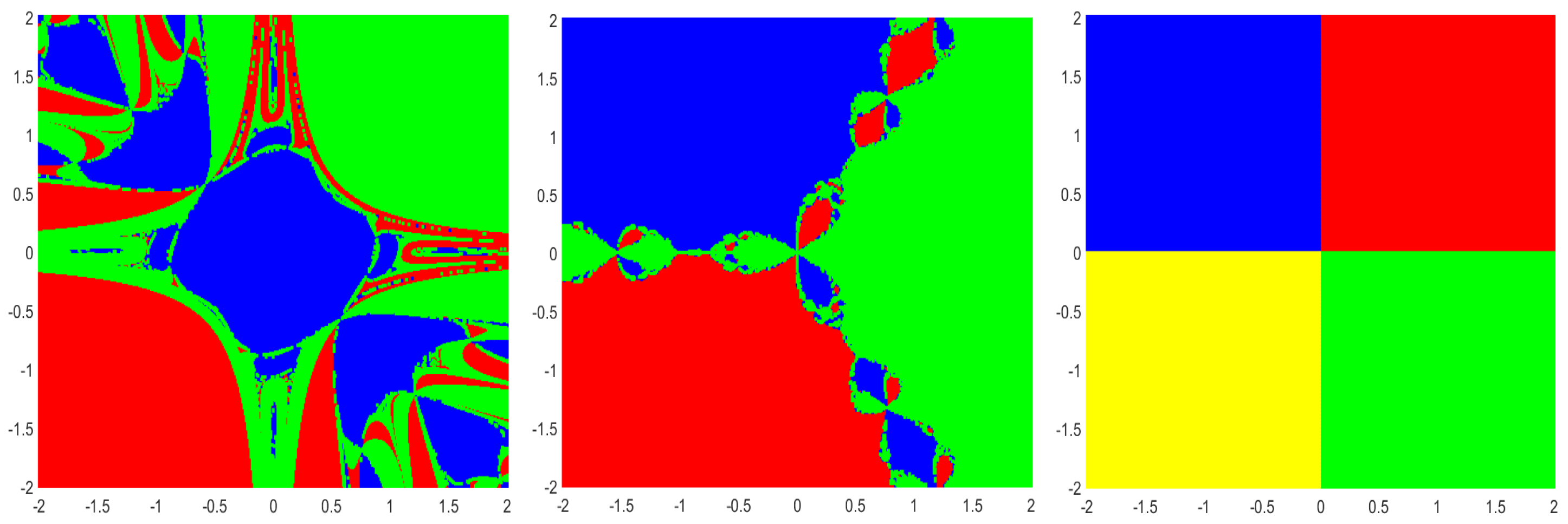
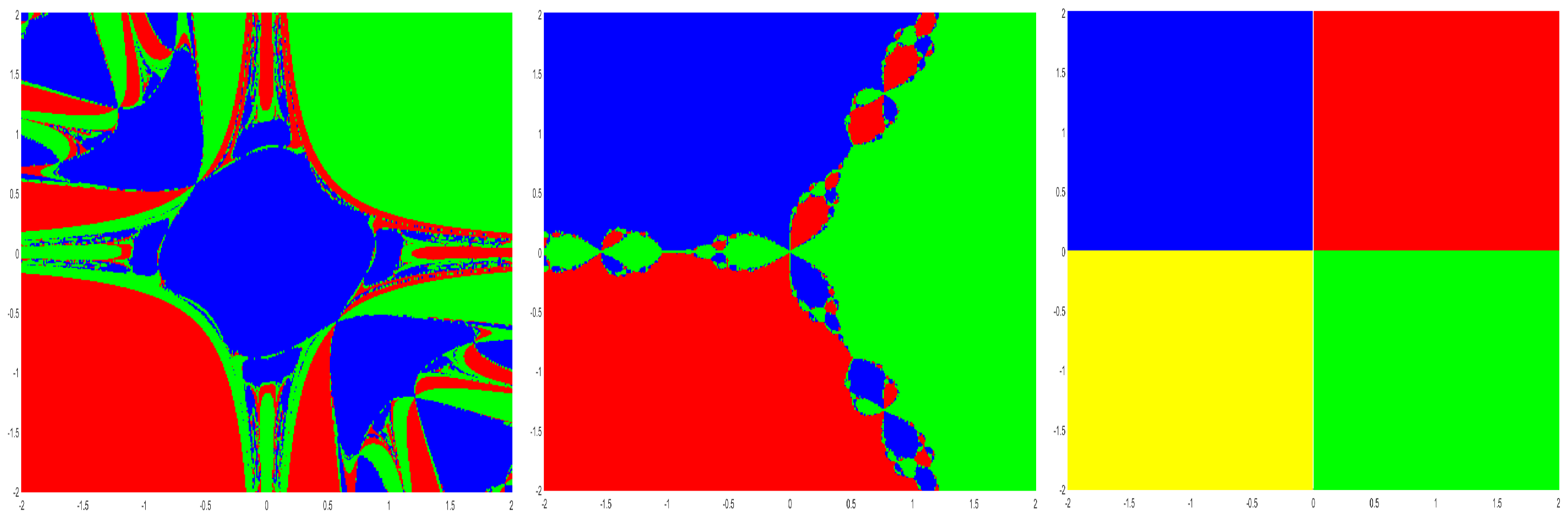
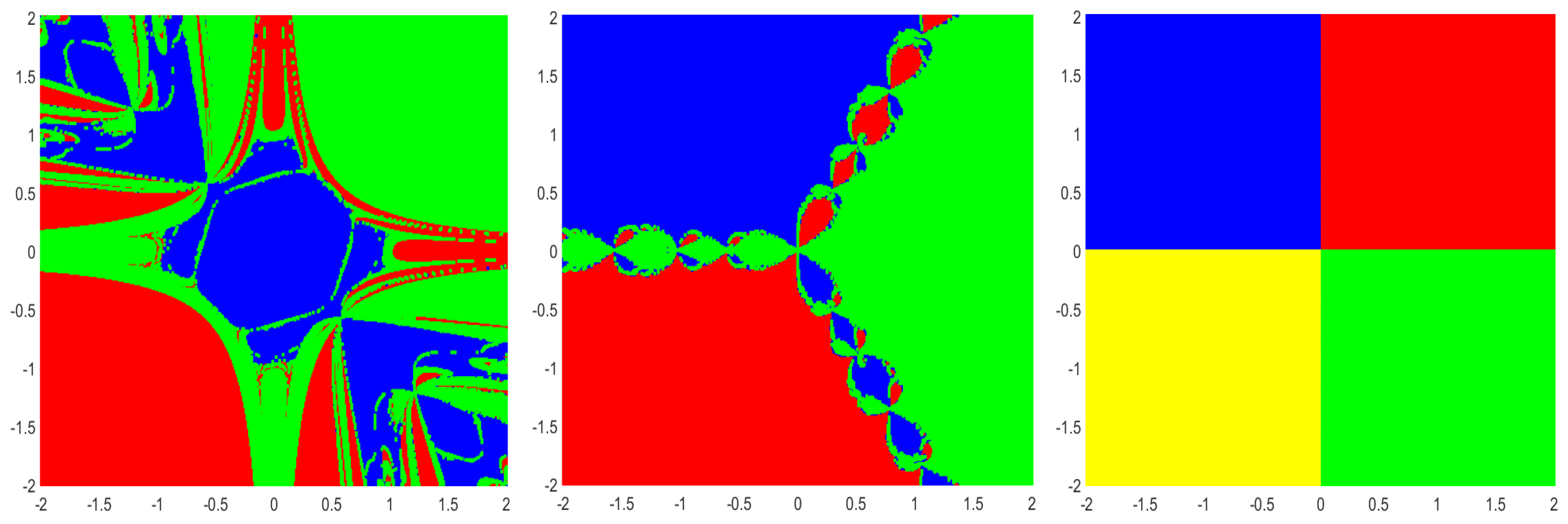
8. Basins of Attraction

In an iterative method, the set of all initial points that lead to convergence towards a solution of an equation is called the basin of attraction [25,26]. Using the approach of basins of attraction, we obtain the area of convergence of the iterative schemes (2), (3), and (4) when applied to the following examples:

Example 5. 

$\left\{\begin{array}{c}{\alpha }^3-\beta =0\hfill \\ {\beta }^3-\alpha =0\hfill \end{array}\right.$ with solutions $\left\{\right(-1,-1),(0,0),(1,1\left)\right\}.$

Example 6. 

$\left\{\begin{array}{c}3{\alpha }^2\beta -{\beta }^3=0\hfill \\ {\alpha }^3-3\alpha {\beta }^2-1=0\hfill \end{array}\right.$ with solutions

$$\{(-{\displaystyle \frac{1}{2}},-{\displaystyle \frac{\sqrt{3}}{2}}),(-{\displaystyle \frac{1}{2}},{\displaystyle \frac{\sqrt{3}}{2}}),(1,0)\}.$$

Example 7. 

$\left\{\begin{array}{c}{\alpha }^2+{\beta }^2-4=0\hfill \\ 3{\alpha }^2+7{\beta }^2-16=0\hfill \end{array}\right.$ with solutions

$$\{(\sqrt{3},1),(-\sqrt{3},1),(\sqrt{3},-1),(-\sqrt{3},-1)\}.$$

Corresponding to the roots of the system of nonlinear equations, the basins of attraction are generated in a rectangle domain $w=\{(\alpha ,\beta )\in {\mathbb{R}}^2:-2\le \alpha \le 2,-2\le \beta \le 2\}$ with equidistant grid points of $401\times 401$. According to the roots, each initial point $({\alpha }_0,{\beta }_0)\in {\mathbb{R}}^2$ is assigned a color, to which the corresponding iterative method converges, starting from $({\alpha }_0,{\beta }_0)$. In the Figure 1, Figure 2 and Figure 3, we assign (a) red to (1, −1), blue to (0, 0) and green to (1, 1) for Example 5, (b) red to $(-{\displaystyle \frac{1}{2}},-{\displaystyle \frac{\sqrt{3}}{2}})$, blue to $(-{\displaystyle \frac{1}{2}},{\displaystyle \frac{\sqrt{3}}{2}})$ and green to (1,0) for Example 6, and (c) red to $(\sqrt{3},1),$ blue to $(-\sqrt{3},1),$ green to $(\sqrt{3},-1)$ and yellow to $(-\sqrt{3},-1)$ in Example 7 respectively. If either the method converges to infinity or it does not converge, then the point is marked black. For a maximum of 100 iterations, a tolerance of ${10}^{-8}$ is used.

9. Conclusions

We studied the Jarrat-type method of convergence order three and two extensions of it with convergence orders six and five, respectively. As mentioned in the introduction, we used assumptions on $A^{\prime }$ and $A^{″}$ only, meaning Methods (2), (3), and (4) can be used to solve problems that are not possible to solve using earlier methods of convergence analysis based on Taylor expansion. We discussed the limitations of our approach and developed new ways to overcome these limitations in Section 5. Finally, we compared the methods with other similar methods using an example. Also, using a basins of attraction approach, the convergence areas of Methods (2), (3), and (4) were given. In future research, our ideas would be extended to other methods to obtain similar benefits [6,7,8,9,10,11,12,14,15,16,17,18,19,20,24,25,26,27,28].

References

1. Ahmad, F.; Tohidi, E.; Ullah, M.Z. Higher order multi-step Jarratt-like method for solving systems of nonlinear equations: Application to PDEs and ODEs. Comput. Math. Appl. 2015, 70, 624–636. [Google Scholar] [CrossRef]
2. Ullah, M.Z.; Serra-Capizzano, S.; Ahmad, F. An efficient multi-step iterative method for computing the numerical solution of systems of nonlinear equations associated with ODEs. Appl. Math. Comput. 2015, 250, 249–259. [Google Scholar] [CrossRef]
3. Argyros, I.K. The Theory and Applications of Iteration Methods; Taylor and Francis Group, CRC Press: Boca Raton, FL, USA, 2022; Volume 2. [Google Scholar]
4. Ullah, M.Z.; Soleymani, F.; Al-Fhaid, A.S. Numerical solution of nonlinear systems by a general class of iterative methods with application to nonlinear PDEs. Numer. Algorithms 2014, 67, 223–242. [Google Scholar] [CrossRef]
5. Yu, J.; Wang, X. A single parameter fourth-order Jarratt type iterative method for solving nonlinear systems. AIMS Math. 2025, 10, 7847–7863. [Google Scholar] [CrossRef]
6. Bartle, R.G. Newton’s method in Banach spaces. Proc. Am. Math. Soc. 1955, 6, 827–831. [Google Scholar]
7. Ben-Israel, A. A Newton-Raphson method for the solution of systems of equations. J. Math. Anal. Appl. 1966, 15, 243–252. [Google Scholar] [CrossRef]
8. Jarratt, P. Some fourth order multipoint iterative methods for solving equations. Math. Comput. 1966, 20, 434–437. [Google Scholar] [CrossRef]
9. Saheya, B.; Chen, G.Q.; Sui, Y.K.; Wu, C.Y. A new Newton-like method for solving nonlinear equations. SpringerPlus 2016, 5, 1269. [Google Scholar] [CrossRef]
10. Ren, H.; Wu, Q.; Bi, W. New variants of Jarratt’s method with sixth-order convergence. Numer. Algorithms 2009, 52, 585–603. [Google Scholar] [CrossRef]
11. Weerakoon, S.; Fernando, T. A variant of Newton’s method with accelerated third-order convergence. Appl. Math. Lett. 2000, 8, 87–93. [Google Scholar] [CrossRef]
12. Petković, M.S.; Neta, B.; Petković, L.D.; Džunić, J. Multipoint methods for solving nonlinear equations: A survey. Appl. Math. Comput. 2014, 226, 635–660. [Google Scholar] [CrossRef]
13. Cordero, A.; Hueso, J.L.; Martínez, E.; Torregrosa, J.R. A modified Newton-Jarratt’s composition. Numer. Algorithms 2010, 55, 87–99. [Google Scholar] [CrossRef]
14. Behl, R.; Cordero, A.; Motsa, S.S.; Torregrosa, J.R. On developing fourth-order optimal families of methods for multiple roots and their dynamics. Appl. Math. Comput. 2015, 265, 520–532. [Google Scholar] [CrossRef]
15. Magreñán, A.A. Different anomalies in a Jarratt family of iterative root finding methods. Appl. Math. Comput. 2014, 233, 29–38. [Google Scholar]
16. Shakhno, S.M.; Iakymchuk, R.P.; Yarmola, H.P. Convergence analysis of a two step method for the nonlinear squares problem with decomposition of operator. J. Numer. Appl. Math. 2018, 128, 82–95. [Google Scholar]
17. Shakhno, S.M.; Gnatyshyn, O.P. On an iterative algorithm of order 1.839… for solving nonlinear operator equations. Appl. Math. Appl. 2005, 161, 253–264. [Google Scholar]
18. Cárdenas, E.; Castro, R.; Sierra, W. A Newton-type midpoint method with high efficiency index. J. Math. Anal. Appl. 2020, 491, 124381. [Google Scholar] [CrossRef]
19. Traub, J.F. Iterative methods for the solution of equations. Am. Math. Soc. 1982, 312. [Google Scholar] [CrossRef]
20. Ostrowski, A.M. Solution of Equations and Systems of Equations: Pure and Applied Mathematics; A Series of Monographs and Textbooks; Elsevier: Amsterdam, The Netherlands, 2016; Volume 9. [Google Scholar]
21. Noor, M.A.; Waseem, M.; Noor, K.I. New iterative technique for solving a system of nonlinear equations. Appl. Math. Comput. 2015, 271, 446–466. [Google Scholar] [CrossRef]
22. Alqahtani, H.F.; Behl, R.; Kansal, M. Higher-Order Iteration Schemes for Solving Nonlinear Systems of Equations. Mathematics 2019, 7, 937. [Google Scholar] [CrossRef]
23. Jayakumar, J. Generalized Simpson-Newton’s Method for Solving Nonlinear Equations with Cubic Convergence. IOSR J. Math. 2013, 7, 58–61. [Google Scholar] [CrossRef]
24. Iliev, A.; Iliev, I. Numerical method with order t for solving system nonlinear equations. Collect. Sci. Work. 2000, 30, 3–4. [Google Scholar]
25. Chun, C.; Lee, M.Y.; Neta, B.; Džunić, J. On optimal fourth-order iterative methods free from second derivative and their dynamics. Appl. Math. Comput. 2012, 218, 6427–6438. [Google Scholar] [CrossRef]
26. Scott, M.; Neta, B.; Chun, C. Basin attractors for various methods. Appl. Math. Comput. 2011, 218, 2584–2599. [Google Scholar] [CrossRef]
27. Ortega, J.M.; Rheinboldt, W.C. Iterative solution of nonlinear equations in several variables. In Classics in Applied Mathematics, Philadelphia: Society for Industrial and Applied Mathematics; Academic Press: Cambridge, MA, USA, 2000; Volume 14. [Google Scholar]
28. Werner, W. Über ein Verfahren der Ordnung 1 + 2 zur Nullstellenbestimmung. Numer. Math. 1979, 32, 333–342. [Google Scholar] [CrossRef]
Figure 1. Dynamical plane of Method (2) with basins of attraction for Example 5 (left), Example 6 (middle), and Example 7 (right).
Axioms 14 00401 g001
Figure 2. Dynamical plane of Method (3) with basins of attraction for Example 5 (left), Example 6 (middle), and Example 7 (right).
Axioms 14 00401 g002
Figure 3. Dynamical plane of Method (4) with basins of attraction for Example 5 (left), Example 6 (middle), and Example 7 (right).
Axioms 14 00401 g003