On the Bivariate Vector-Valued Rational Interpolation and Recovery Problems

Abstract

This paper investigates bivariate vector-valued rational interpolation and recovery problems with common divisors in their denominators. By leveraging these shared divisors and employing a component-wise rational interpolation approach, we reduce the degree of the interpolation problem. Furthermore, a new algorithm for recovering bivariate vector-valued rational functions is proposed. Experimental results demonstrate that, compared to classical algorithms, our method achieves faster computation speed without compromising accuracy. This advantage is particularly evident in the recovery of bivariate vector-valued rational functions.

1. Introduction

The problem of vector-valued rational interpolation is of fundamental importance in computational mathematics, with applications spanning mechanical vibration, data analysis, automatic control, and image processing [1,2,3,4,5]. Building upon our prior work [6] addressing univariate cases with common divisors in their denominators, the framework is extended to the bivariate case.

The classic problem of bivariate vector-valued rational interpolation is generally described as in the following the dataset:

$$\left\{\left((x_i,y_j),{\overrightarrow{V}}_{i,j}\right):(x_i,y_j)\in {\mathbb{R}}^2,{\overrightarrow{V}}_{i,j}=\overrightarrow{V}(x_i,y_j)=\left(v_{i,j,1},\dots ,v_{i,j,s}\right)\in {\mathbb{R}}^s,i=1,\dots ,m,j=1,\dots ,n\right\},$$

where $(x_i,y_j)$ denote the grid point coordinates, ${\overrightarrow{V}}_{i,j}\in {\mathbb{R}}^s$ is the vector-valued function value at $(x_i,y_j)$, and m and n define the number of grid points along the x and y axes, respectively. We construct a bivariate vector-valued rational function

$$\overrightarrow{R}(x,y)={\displaystyle \frac{\overrightarrow{P}(x,y)}{Q(x,y)}},$$

such that

$$\overrightarrow{R}(x_i,y_j)={\displaystyle \frac{\overrightarrow{P}(x_i,y_j)}{Q(x_i,y_j)}}={\overrightarrow{V}}_{i,j},i=1,2,\dots ,m,j=1,2,\dots ,n,$$

where $\overrightarrow{P}(x,y)=(p_1(x,y),p_2(x,y),\dots ,p_s(x,y))$ denotes an s-dimensional vector of bivariate polynomials, and $Q(x,y)$ is a real algebraic polynomial.

Regarding the problem of bivariate vector-valued rational interpolation, Graves-Morris [7,8] and Graves-Morris and Jenkins [9] laid a robust foundation for univariate vector-valued rational interpolation using inverted differences and the Thiele-type continued fraction method, which became pivotal theoretical tools influencing subsequent research on bivariate interpolation. Zhu and Gu [10] extended this to the bivariate case by defining partial inverted differences for vectors via the Samelson inverse transformation. Subsequently, Zhu and Tan [11] presented a matrix algorithm for bivariate vector-valued bifurcated continued fraction interpolation, which broadened the field’s scope. Furthermore, Tan and Tang [12] developed a hybrid method that integrates vector-valued rational and polynomial interpolation.

As described in  [6], the bivariate extension of Thiele-type interpolation inherits the restrictive assumption

$$Q(x,y)\left|\right|\overrightarrow{P}{(x,y)|}^2,$$

where $\left|\overrightarrow{P}(x,y)\right|=\sqrt{p_1{(x,y)}^2+p_2{(x,y)}^2+\dots +p_s{(x,y)}^2}$, significantly limiting its practical utility. Furthermore, the computation of inverted differences may suffer computational instabilities, often necessitating point relocation or component-wise perturbations. These interventions inevitably increase the computational complexity.

To address this methodological gap, we generalize the univariate framework of [6] to bivariate systems by systematically leveraging common factors in the denominators through a component-wise interpolation framework, which enables efficient reduction in computational complexity. Like the univariate approach, we construct a vector-valued rational function by combining multiple scalar-valued rational interpolations as follows:

$$\overrightarrow{R}(x,y)=\left({\displaystyle \frac{p_1(x,y)}{q_1(x,y)}},{\displaystyle \frac{p_2(x,y)}{q_2(x,y)}},\dots ,{\displaystyle \frac{p_s(x,y)}{q_s(x,y)}}\right),$$

(1)

such that

$$\overrightarrow{R}(x_i,y_j)={\overrightarrow{V}}_{i,j},i=1,2,\dots ,m,j=1,2,\dots ,n,$$

where the denominator polynomials $q_k(x,y)$ ($k=1,...,s$) may share non-trivial common divisors, i.e., there exist distinct indices $k_1,k_2\in \{1,...,s\}$ for which $gcd(q_{k_1}(x,y),q_{k_2}(x,y))\ne 1$.

Extending the univariate methodology, we propose a novel bivariate vector-valued rational interpolation algorithm based on Fitzpatrick’s theory. The key innovation involves the systematic exploitation of common factors in the denominators, enabling the following:

• Removal of the constraint $Q(x,y)\left|\right|\overrightarrow{P}{(x,y)|}^2$;
• Bypassing numerically unstable inverted difference computations;
• The utilization of denominators from previously interpolated components to reduce the degree of subsequent interpolation functions, thereby significantly enhancing algorithmic efficiency.

The paper is structured as follows: Section 2 investigates the bivariate vector-valued rational interpolation problem with common factors among vector component denominators. A novel algorithm, leveraging a component-wise approach inspired by scalar rational interpolation, is introduced. This algorithm ingeniously circumvents the uniform denominator constraint of traditional algorithms by exploiting common factors, enabling component-wise interpolation function construction. Section 3 presents a bivariate rational function reconstruction algorithm that is built upon the proposed interpolation framework. This algorithm not only achieves rational reconstruction but also demonstrates symbolic computation utility, as evidenced by its successful application to multivariate polynomial equation systems.

2. Bivariate Vector-Valued Rational Interpolation

This section addresses the interpolation problem for bivariate vector-valued rational functions with non-trivial common divisors in their denominators. Using the multivariate Fitzpatrick algorithm [13] as the theoretical foundation, we develop an extension to bivariate vector-valued rational interpolation. The recursive structure of this algorithm allows for the reuse of denominators from previously interpolated components, thereby reducing the polynomial degrees of subsequent interpolants. Below, we briefly overview its application to bivariate scalar-valued functions.

2.1. Fitzpatrick Algorithm for Bivariate Scalar-Valued Rational Interpolation

Let $\mathbb{K}$ denote a field of characteristic 0, and let $X=(x,y)$. The ring of bivariate polynomials over $\mathbb{K}$ is defined as $\mathcal{P}=\mathbb{K}\left[X\right]=\mathbb{K}[x,y]$. A monomial in $\mathcal{P}$ is of the form $X^{\alpha }=x^{{\alpha }_1}{y}^{{\alpha }_2}$, where $\alpha =({\alpha }_1,{\alpha }_2)\in {\mathbb{N}}^2$ represents the bidegree, and $\left|\alpha \right|={\alpha }_1+{\alpha }_2$ denotes the degree of the monomial. Consider another monomial $X^{\beta }=x^{{\beta }_1}{y}^{{\beta }_2}$ in $\mathcal{P}$, with $\beta =({\beta }_1,{\beta }_2)\in {\mathbb{N}}^2$. The monomial $X^{\alpha }$ is lexicographically less than $X^{\beta }$, denoted $X^{\alpha }{\prec }_{lex}{X}^{\beta }$, if the leftmost non-zero entry of $\beta -\alpha$ is positive.

Now, consider an arbitrary bivariate polynomial $p(x,y)$ in $\mathcal{P}$ expressed as

$$p(x,y)=\sum _{{\alpha }_1=0}^m\sum _{{\alpha }_2=0}^n{c}_{{\alpha }_1,{\alpha }_2}{x}^{{\alpha }_1}{y}^{{\alpha }_2}.$$

The total degree of $p(x,y)$ is defined as $degp(x,y)={max}_{c_{{\alpha }_1,{\alpha }_2}\ne 0}\{{\alpha }_1+{\alpha }_2\}$, the degree with respect to the variable x is defined as ${deg}_{x}p(x,y)={max}_{c_{{\alpha }_1,{\alpha }_2}\ne 0}\left\{{\alpha }_1\right\}$, and the degree with respect to the variable y is defined ${deg}_{y}p(x,y)={max}_{c_{{\alpha }_1,{\alpha }_2}\ne 0}\left\{{\alpha }_2\right\}$.

Next, we introduce the bivariate Cauchy-type rational interpolation on rectangular grid points. Given a dataset of the form

$$\{((x_i,y_j),v_{i,j}):(x_i,y_j)\in {\mathbb{K}}^2,v_{i,j}\in \mathbb{K},i=1,2,\dots ,m,j=1,\dots ,n\},$$

we construct a rational function

$$r(x,y)={\displaystyle \frac{a(x,y)}{b(x,y)}},$$

(2)

such that

$$r(x_i,y_j)={\displaystyle \frac{a(x_i,y_j)}{b(x_i,y_j)}}=v_{i,j},i=1,\dots ,m,j=1,\dots ,n,$$

where $a(x,y),b(x,y)\in \mathcal{P}$ and $b(x_i,y_j)\ne 0$ for all $i,j$. This problem is formally referred to as the bivariate Cauchy-type rational interpolation problem.

It is easy to see that ${\mathcal{P}}^2$ is a free module, with ${\overrightarrow{e}}_1=(1,0)$ and ${\overrightarrow{e}}_2=(0,1)$ as its basis vectors. Let $\overrightarrow{m}=X^{\alpha }·{\overrightarrow{e}}_i$, $i=1,2$ be a monomial in ${\mathcal{P}}^2$.

Definition 1

([13]). For the order ${\prec }_{\xi }$ on ${\mathcal{P}}^2$, the following holds:

 (1)

$X^{\alpha }(1,0){\prec }_{\xi }{X}^{\beta }(1,0)$ if and only if $\left|\alpha \right|<\left|\beta \right|$, or $\left|\alpha \right|=\left|\beta \right|$, and $X^{\alpha }{\prec }_{lex}{X}^{\beta }$;

 (2)

$X^{\alpha }(1,0){\prec }_{\xi }{X}^{\beta }(0,1)$ if and only if $\left|\alpha \right|\le \left|\beta \right|+\xi$;

 (3)

$X^{\alpha }(0,1){\prec }_{\xi }{X}^{\beta }(0,1)$ if and only if $\left|\alpha \right|<\left|\beta \right|$, or $\left|\alpha \right|=\left|\beta \right|$, and $X^{\alpha }{\prec }_{lex}{X}^{\beta }$.

Therein, ξ is a given integer.

Fixing a monomial order ${\prec }_{\xi }$ in ${\mathcal{P}}^2$, each $(a,b)\in {\mathcal{P}}^2$ can be written as a $\mathbb{K}$-linear combination of monomials:

$$(a,b)=\sum _{i=1}^l{c}_i{\overrightarrow{m}}_i,$$

where $c_i\in \mathbb{K}$, $c_i\ne 0$, and ${\overrightarrow{m}}_1{\succ }_{\xi }{\overrightarrow{m}}_2{\succ }_{\xi }\cdots {\succ }_{\xi }{\overrightarrow{m}}_l$. The leading term of $(a,b)$ is defined as $lm(a,b)=c_1{\overrightarrow{m}}_1$. The degree of the rational function $a/b$ is defined as $m_{\xi }(a,b)=max\{dega,degb+\xi \}$.

Let $I_{i,j}=\langle x-x_i,y-y_j\rangle$. It is clearly an ideal in $\mathcal{P}$. If there exist $a(x,y),b(x,y)\in \mathbb{K}[x,y]$ such that

$$a(x,y)-b(x,y)v_{i,j}\equiv 0\mathrm{mod}{I}_{i,j},i=1,\dots ,m,j=1,\dots ,n,$$

then $\left(a\right(x,y),b(x,y\left)\right)$ is called a weak interpolation for (2). Let M denote the set of all weak interpolation defined as

$$M=\left\{(a(x,y),b(x,y))\right|a(x,y)-b(x,y)v_{i,j}\equiv 0\mathrm{mod}{I}_{i,j},i=1,\dots ,m,j=1,\dots ,n\},$$

and it is easily seen that M is a submodule of ${\mathcal{P}}^2$.

We flatten the original 2D interpolation data $((x_i,y_j),v_{i,j})$ (where $i=1,2,\dots ,m,$$j=1,\dots ,n$) into a 1D sequence $(({\overline{x}}_t,{\overline{y}}_t),{\overline{v}}_t)$ with $t=1,\dots ,mn$ while preserving the original grid coordinates $(i,j)$ as metadata. This defines a bijection $\tau :\left[m\right]\times \left[n\right]\to \left[mn\right]$, where $t=\tau (i,j)$, and $(i,j)={\tau }^{-1}\left(t\right)$ (for simplicity, we denote $\left[k\right]=\{1,2,\dots ,k\}$).

Two canonical indexing schemes are presented: Algorithm 1 implements row-major ordering, while Algorithm 2 employs diagonal traversal. We do not exhaustively enumerate all other sorting methods in this work. During data preprocessing, the appropriate sorting method can be selected and defined based on specific needs.   

Algorithm 1: Row traversal indexing.

Algorithm 2: Diagonal traversal indexing.

Thus, the module M composed of weak interpolants for problem (2) can also be represented as follows:

$$M=\{(a(x,y),b(x,y))\mid a(x,y)-b(x,y){\overline{v}}_t\equiv 0\mathrm{mod}{\overline{I}}_t,t=1,\dots ,m·n\},$$

where the ideal ${\overline{I}}_t=\langle x-{\overline{x}}_t,y-{\overline{y}}_t\rangle$. A series of submodules of M is defined as follows:

$$M_k=\{(a(x,y),b(x,y))\mid a(x,y)-b(x,y){\overline{v}}_t\equiv 0\mathrm{mod}{\overline{I}}_t,t=1,\dots ,k\},k=1,\dots ,m·n.$$

Let $M_0={\mathcal{P}}^2$. It is evident that $M_0\supset M_1\supset \cdots \supset M_{m·n}=M$.

Fixing a monomial order ${\prec }_{\xi }$, based on the multivariate Fitzpatrick algorithm in [13], the bivariate case (Algorithm 3) is presented. Given that the Gröbner basis of $M_0$ is $\left\{\right(1,0),(0,1\left)\right\}$, Algorithm 3 can be used to compute the Gröbner basis of the submodules $M_k,k=1,\dots ,m·n$ sequentially.

Algorithm 3: Fitzpatrick algorithm for bivariate scalar rational weak interpolation [13].

If the Gröbner basis of module M is given by

$$\{(a_1(x,y),b_1(x,y)),\dots ,(a_{l_{m·n}}(x,y),b_{l_{m·n}}(x,y))\},$$

then each weak interpolation $\left(a\right(x,y),b(x,y\left)\right)$ in M can be expressed as

$$(a(x,y),b(x,y))=c_1(a_1(x,y),b_1(x,y))+\dots +c_{l_{m·n}}(a_{l_{m·n}}(x,y),b_{l_{m·n}}(x,y)),$$

where the parameters $c_k\in \mathcal{P}$ for $k=1,\dots ,l_{m·n}$. By choosing appropriate $c_k$ such that $b(x_t,y_t)\ne 0$ for $t=1,\dots ,m·n$, we have

$${\displaystyle \frac{a(x,y)}{b(x,y)}}={\displaystyle \frac{c_1{a}_1(x,y)+\dots +c_{l_{m·n}}{a}_{l_{m·n}}(x,y)}{c_1{b}_1(x,y)+\dots +c_{l_{m·n}}{b}_{l_{m·n}}(x,y)}}$$

as a solution to the bivariate Cauchy-type rational interpolation problem.

2.2. Fitzpatrick Algorithm for Bivariate Vector-Valued Rational Interpolation

Next, we discuss the problem of bivariate vector-valued rational interpolation where the denominators of the components share common divisors, i.e., finding a vector-valued rational interpolation function of the form (1).

Similar to the univariate case, classical methods such as the continued fraction method [14,15], the method of solving linear systems of equations [16], or the multivariate Fitzpatrick algorithm [13] are initially employed to compute ${\displaystyle \frac{p_1(x,y)}{q_1(x,y)}}$. Subsequently, the method for solving the components ${\displaystyle \frac{p_k(x,y)}{q_k(x,y)}}$ for $2\le k\le s$ is discussed. The polynomial $q(x,y)$ is selected such that

$$degq(x,y)=\underset{1\le t\le k-1}{max}\{deg{q}_t(x,y)\}.$$

(3)

If there are multiple polynomials that satisfy (3), we choose the one with the largest index.

Assuming that $q(x,y)$ and $q_k(x,y)$ have a greatest common divisor $g_k(x,y)$, then there exist polynomials $s_{k,1}(x,y)$ and $s_{k,2}(x,y)$ such that $q(x,y)=g_k(x,y)·s_{k,1}(x,y)$ and $q_k(x,y)=g_k(x,y)·s_{k,2}(x,y)$. Thus,

$${\displaystyle \frac{p_k(x,y)}{q_k(x,y)}}={\displaystyle \frac{s_{k,1}(x,y)p_k(x,y)}{q(x,y)s_{k,2}(x,y)}}.$$

Let ${\displaystyle \frac{a_k(x,y)}{b_k(x,y)}}={\displaystyle \frac{s_{k,1}(x,y)p_k(x,y)}{s_{k,2}(x,y)}}={\displaystyle \frac{p_k(x,y)}{q_k(x,y)}}q(x,y)$. This leads to a new rational interpolation problem:

$${\displaystyle \frac{a_k(x,y)}{b_k(x,y)}}{|}_{\begin{array}{c}x=x_i\\ y=y_j\end{array}}=v_{i,j,k}q(x_i,y_j),i=1,\dots ,m,j=1,\dots ,n.$$

(4)

For the interpolation problem (4), the module of corresponding weak interpolation is denoted as

$$\widehat{M}=\{(\widehat{a}(x,y),\widehat{b}(x,y))\mid \widehat{a}(x,y)-\widehat{b}(x,y)v_{i,j,k}q(x,y)\equiv 0mod{I}_{i,j},i=1,2,\dots ,m,j=1,2,\dots ,n\},$$

where $I_{i,j}=\langle x-x_i,y-y_j\rangle$. It follows that $(a_k(x,y),b_k(x,y))\in \widehat{M}$. Given that the components ${\displaystyle \frac{p_t(x,y)}{q_t(x,y)}}$ for $t=1,2,\dots ,k-1$ are all rational interpolation functions at the points $(x_i,y_j)$, where $i=1,2,\dots ,m$ and $j=1,2,\dots ,n$, it is required that

$$m_k={deg}_{x}q(x,y)+1\le m,n_k={deg}_{y}q(x,y)+1\le n.$$

(5)

We construct the following polynomials:

$${\omega }_{k,1}\left(x\right)=\prod _{t=1}^{m_k}(x-x_t),{\omega }_{k,2}\left(y\right)=\prod _{t=1}^{n_k}(y-y_t),$$

(6)

$$h_k(x,y)=\sum _{i=1}^{m_k}\sum _{j=1}^{n_k}{v}_{i,j,k}q(x_i,y_j)\prod _{t=1,t\ne i}^{m_k}{\displaystyle \frac{x-x_t}{x_i-x_t}}\prod _{t=1,t\ne j}^{n_k}{\displaystyle \frac{y-y_t}{y_j-y_t}}.$$

(7)

Let ${\xi }_k=deg{h}_k(x,y)$. It can be verified that, under the order ${\prec }_{{\xi }_k}$, the set $\{(h_k(x,y),1),({\omega }_{k,1}\left(x\right),0),({\omega }_{k,2}\left(y\right),0)\}$ constitutes a Gröbner basis for the module

$${\widehat{M}}_{k,m_k,n_k}=\left\{(\tilde{a}(x,y),\tilde{b}(x,y))\mid \tilde{a}(x,y)-\tilde{b}(x,y)v_{i,j,k}q(x,y)\equiv 0mod{I}_{i,j},i=1,\dots ,m_k,j=1,\dots ,n_k\right\}.$$

Consequently, for $(a_k(x,y),b_k(x,y))\in \widehat{M}\subset {\widehat{M}}_{k,m_k,n_k}$, there exist polynomials $c_{k,1}(x,y)$, $c_{k,2}(x,y)$, and $c_{k,3}(x,y)\in \mathbb{K}[x,y]$ such that

$$(a_k(x,y),b_k(x,y))=c_{k,1}(x,y)·({\omega }_{k,1}\left(x\right),0)+c_{k,2}(x,y)·({\omega }_{k,2}\left(y\right),0)+c_{k,3}(x,y)·(h_k(x,y),1).$$

Given that $(a_k(x,y),b_k(x,y))\in \widehat{M}$, it follows that, for $i=1,\dots ,m$ and $j=1,\dots ,n$, if $c_{k,3}(x_i,y_j)\ne 0$, then

$$\begin{array}{cc}\hfill & {\displaystyle \frac{c_{k,1}(x_i,y_j){\omega }_{k,1}\left(x_i\right)+c_{k,2}(x_i,y_j){\omega }_{k,2}\left(y_j\right)+c_{k,3}(x_i,y_j)h_k(x_i,y_j)}{c_{k,3}(x_i,y_j)·1}}={\displaystyle \frac{a_k(x_i,y_j)}{b_k(x_i,y_j)}}=v_{i,j,k}q(x_i,y_j),\hfill \\ \hfill & i=1,2,\dots ,m,j=1,2,\dots ,n.\hfill \end{array}$$

Considering the definitions of ${\omega }_{k,1}(x,y)$ and ${\omega }_{k,2}(x,y)$, the above equation holds for $1\le i\le m_k$ and $1\le j\le n_k$, irrespective of the values of $c_{k,1}(x,y)$, $c_{k,2}(x,y)$, and $c_{k,3}(x,y)$. Therefore, we only need to solve for $c_{k,1}(x,y)$, $c_{k,2}(x,y)$, and $c_{k,3}(x,y)$ under the following cases:

When $m_k<m$ and $n_k\le n$, the following equation holds:

$$w_{i,j,k}:={\displaystyle \frac{c_{k,1}(x,y)}{c_{k,3}(x,y)}}{|}_{\begin{array}{c}x=x_i\\ y=y_j\end{array}}={\displaystyle \frac{v_{i,j,k}q(x_i,y_j)-h_k(x_i,y_j)}{{\omega }_{k,1}\left(x_i\right)}},i=m_k+1,\dots ,m,j=1,\dots ,n_k.$$

(8)

When $m_k\le m$ and $n_k<n$, the following equation holds:

$$u_{i,j,k}:={\displaystyle \frac{c_{k,2}(x,y)}{c_{k,3}(x,y)}}{|}_{\begin{array}{c}x=x_i\\ y=y_j\end{array}}={\displaystyle \frac{v_{i,j,k}q(x_i,y_j)-h_k(x_i,y_j)}{{\omega }_{k,2}\left(y_j\right)}},i=1,\dots ,m_k,j=n_k+1,\dots ,n.$$

(9)

When $m_k<m$ and $n_k<n$, the following equation holds:

$$\begin{array}{cc}\hfill g_{i,j,k}& :={\displaystyle \frac{c_{k,1}(x_i,y_j){\omega }_{k,1}\left(x_i\right)+c_{k,2}(x_i,y_j){\omega }_{k,2}\left(y_j\right)}{c_{k,3}(x_i,y_j)}}\hfill \\ \hfill & =v_{i,j,k}q(x_i,y_j)-h_k(x_i,y_j),i=m_k+1,\dots ,m,j=n_k+1,\dots ,n.\hfill \end{array}$$

(10)

Based on the different values of $m_k$ and $n_k$, we discuss the solution of $c_{k,1}(x,y)$, $c_{k,2}(x,y)$, and $c_{k,3}(x,y)$ in the following cases:

(1) When $m_k<m$ and $n_k<n$, let $N=m_k(n-n_k)+n_k(m-m_k)+(n-n_k)(m-m_k)+1$. Define the index set E as the collection of all ordered pairs $({\alpha }_t,{\beta }_t)$ arranged in ascending lexicographical order. Given positive integers $r_1,r_2,r_3$ such that $r_1+r_2+r_3=N$, we construct the following polynomials by taking the first $r_1,r_2$, and $r_3$ elements from E as exponents:

$$c_{k,1}(x,y)=\sum _{k_1=1}^{r_1}{d}_{k_1}{x}^{{\alpha }_{k_1}}{y}^{{\beta }_{k_1}},c_{k,2}(x,y)=\sum _{k_2=1}^{r_2}{e}_{k_2}{x}^{{\alpha }_{k_2}}{y}^{{\beta }_{k_2}},c_{k,3}(x,y)=\sum _{k_3=1}^{r_3}{f}_{k_3}{x}^{{\alpha }_{k_3}}{y}^{{\beta }_{k_3}}.$$

(11)

Next, we substitute the polynomials into the linear rational interpolation system (12), which is derived from Equations (8)–(10):

$$\left\{\begin{array}{cc}\hfill & {\displaystyle \frac{c_{k,2}(x_i,y_j)}{c_{k,3}(x_i,y_j)}}=u_{i,j,k},i=1,\dots ,m_k,j=n_k+1,\dots ,n,\hfill \\ \hfill & {\displaystyle \frac{c_{k,1}(x_i,y_j)}{c_{k,3}(x_i,y_j)}}=w_{i,j,k},i=m_k+1,\dots ,m,j=1,\dots ,n_k,\hfill \\ \hfill & {\displaystyle \frac{c_{k,1}(x_i,y_j){\omega }_{k,1}\left(x_i\right)+c_{k,2}(x_i,y_j){\omega }_{k,2}\left(y_j\right)}{c_{k,3}(x_i,y_j)}}=g_{i,j,k},i=m_k+1,\dots ,m,j=n_k+1,\dots ,n.\hfill \end{array}\right.$$

(12)

This system forms a set of equations with respect to the undetermined coefficients $d_{k_1}$ for $k_1=1,2,\dots ,r_1$, $e_{k_2}$ for $k_2=1,2,\dots ,r_2$, and $f_{k_3}$ for $k_3=1,2,\dots ,r_3$:

$$\left\{\begin{array}{cc}\hfill & \sum _{k_2=1}^{r_2}{e}_{k_2}{x}_i^{{\alpha }_{k_2}}{y}_j^{{\beta }_{k_2}}-u_{i,j,k}·\sum _{k_3=1}^{r_3}{f}_{k_3}{x}_i^{{\alpha }_{k_3}}{y}_j^{{\beta }_{k_3}}=0,i=1,\dots ,m_k,j=n_k+1,\dots ,n,\hfill \\ \hfill & \sum _{k_1=1}^{r_1}{d}_{k_1}{x}_i^{{\alpha }_{k_1}}{y}_j^{{\beta }_{k_1}}-w_{i,j,k}·\sum _{k_3=1}^{r_3}{f}_{k_3}{x}_i^{{\alpha }_{k_3}}{y}_j^{{\beta }_{k_3}}=0,i=m_k+1,\dots ,m,j=1,\dots ,n_k,\hfill \\ \hfill & \sum _{k_1=1}^{r_1}{d}_{k_1}{x}_i^{{\alpha }_{k_1}}{y}_j^{{\beta }_{k_1}}{\omega }_{k,1}\left(x_i\right)+\sum _{k_2=1}^{r_2}{e}_{k_2}{x}_i^{{\alpha }_{k_2}}{y}_j^{{\beta }_{k_2}}{\omega }_{k,2}\left(y_j\right)-g_{i,j,k}·\sum _{k_3=1}^{r_3}{f}_{k_3}{x}_i^{{\alpha }_{k_3}}{y}_j^{{\beta }_{k_3}}=0,\hfill \\ \hfill & i=m_k+1,\dots ,m,j=n_k+1,\dots ,n.\hfill \end{array}\right.$$

Solving this system for the polynomial coefficients $d_{k_1},e_{k_2},$ and $f_{k_3}$, we ensure that $c_{k,3}(x_i,y_j)\ne 0$ for all $i=1,\dots ,m$ and $j=1,\dots ,n$. Substituting the obtained coefficients back into Equation (11), we determine the specific forms of $c_{k,1}(x,y)$, $c_{k,2}(x,y)$, and $c_{k,3}(x,y)$.

(2) When $m_k=m$ and $n_k<n$, set ${\displaystyle \frac{c_{k,1}}{c_{k,3}}}=0$ and only compute ${\displaystyle \frac{c_{k,2}}{c_{k,3}}}$ to satisfy (9).

(3) When $m_k<m$ and $n_k=n$, set ${\displaystyle \frac{c_{k,2}}{c_{k,3}}}=0$ and only compute ${\displaystyle \frac{c_{k,1}}{c_{k,3}}}$ to satisfy (8).

(4) When both $m_k=m$ and $n_k=n$ hold, set $c_{k,1}=0$, $c_{k,2}=0$, and $c_{k,3}=1$.

Once $c_{k,1}(x,y)$, $c_{k,2}(x,y)$, and $c_{k,3}(x,y)$ are determined, the expression becomes

$${\displaystyle \frac{p_k(x,y)}{q(x,y)}}={\displaystyle \frac{c_{k,1}(x,y){\omega }_{k,1}\left(x\right)+c_{k,2}(x,y){\omega }_{k,2}\left(y\right)+c_{k,3}(x,y)h_k(x,y)}{c_{k,3}(x,y)·q(x,y)}}.$$

Based on this, the bivariate Fitzpatrick-type vector-valued rational interpolation algorithm is presented (see Algorithm 4).

Next, we compare our algorithm with the classical vector-valued rational interpolation algorithm in two aspects: the degree of the interpolation results and the approximation effectiveness. Since most bivariate vector-valued rational interpolation algorithms are built upon the theory of bivariate Thiele-type vector-valued rational interpolation  [10,15], we have chosen to compare our method specifically with the Thiele-type algorithm.

Due to the complexity involved in calculating the extrema of bivariate functions, we compute the error in the following manner: Let the interpolation function be denoted as $\overrightarrow{R}(x,y)=\left(r_1(x,y),r_2(x,y),\dots ,r_s(x,y)\right)$ and the original function as $\overrightarrow{V}(x,y)=\left(v_1(x,y),v_2(x,y),\dots ,v_s(x,y)\right)$. The error for the k-th component is then given by

$$e_k(x,y)=r_k(x,y)-v_k(x,y),k=1,2,\dots ,s.$$

Consequently, the error vector for the interpolation is

$$\overrightarrow{E}(x,y)=\left(e_1(x,y),e_2(x,y),\dots ,e_s(x,y)\right).$$

To systematically evaluate the approximation accuracy, we construct an evaluation grid $T=\{(x_i,y_j):i=0,1,\dots ,\overline{m},j=0,1,\dots ,\overline{n}\}$ by uniformly dividing the x domain into $\overline{m}$ subintervals and the y domain into $\overline{n}$ subintervals, where $\overline{m}$ and $\overline{n}$ denote the number of sample points along each axis.The global error bound is then computed as

$$ERR=\underset{1\le k\le s}{max}{E}_k,$$

(13)

where $E_k={max}_{(x_i,y_j)\in T}\left|e_k(x_i,y_j)\right|$ for $k=1,2,\dots ,s$ represents the error bound for the k-th component.

Example 1.

Given the vector function $\left({\displaystyle \frac{\sqrt{y}}{x+y}},{\displaystyle \frac{\sqrt{x}}{y(x+y)}}\right)$ with its data at the points $(x_i,y_j)$, as shown in

Table 1. Interpolation data.

		${\mathit{x}}_{\mathit{i}}$	${\mathit{x}}_1=1$	${\mathit{x}}_2=4$	${\mathit{x}}_3=9$	${\mathit{x}}_4=16$
	${\overrightarrow{\mathit{V}}}_{\mathit{i},\mathit{j}}$
${\mathit{y}}_{\mathit{j}}$
$y_1=1$			$\left({\displaystyle \frac{1}{2}},{\displaystyle \frac{1}{2}}\right)$	$\left({\displaystyle \frac{1}{5}},{\displaystyle \frac{2}{5}}\right)$	$\left({\displaystyle \frac{1}{10}},{\displaystyle \frac{3}{10}}\right)$	$\left({\displaystyle \frac{1}{17}},{\displaystyle \frac{4}{17}}\right)$
$y_2=4$			$\left({\displaystyle \frac{2}{5}},{\displaystyle \frac{1}{20}}\right)$	$\left({\displaystyle \frac{1}{4}},{\displaystyle \frac{1}{16}}\right)$	$\left({\displaystyle \frac{2}{13}},{\displaystyle \frac{3}{52}}\right)$	$\left({\displaystyle \frac{1}{10}},{\displaystyle \frac{1}{20}}\right)$
$y_3=9$			$\left({\displaystyle \frac{3}{10}},{\displaystyle \frac{1}{90}}\right)$	$\left({\displaystyle \frac{3}{13}},{\displaystyle \frac{2}{117}}\right)$	$\left({\displaystyle \frac{1}{6}},{\displaystyle \frac{1}{54}}\right)$	$\left({\displaystyle \frac{3}{25}},{\displaystyle \frac{4}{225}}\right)$

, we seek a vector-valued rational interpolation function that satisfies the data in the table.    

Algorithm 4: Fitzpatrick algorithm for bivariate vector-valued rational interpolation.

Using Algorithm  4, the interpolation result is

$$\left(-{\displaystyle \frac{1}{60}}·{\displaystyle \frac{y^2-25y-36}{x+y}},{\displaystyle \frac{1}{1260}}·{\displaystyle \frac{x^3-35x^2+574x+720}{y(x+y)}}\right).$$

Applying the bivariate Thiele-type vector-valued rational interpolation method ($BVR{I}_x$ type) [10, 15] results in a rational function with numerator and denominator degrees of 11 and 10, respectively (see Appendix A for details).

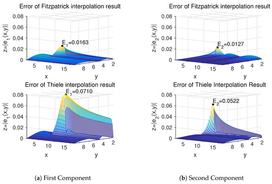
Under the conditions $\overline{m}=75$ and $\overline{n}=40$, using Formula (13) to evaluate the algorithm error, the error bound for Algorithm 4 is 0.0163, whereas the error bound for the bivariate Thiele-type algorithm is 0.0710. Figure 1 demonstrates that, for this particular problem, the bivariate Fitzpatrick-type algorithm outperforms the bivariate Thiele-type algorithm in terms of the component-wise error, showing significantly smaller deviations from the original function.

Example 2.

For the vector functions ${\overrightarrow{V}}_i\left(x\right)$ listed in

Table 2. Vector functions and knots.

i	${\overrightarrow{\mathit{V}}}_{\mathit{i}}(\mathit{x},\mathit{y})$	Knots of x	Knots of y
1	$\left(ln(x+y),e^{xy}\right)$	0.2:0.2:1.4	0.2:0.2:1.4
2	$\left(cos\left({\displaystyle \frac{x+y}{5}}\right),sin\left({\displaystyle \frac{xy}{25}}\right)\right)$	0.5:0.5:3.5	0.5:0.5:3.5
3	$\left({\displaystyle \frac{\sqrt[3]{xy}}{x+y}},{\displaystyle \frac{\sqrt{xy}}{x+y}},{\displaystyle \frac{xy}{x+y}}\right)$	1.0:1.0:7.0	1.0:1.0:7.0
4	$\left(cos\left(x^{2}y\right),sin\left(x{y}^2\right),sin\left(x\right)cos\left(y\right)\right)$	0.1:0.1:0.7	0.1:0.1:0.7
5	$\left({\displaystyle \frac{ln(x+y)}{x+y}},{\displaystyle \frac{x+y}{x^2+y^2}},{\displaystyle \frac{ln\left(xy\right)}{x+y}},{\displaystyle \frac{xy}{{(x+y)}^2}}\right)$	2.0:2.0:14.0	2.0:2.0:14.0
6	$\left(cos(x+y),sin\left(x\right)+cos\left(y\right),sin\left(xy\right),sin\left(x\right)cos\left(y\right)\right)$	0.2:0.2:1.4	0.2:0.2:1.4
7	$\left({\displaystyle \frac{\sqrt{xy}}{x+y}},cos\left({\displaystyle \frac{1}{4}}xy\right),{\displaystyle \frac{e^{\sqrt{x^2+y}}}{x+y}},sin\left({\displaystyle \frac{1}{4}}xy\right),{\displaystyle \frac{ln(x^2+y)}{x+y}}\right)$	0.4:0.2:1.6	0.4:0.2:1.6
8	$\left({\displaystyle \frac{\sqrt{y}}{x^2+y^2}},{\displaystyle \frac{y}{x(x^2+y^2)}},{\displaystyle \frac{\sqrt{x+y}}{x^2+y^2}},{\displaystyle \frac{x}{y(x^2+y^2)}},{\displaystyle \frac{\sqrt{x}}{x^2+y^2}}\right)$	2.0:2.0:14.0	3.0:2.0:15.0
9	$\left({\displaystyle \frac{cos(x-y)}{x+y}},ln(x+y),e^{xy},{\displaystyle \frac{sin(x-y)}{x+y}},tan(x-y),\sqrt{x(x+y)}\right)$	0.3:0.2:1.5	0.2:0.2:1.4
10	$\left({\displaystyle \frac{\sqrt{xy}}{x^2-y^2}},{\displaystyle \frac{\sqrt{y}}{{(x+y)}^2}},{\displaystyle \frac{x-y}{y(x+y)}},{\displaystyle \frac{xy}{x^2-y^2}},{\displaystyle \frac{x}{y(x+y)}},{\displaystyle \frac{\sqrt{x}}{{(x+y)}^2}}\right)$	2.0:2.0:14.0	3.0:2.0:15.0

, data samples were utilized as specified ($a:h:b$ denotes a row vector starting at a, ending at b, with a step size of h). We then applied both Algorithm 4 and the bivariate Thiele-type vector-valued rational interpolation algorithm, aiming to compare their approximation performance and computation times.

Let $\overline{m}=\overline{n}=10$. The error bounds for Algorithm 4 and the bivariate Thiele-type interpolation algorithm are computed using Formula (13). These bounds are reported in the 2nd and 3rd columns of

Table 3. Comparison of errors and runtime between the results of two algorithms.

${\overrightarrow{\mathit{V}}}_{\mathit{i}}(\mathit{x},\mathit{y})$	$\mathbf{ERR}$			Runtime
	Algorithm 4	Thiele		Algorithm 4	Thiele
${\overrightarrow{V}}_1(x,y)$	$7.2083193\times {10}^{-2}$	$1.21009658\times {10}^1$		0.422	4.453
${\overrightarrow{V}}_2(x,y)$	$7.493208\times {10}^{-4}$	$5.16361639\times {10}^{-2}$		0.407	6.125
${\overrightarrow{V}}_3(x,y)$	$3.6820\times {10}^{-5}$	$1.50595\times {10}^{-4}$		0.500	15.313
${\overrightarrow{V}}_4(x,y)$	$4.837601537\times {10}^{-1}$	$1.533681465\times {10}^2$		0.469	30.875
${\overrightarrow{V}}_5(x,y)$	$2.951622794\times {10}^{-2}$	$1.557168816\times {10}^1$		0.515	31.156
${\overrightarrow{V}}_6(x,y)$	$4.78932192\times {10}^{-2}$	$4.912879374\times {10}^1$		0.563	58.719
${\overrightarrow{V}}_7(x,y)$	$2.45816231\times {10}^{-2}$	$2.32381466\times {10}^{-1}$		0.641	89.016
${\overrightarrow{V}}_8(x,y)$	$1.168715808\times {10}^{-2}$	$1.564390811\times {10}^0$		0.672	76.797
${\overrightarrow{V}}_9(x,y)$	$8.392071917\times {10}^{-1}$	$2.441074888\times {10}^3$		0.813	124.172
${\overrightarrow{V}}_{10}(x,y)$	$4.2300120\times {10}^{-2}$	$1.158196203\times {10}^{-1}$		0.828	124.953

, respectively. The runtimes are listed in the 4th and 5th columns. Table 3 shows that as the dimensionality of the function increased, Algorithm 4 significantly outperformed the bivariate Thiele-type algorithm in computation time, with the gap between them widening progressively. Additionally, Algorithm 4 has a lower interpolation error bound than the bivariate Thiele-type algorithm.

Remark 1.

All computations were performed on a Lenovo laptop with an Intel Core i7-8565U processor (Intel, Santa Clara, CA, USA), 8 GB RAM, and Windows 10 Enterprise Edition. Maple 2016 software was utilized for both computation and analysis.

3. Bivariate Vector-Valued Rational Recovery

In this section, we explore a crucial application of bivariate vector-valued rational interpolation: the reconstruction of unknown bivariate vector-valued rational functions. Consider an unknown function

$$\overrightarrow{V}(x,y)=(v_1(x,y),v_2(x,y),\cdots ,v_s(x,y)),$$

accessible via a black box $B:{\mathbb{R}}^2\to {\mathbb{R}}^s$. For any input $(x_i,y_j)\in {\mathbb{R}}^2$, the black box B returns $\overrightarrow{V}(x_i,y_j)=(v_1(x_i,y_j),v_2(x_i,y_j),\cdots ,v_s(x_i,y_j))\in {\mathbb{R}}^s$. Next, we explore an effective interpolation method to reconstruct the unknown bivariate vector-valued rational function $\overrightarrow{V}(x,y)$. To begin with, we acquire sufficient data via the black box:

$$\left\{\left((x_i,y_j),{\overrightarrow{V}}_{i,j}\right):(x_i,y_j)\in {\mathbb{R}}^2,{\overrightarrow{V}}_{i,j}=\overrightarrow{V}(x_i,y_j)=\left(v_{i,j,1},\dots ,v_{i,j,s}\right)\in {\mathbb{R}}^s,i=1,\dots ,M,j=1,\dots ,N\right\}.$$

Then, we select $m<M$ and $n<N$ to form a subset of these points:

$$\left\{\left((x_i,y_j),{\overrightarrow{V}}_{i,j}\right):i=1,\dots ,m,j=1,\dots ,n\right\}.$$

Using this subset, we aim to reconstruct a vector-valued rational function

$$\overrightarrow{R}(x,y)=\left({\displaystyle \frac{p_1(x,y)}{q_1(x,y)}},{\displaystyle \frac{p_2(x,y)}{q_2(x,y)}},\dots ,{\displaystyle \frac{p_s(x,y)}{q_s(x,y)}}\right),$$

such that

$$\overrightarrow{R}(x_i,y_j)=\overrightarrow{V}(x_i,y_j),i=1,\dots ,M,j=1,\dots ,N,$$

where $deg{p}_i\le l$ and $deg{q}_i\le d$ for all $1\le i\le s$, with $l<M$ and $d<N$. In this case, we consider $\overrightarrow{R}(x,y)$ to be the function obtained by recovering $\overrightarrow{V}(x,y)$.

In the algorithm design, a sequential component recovery strategy is used. To reconstruct the first rational component ${\displaystyle \frac{p_1(x,y)}{q_1(x,y)}}$, we sample the component $v_1(x,y)$ of the black box function at two distinct sets of points:

• Computation set $J_1=\{({\overline{x}}_i,{\overline{y}}_i):i=1,2,\cdots ,t\}$, with adjustable parameter t;
• Validation set $J_2=\{({\tilde{x}}_i,{\tilde{y}}_i):i=1,2\}$, where ${\tilde{x}}_i$ and ${\tilde{y}}_i$ ($i=1,2$) are sufficiently large prime numbers.

The rational function $r_t^{\left(1\right)}(x,y)$ is first constructed over $J_1$ using interpolation. Its validity is then tested on $J_2$: If $r_t^{\left(1\right)}({\tilde{x}}_i,{\tilde{y}}_i)=v_1({\tilde{x}}_i,{\tilde{y}}_i)$ holds for both $i=1,2$, we accept ${\displaystyle \frac{p_1(x,y)}{q_1(x,y)}}=r_t^{\left(1\right)}(x,y)$; otherwise, we increment t by 1, compute the updated function $r_{t+1}^{\left(1\right)}(x,y)$ based on the previous $r_t^{\left(1\right)}(x,y)$, and iterate until validation succeeds.

Next, the second component is recovered. First, let $q(x,y)=q_1(x,y)$, $m_2={deg}_{x}q(x,y)+1$, and $n_2={deg}_{y}q(x,y)+1$. If $degq(x,y)=0$, then the recovery method for ${\displaystyle \frac{p_2(x,y)}{q_2(x,y)}}$ follows the same procedure as for ${\displaystyle \frac{p_1(x,y)}{q_1(x,y)}}$. For $degq(x,y)>0$, two methods are available:

Method 1: The values $v_{i,j,2}$ are sampled from the black box component $v_2(x,y)$, where the indices $(i,j)$ belong to the set $\left[m\right]\times \left[n\right]\setminus \left[m_2\right]\times \left[n_2\right]$. The parameters m and n are selected to satisfy $m_2<m<M$ and $n_2<n<N$. Applying the method of undetermined coefficients, we derive the linear rational interpolation system:

$$\left\{\begin{array}{ccc}\hfill & {\displaystyle \frac{c_{2,2}(x_i,y_j)}{c_{2,3}(x_i,y_j)}}=u_{i,j,2},\hfill & \hfill i=1,\dots ,m_2,j=n_2+1,\dots ,n\left(\mathrm{a}\right),\\ \hfill & {\displaystyle \frac{c_{2,1}(x_i,y_j)}{c_{2,3}(x_i,y_j)}}=w_{i,j,2},\hfill & \hfill i=m_2+1,\dots ,m,j=1,\dots ,n_2\left(\mathrm{b}\right),\\ \hfill & {\displaystyle \frac{c_{2,1}(x_i,y_j){\omega }_{2,1}\left(x_i\right)+c_{2,2}(x_i,y_j){\omega }_{2,2}\left(y_j\right)}{c_{2,3}(x_i,y_j)}}=g_{i,j,2},\hfill & \hfill i=m_2+1,\dots ,m,j=n_2+1,\dots ,n\left(\mathrm{c}\right).\end{array}\right.$$

Solving this system yields the coefficients $c_{2,1}(x,y)$, $c_{2,2}(x,y)$, and $c_{2,3}(x,y)$. We then compute

$$r_1^{\left(2\right)}(x,y)={\displaystyle \frac{c_{2,1}(x,y){\omega }_{2,1}\left(x\right)+c_{2,2}(x,y){\omega }_{2,2}\left(y\right)+c_{2,3}(x,y)h_2(x,y)}{c_{2,3}(x,y)·q(x,y)}}.$$

The validation set $J_2=\{({\tilde{x}}_i,{\tilde{y}}_i)\mid i=1,2\}$ is used to test the recovery of this rational component. If validation fails, m and n are incremented to include additional interpolation points. This process iterates until the t-th iteration produces an interpolant $r_t^{\left(2\right)}(x,y)$ satisfying the verification criteria, at which point we set ${\displaystyle \frac{p_2(x,y)}{q_2(x,y)}}=r_t^{\left(2\right)}(x,y)$. Based on the previous discussion of interpolation problems in this work, the existence of a solution is ensured provided there are sufficient interpolation points.

Method 2: When the condition ${deg}_y{c}_{2,1}(x,y)+{deg}_y{c}_{2,3}(x,y)<n_2$ is satisfied, formula (b) is applied as follows:

$${\displaystyle \frac{c_{2,1}(x,y)}{c_{2,3}(x,y)}}=w_{i,j,2},i=m_2+1,\dots ,m,j=1,\dots ,n_2.$$

By selecting a sufficiently large M and utilizing interpolation data $\{(x_i,y_j),w_{i,j,2}\}$ with $i=m_2+1,\dots ,M$ and $j=1,\dots ,n_2$, the identical procedure employed for reconstructing ${\displaystyle \frac{q_1(x,y)}{p_1(x,y)}}$ is applied to recover the rational component ${\displaystyle \frac{c_{2,3}(x,y)}{c_{2,1}(x,y)}}$, ensuring consistency with function values at corresponding points.

Analogously, when ${deg}_x{c}_{2,2}(x,y)+{deg}_x{c}_{2,3}(x,y)<m_2$, formula (a) is employed:

$${\displaystyle \frac{c_{2,2}(x,y)}{c_{2,3}(x,y)}}=u_{i,j,2},i=1,\dots ,m_2,j=n_2+1,\dots ,n.$$

With a sufficiently large N, interpolation data $\{(x_i,y_j),u_{i,j,2}\}$ ($i=1,\dots ,m_2$, $j=n_2+1,\dots ,N$) are used to recover ${\displaystyle \frac{c_{2,3}(x,y)}{c_{2,2}(x,y)}}$, matching function values at respective points.

• Critical Implementation Details:

• For recovering ${\displaystyle \frac{c_{2,3}(x,y)}{c_{2,1}(x,y)}}$ via formula (b), the validation points must have ordinates from $\{y_1,\dots ,y_{n_2}\}$. Thus, points with sufficiently large prime abscissas and $y_j$ ($j=1,\dots ,n_2$) as ordinates are selected.
• For recovering ${\displaystyle \frac{c_{2,3}(x,y)}{c_{2,2}(x,y)}}$ via formula (a), the validation points are chosen with abscissas from $\{x_1,\dots ,x_{m_2}\}$ and sufficiently large prime ordinates.

After recovering low-degree rational functions ${\displaystyle \frac{c_{2,3}(x,y)}{c_{2,1}(x,y)}}$ and ${\displaystyle \frac{c_{2,3}(x,y)}{c_{2,2}(x,y)}}$ via Method 2, if their denominators differ, we reconcile them by computing the least common multiple (LCM). Specifically, given rational functions ${\displaystyle \frac{{\tilde{c}}_{2,1}(x,y)}{{\tilde{c}}_{2,3}(x,y)}}$ and ${\displaystyle \frac{{\tilde{c}}_{2,2}(x,y)}{{\tilde{\tilde{c}}}_{2,3}(x,y)}}$, the unified denominator is $c_{2,3}(x,y)=\mathrm{lcm}({\tilde{c}}_{2,3}(x,y),{\tilde{\tilde{c}}}_{2,3}(x,y))$, resulting in ${\displaystyle \frac{c_{2,1}(x,y)}{c_{2,3}(x,y)}}={\displaystyle \frac{{\tilde{c}}_{2,1}(x,y)}{{\tilde{c}}_{2,3}(x,y)}}$ and ${\displaystyle \frac{c_{2,2}(x,y)}{c_{2,3}(x,y)}}={\displaystyle \frac{{\tilde{\tilde{c}}}_{2,2}(x,y)}{{\tilde{\tilde{c}}}_{2,3}(x,y)}}$. Thus, we obtain

$${\displaystyle \frac{p_2(x,y)}{q_2(x,y)}}={\displaystyle \frac{c_{2,1}(x,y){\omega }_{2,1}\left(x\right)+c_{2,2}(x,y){\omega }_{2,2}\left(y\right)+c_{2,3}(x,y)h_2(x,y)}{c_{2,3}(x,y)·q(x,y)}}.$$

(14)

Clearly, Method 2 has a lower computational cost than Method 1. However, a challenge in the rational recovery problem is that the degree of each rational function cannot be predicted beforehand, making it impossible to verify the conditions for using Method 2 a priori. Therefore, in algorithm design, to conserve computation, one can initially assume that the degree conditions for Method 2 hold. One can then attempt to solve the problem using this method. If no recovery result is obtained with sufficiently large M and N, it becomes necessary to switch to Method 1.

For the recovery problem of the component ${\displaystyle \frac{q_k(x,y)}{p_k(x,y)}}$ ($k>2$), the initial step is to set

$$degq(x,y)=\underset{1\le t\le k-1}{max}deg{q}_t(x,y).$$

(15)

The subsequent solution process is similar to that for ${\displaystyle \frac{q_2(x,y)}{p_2(x,y)}}$ and thus is not detailed here to avoid repetition.

After further analysis, whether recovering ${\displaystyle \frac{q_k(x,y)}{p_k(x,y)}}$ or individual coefficients like ${\displaystyle \frac{c_{k,1}}{c_{k,3}}}$ and ${\displaystyle \frac{c_{k,2}}{c_{k,3}}}$, the core challenge remains solving the recovery problem of a single rational function. For simplicity, these steps are consolidated into a unified scalar rational function recovery algorithm. This algorithm is referred to as Algorithm 5. Algorithm 5 extends the classic step-by-step Fitzpatrick algorithm (Algorithm 3) in two key aspects. First, it incorporates a preprocessing step for the function values of the points at the beginning. Second, after constructing each interpolation function, it introduces a verification process using validation points. These enhancements ensure the accuracy of the recovery results.    

Algorithm 5: Scalar-valued rational function recovery algorithm.

To uniformly handle interpolation function values across various scenarios, we define a vector function

$$\overrightarrow{f}(x,y)=(f_1(x,y),f_2(x,y),f_3(x,y)),$$

tailoring its components to meet different recovery requirements. We now detail $\overrightarrow{f}(x,y)$ and its associated processing outcomes for each specific case:

• For recovering ${\displaystyle \frac{p_k(x,y)}{q_k(x,y)}}$ with $degq(x,y)=0$ (i.e., a constant denominator), we set $\overrightarrow{f}(x,y)=(1,1,0)$. In this case, the processed function value equals the original $v_{i,j,k}$;
• For recovering ${\displaystyle \frac{c_{k,1}}{c_{k,3}}}$, we specify $\overrightarrow{f}(x,y)=(q(x,y),{\omega }_{k,1}(x,y),h_k(x,y))$. The resulting processed function value is $w_{i,j,k}$;
• For recovering ${\displaystyle \frac{c_{k,2}}{c_{k,3}}}$, we define $\overrightarrow{f}(x,y)=(q(x,y),{\omega }_{k,2}(x,y),h_k(x,y))$. The corresponding processed function value yields $u_{i,j,k}$.

In Algorithm 5, the function value $v_{i,j,k}$ at point $(x_i,y_j)$ is preprocessed using the formula below:

$$\mathrm{Processed}\mathrm{function}\mathrm{value}={\displaystyle \frac{v_{i,j,k}·f_1(x_i,y_j)-f_3(x_i,y_j)}{f_2(x_i,y_j)}}.$$

This formula automatically adapts to the aforementioned three cases based on the specific values of $\overrightarrow{f}(x,y)$, producing the corresponding processed function values. By using the unified scalar rational function recovery algorithm, Algorithm 5, this approach flexibly addresses various rational function recovery problems.

Based on the previous series of analyses, we design a vector-valued rational function recovery algorithm. This algorithm leverages Algorithm 5 to recover each component, thereby addressing the recovery of the entire vector-valued function. Next, we will provide a detailed introduction to the specific implementation of this main algorithm, Algorithm 6.

Example 3.

Let the black box function be $\overrightarrow{V}(x,y)=\left(-{\displaystyle \frac{x-1}{y-3}},{\displaystyle \frac{y^2-x-4y+4}{y-3}}\right)$. Rational recovery is performed using Algorithm 6.

To apply Algorithm 5, points $x_i=i$ for $i=1,2,3$ and $y_j=j^2$ for $j=1,\dots ,5$ are first selected. Then, four large prime numbers are randomly chosen, which are denoted as $x_4=6997$, $x_5=7789$, $y_6=7433$, and $y_7=7919$. The black box function $\overrightarrow{V}(x,y)$ is used to obtain the validation data shown in

Table 4. Validation data for vector-valued rational recovery.

$(\mathit{i},\mathit{j})$	$(1,6)$	$(1,7)$	$(4,1)$	$(5,1)$	$(4,6)$	$(5,7)$
$(x_i,y_j)$	$(1,7433)$	$(1,7919)$	$(6997,1)$	$(7789,1)$	$(6997,7433)$	$(7789,7919)$
$\overrightarrow{V}(x_i,y_i)=(v_{i,j,1},v_{i,j,2})$	$(0,7432)$	$(0,7918)$	$(3498,3498)$	$(3894,3894)$	$\left(-{\displaystyle \frac{3498}{3715}},{\displaystyle \frac{27606382}{3715}}\right)$	$\left(-{\displaystyle \frac{1947}{1979}},{\displaystyle \frac{15667775}{1979}}\right)$

.

The points $(x_i,y_j)$, where $i=1,2,3$ and $j=1,\dots ,5$, are sorted using Algorithm 2 and then sequentially are input into Algorithm 5 for computation. When $t=4$, we obtain $r_4(x,y)=-{\displaystyle \frac{x-1}{y-3}}$, which satisfies $r_4(x_4,y_6)=-{\displaystyle \frac{3498}{3715}}=v_{4,6,1}$ and $r_4(x_5,y_7)=-{\displaystyle \frac{1947}{1979}}=v_{5,7,1}$. Therefore, it follows that ${\displaystyle \frac{p_1(x,y)}{q_1(x,y)}}=-{\displaystyle \frac{x-1}{y-3}}$ (the interpolation data used are shown in

Table 5. Vector-valued rational recovery data.

t	$(\mathit{i},\mathit{j})$	$({\mathit{x}}_{\mathit{i}},{\mathit{y}}_{\mathit{j}})$	$\overrightarrow{\mathit{V}}({\mathit{x}}_{\mathit{i}},{\mathit{y}}_{\mathit{j}})$
1	$(1,1)$	$(1,1)$	$(0,0)$
2	$(2,2)$	$(2,4)$	$(-1,2)$
3	$(3,3)$	$(3,9)$	$(-{\displaystyle \frac{1}{3}},{\displaystyle \frac{23}{3}})$
4	$(2,1)$	$(2,1)$	$({\displaystyle \frac{1}{2}},{\displaystyle \frac{1}{2}})$

).

Let $q(x,y)=y-3$. Then, $m_2=1$, $n_2=2$, ${\omega }_{2,1}\left(x\right)=x-1$, ${\omega }_{2,2}\left(y\right)=(y-1)(y-4)$, and $h_2(x,y)=y-1$.

The values $v_{4,1,2}$ and $v_{5,1,2}$ are substituted into Formula (8) to compute $w_{4,1,2}=w_{5,1,2}=-1$. After sorting the points $(x_i,y_j)$ for $i=2,3$ and $j=1,2$, Algorithm  5 is sequentially called with these points. When $t=1$, we obtain $r_1(x,y)=-1$. Since $r_1(x_4,y_1)=-1=w_{4,1,2}$ and $r_1(x_5,y_1)=-1=w_{5,1,2}$, it follows that ${\displaystyle \frac{{\tilde{c}}_{2,1}(x,y)}{{\tilde{c}}_{2,3}(x,y)}}=-1$ (the interpolation data used are $(x_2,y_1)=(2,1)$ and $\overrightarrow{V}(x_2,y_1)=({\displaystyle \frac{1}{2}},{\displaystyle \frac{1}{2}})$).

Similarly, by substituting $v_{1,6,2}$ and $v_{1,7,2}$ into Formula (9), we have $u_{1,6,2}=u_{1,7,2}=1$. After sorting the points $(x_i,y_j)$ for $i=1$ and $j=3,4,5$, Algorithm 5 is sequentially called with these points. When $t=1$, $r_1(x,y)=1$ is obtained. Since $r_1(x_1,y_6)=1=u_{1,6,2}$ and $r_1(x_1,y_7)=1=u_{1,7,2}$, it follows that ${\displaystyle \frac{{\tilde{\tilde{c}}}_{k,2}(x,y)}{{\tilde{\tilde{c}}}_{k,3}(x,y)}}=1$ (the interpolation data used are $(x_1,y_3)=(1,9)$, $\overrightarrow{V}(x_1,y_3)=(0,8)$).

Taking $c_{2,3}(x,y)=1$, $c_{2,1}(x,y)=-1$, and $c_{2,2}(x,y)=1$, the result ${\displaystyle \frac{p_2(x,y)}{q_2(x,y)}}={\displaystyle \frac{y^2-x-4y+4}{y-3}}$ is obtained. The recovered result is

$$\left(-{\displaystyle \frac{x-1}{y-3}},{\displaystyle \frac{y^2-x-4y+4}{y-3}}\right).$$

When using bivariate Thiele-type vector-valued rational interpolation for function recovery, the BVRI_x-type algorithm [10,15] successfully recovered the target function. It required only a few points, specifically, $(x_i,y_j)$ for $i=1,2$ and $j=1,2$. However, the BVRI_y-type algorithm [10,15] failed to recover the function starting from the same points. It required a larger point set, specifically, $i=1,2,\dots ,11$ and $j=1,2,\dots ,8$. This highlights the significant impact of interpolation directions on the effectiveness of this algorithm.

Example 4.

For $s=1,2,\dots ,5$, let ${\overrightarrow{V}}_s(x,y)=\left(v_0(x,y),\dots ,v_s(x,y)\right)$ be a set of black box vector-valued rational functions, where $v_k(x,y)={\displaystyle \frac{x-y^k}{x^k(x+y)}}$ for $k=0,1,2,\dots ,s$.

Algorithm 6 and the bivariate Thiele-type vector-valued rational interpolation algorithm were applied to recover functions. The interpolation points were selected as $x_i=2i+1$ for $i=1,2,\dots ,10$, and $y_j=2j$ for $j=1,2,\dots ,10$, which were supplemented by four arbitrarily chosen large prime numbers: $x_{11}=3001$, $x_{12}=3407$, $y_{11}=3319$, and $y_{12}=3571$.

The results show that Algorithm 6 successfully recovered all function groups.

Table 6. Number of points and runtime.

Function	Number of Points	Runtime (s)
${\overrightarrow{V}}_1(x,y)$	17	0.015
${\overrightarrow{V}}_2(x,y)$	20	0.032
${\overrightarrow{V}}_3(x,y)$	26	0.047
${\overrightarrow{V}}_4(x,y)$	30	0.063
${\overrightarrow{V}}_5(x,y)$	36	0.094

lists the number of points and runtime consumed by Algorithm 6 in the 2nd and 3rd columns, respectively. However, both Thiele-type methods ($BVR{I}_x$ and $BVR{I}_y$) failed, even with up to 42 data points.

In practice, predicting the effectiveness of the Thiele-type algorithm can be challenging, potentially leading to a waste of resources. Overall, Algorithm 6 outperformed the bivariate Thiele-type algorithm in both reliability and efficiency for vector-valued rational function recovery.

Remark 2.

Algorithm 6 demonstrates effective recovery of vector-valued rational functions even when component denominators share no non-trivial common divisors. A typical example is the function $\left({\displaystyle \frac{1}{xy}},{\displaystyle \frac{x}{2x+y}},x+2y,{\displaystyle \frac{x+y}{x(x-2y)}}\right)$, whose components possess distinct denominators. The algorithm successfully reconstructs such functions despite this lack of common factors.

Algorithm 6: Vector-valued rational function recovery algorithm.

The vector-valued rational recovery algorithm is effective for solving positive-dimensional polynomial systems, with details in the univariate paper. It also applies to bivariate polynomial system problems. In summary, the essence of this theory resides in the following: Let I be a given positive-dimensional ideal, and suppose that a maximally independent set modulo I is $U=(x_{i_1},\cdots ,x_{i_d})$; let $V=X\setminus U=(x_{i_{d+1}},\cdots ,x_{i_n})$. The extension of I over $\mathbb{K}\left(U\right)$, denoted by $I^e$, is a zero-dimensional ideal over $\mathbb{K}\left(U\right)\left[V\right]$. The RUR (rational univariate representation) method for solving positive-dimensional polynomial systems is described. The key step in solving this is to compute the RUR of some expanded ideals. Since the utilization of the RUR method in the rational function field $\mathbb{K}\left(U\right)$ results in exceptionally high computational complexity, we focus on discussing another method for calculating the RUR of $I^e$ below. Let t be the separating element of $I^e$. The RUR of $I^e$ associated to t is

$$\{{\chi }_t\left(T\right),G_t(1,T),G_t(x_{i_d},T),\dots ,G_t(x_{i_n},T)\},$$

which consists of a set of univariate polynomials over $\mathbb{K}\left(U\right)$ in terms of T. The coefficients belonging to $\mathbb{K}\left(U\right)$ are grouped into a vector denoted as

$$\overrightarrow{V}\left(U\right)=\left({\displaystyle \frac{p_1\left(U\right)}{q_1\left(U\right)}},{\displaystyle \frac{p_2\left(U\right)}{q_2\left(U\right)}},\dots ,{\displaystyle \frac{p_s\left(U\right)}{q_s\left(U\right)}}\right).$$

To effectively compute these rational functions, we select appropriate points $U_k\in K^d$ to evaluate U in I, resulting in a zero-dimensional ideal $I_{U_k}$. Under certain conditions, t remains to be the separating element of $I_{U_k}$. The RUR of $I_{U_k}$ associated to t is

$$\{{\chi }_t^{U_k}\left(T\right),{\mathfrak{g}}_{t,1}^{U_k}\left(T\right),{\mathfrak{g}}_{t,x_{i_d}}^{U_k}\left(T\right),\dots ,{\mathfrak{g}}_{t,x_{i_n}}^{U_k}\left(T\right)\},$$

which consists of a set of univariate polynomials over $\mathbb{K}$ in T. The coefficients are grouped into a vector denoted as

$${\overrightarrow{V}}_k=(v_{k,1},\dots ,v_{k,s}),$$

where $v_{k,j}={\displaystyle \frac{p_j\left(U_k\right)}{q_j\left(U_k\right)}},j=1,\dots ,s$. This is equivalent to obtaining the values of the rational functions ${\displaystyle \frac{p_j\left(U\right)}{q_j\left(U\right)}},j=1,2,\dots ,s,$ at the point $U_k$. By using the previous rational function recovery algorithm, it is possible to obtain ${\displaystyle \frac{p_j\left(U\right)}{q_j\left(U\right)}},j=1,2,\dots ,s$, and subsequently acquire the RUR of $I^e$.

Example 5.

Given the positive-dimensional ideal

$$I=\langle xy{w}^3-z,x{w}^3+yw+z\rangle ,$$

it is determined through computation that the maximally independent set modulo I is $U=\{z,w\}$; then, $V=\{x,y\}$. Initially, points $U_{ij}=(z_i,w_j)$ are selected, where $z_i=2i+1$ for $i=1,2,\dots ,16$, and $w_j=2j$ for $j=1,2,\dots ,6$. By substituting these points into the ideal I, zero-dimensional ideals $I_{U_{ij}}$ are obtained. Taking $t=x$ as the separating element, the rational univariate representation (RUR) of $I_{U_{ij}}$ is found to be

$$\begin{array}{cc}\hfill & \{{\chi }_t^{U_{ij}}\left(T\right)=v_{i,j,1}+v_{i,j,2}T+T^2,{\mathfrak{g}}_{t,1}^{U_{ij}}\left(T\right)=v_{i,j,3}+2T,\hfill \\ \hfill & {\mathfrak{g}}_{t,x}^{U_{ij}}\left(T\right)=v_{i,j,4}+v_{i,j,5}T,{\mathfrak{g}}_{t,y}^{U_{ij}}\left(T\right)=v_{i,j,6}+v_{i,j,7}T\},\hfill \end{array}$$

and the coefficients of the rational functions are extracted to form the vector

$${\overrightarrow{V}}_{i,j}=\left(v_{i,j,1},v_{i,j,2},v_{i,j,3},v_{i,j,4},v_{i,j,5},v_{i,j,6},v_{i,j,7}\right).$$

This process allows for the determination of the rational function values ${\overrightarrow{V}}_{i,j}$ at any point $U_{ij}$, which can then be treated as a black box function.

Subsequently, four large prime numbers were randomly selected, denoted as $z_{17}=3001,z_{18}=3319,w_7=3407,w_8=3571$. These primes, along with the interpolation points $U_{ij}$ for $i=1,2,\dots ,16$ and $j=1,2,\dots ,6$ and the black-box function, were input into Algorithm 5. Using a total of 49 points, the algorithm took 0.344 s to recover:

$$\overrightarrow{V}(z,w)=\left({\displaystyle \frac{z}{w^5}},{\displaystyle \frac{z}{w^3}},{\displaystyle \frac{z}{w^3}},-{\displaystyle \frac{2z}{w^5}},-{\displaystyle \frac{z}{w^3}},-{\displaystyle \frac{z^2-2zw}{w^4}},-{\displaystyle \frac{z}{w}}\right),$$

From this, the RUR of $I^e$ was obtained for $w\ne 0$. The results are consistent with those obtained using the RUR methods in reference [17]. Additionally, it is observed that if $w=0$, then $z=0$, implying that the values of x and y are arbitrary.

4. Conclusions

In this paper, we conducted an in-depth exploration of bivariate vector-valued rational interpolation and recovery problems, with a particular focus on cases where common divisors exist among the denominators. By exploiting the properties of common divisors in the denominators, we developed algorithms for bivariate vector-valued rational function interpolation and recovery. Through comparative examples, our proposed algorithms demonstrate significant advantages over the classical Thiele-type vector-valued rational interpolation algorithm in terms of both interpolation and recovery efficiency. Furthermore, we applied the bivariate vector-valued rational recovery method to address the rational univariate representation (RUR) problem of positive-dimensional polynomial systems. The effectiveness and practicality of this method have been verified through specific examples. While our algorithm primarily targets the two-dimensional case, it can also be extended to higher-dimensional contexts, such as three-dimensional and beyond. Although implementing the algorithm in higher dimensions may present additional complexity, it represents a key direction for our future research efforts.

Several other important directions for future research include the following:

• Developing theoretical error bounds for the approximation accuracy achieved by our method, particularly for functions with singularities;
• Investigating the application of our approach to solving scattered data interpolation problems;
• Exploring hybrid methods that combine our rational interpolation technique with spline-based approaches for improved shape preservation.

References

- Graves-Morris, P.R.; Beckermann, B. The compass (star) identity for vector-valued rational interpolants. Adv. Comput. Math. 1997, 7, 279–294. [Google Scholar] [CrossRef]
- Wu, B.; Li, Z.; Li, S. The implementation of a vector-valued rational approximate method in structural reanalysis problems. Comput. Methods Appl. Mech. Eng. 2003, 192, 1773–1784. [Google Scholar] [CrossRef]
- Tsekeridou, S.; Cheikh, F.A.; Gabbouj, M.; Pitas, I. Vector rational interpolation schemes for erroneous motion field estimation applied to MPEG-2 error concealment. IEEE Trans. Multimed. 2004, 6, 876–885. [Google Scholar] [CrossRef]
- Hu, G.; Qin, X.; Ji, X.; Wei, G.; Zhang, S. The construction of λμ-B-spline curves and its application to rotational surfaces. Appl. Math. Comput. 2015, 266, 194–211. [Google Scholar] [CrossRef]
- He, L.; Tan, J.; Huo, X.; Xie, C. A novel super-resolution image and video reconstruction approach based on Newton-Thiele’s rational kernel in sparse principal component analysis. Multimed. Tools Appl. 2017, 76, 9463–9483. [Google Scholar] [CrossRef]
- Xiao, L.; Xia, P.; Zhang, S. On the Univariate Vector-Valued Rational Interpolation and Recovery Problems. Mathematics 2024, 12, 2896. [Google Scholar] [CrossRef]
- Graves-Morris, P.R. Vector valued rational interpolants I. Numer. Math. 1983, 42, 331–348. [Google Scholar] [CrossRef]
- Graves-Morris, P.R. Vector-valued rational interpolants II. IMA J. Numer. Anal. 1984, 4, 209–224. [Google Scholar] [CrossRef]
- Graves-Morris, P.R.; Jenkins, C.D. Vector-valued rational interpolants III. Constr. Approx. 1986, 2, 263–289. [Google Scholar] [CrossRef]
- Zhu, G.; Gu, C. Bivariate Thiele-type vector valued rational interpolants. J. Comput. Math. 1990, 3, 293–301. [Google Scholar]
- Tan, J.; Zhu, G. A matrix algorithm for bivariate vector valued rational interpolants. Numer. Math. J. Chin. Univ. 1996, 3, 250–254. [Google Scholar]
- Tan, J.; Tang, S. Bivariate composite vector valued rational interpolation. Math. Comput. 2000, 69, 1521–1532. [Google Scholar] [CrossRef]
- Xia, P.; Zhang, S.; Lei, N.A. Fitzpatrick Algorithm for Multivariate Rational Interpolation. J. Comput. Appl. Math. 2011, 235, 5222–5231. [Google Scholar] [CrossRef][Green Version]
- Siemaszko, W. Thiele-type branched continued fractions for two-variable functions. J. Comput. Appl. Math. 1983, 9, 137–153. [Google Scholar] [CrossRef]
- Wang, R.; Zhu, G. Rational Function Approximation and Its Applications; Science Press: Beijing, China, 2004; pp. 117–146. [Google Scholar]
- Antoulas, A.C.; Ionita, A.C.; Lefteriu, S. On two-variable rational interpolation. Linear Algebra Appl. 2012, 436, 2889–2915. [Google Scholar] [CrossRef]
- Xiao, F.; Lu, D.; Ma, X.; Wang, D. An improvement of the rational representation for high-dimensional systems. J. Syst. Sci. Complex. 2020, 34, 2410–2427. [Google Scholar] [CrossRef]
Disclaimer/Publisher’s Note: The statements, opinions and data contained in all publications are solely those of the individual author(s) and contributor(s) and not of MDPI and/or the editor(s). MDPI and/or the editor(s) disclaim responsibility for any injury to people or property resulting from any ideas, methods, instructions or products referred to in the content. |
© 2025 by the authors. Licensee MDPI, Basel, Switzerland. This article is an open access article distributed under the terms and conditions of the Creative Commons Attribution (CC BY) license (https://creativecommons.org/licenses/by/4.0/).