Abstract
This paper introduces a novel 3D periodically forced extended Lorenz-like system and illustrates a single thick two-scroll attractor with potential unboundedness whose time series of the second state variable present some certain random characteristics rather than pure periodicity yielded by that system itself. Combining the Lyapunov function and the definitions of both the -limit set and -limit set, the following rigorous results are proved: infinitely many heteroclinic orbits to two families of parallel parabolic-type non-hyperbolic equilibria, two families of infinitely many pairs of isolated equilibria, an infinite set of isolated equilibria, and infinitely many pairs of isolated equilibria.
Keywords:
novel 3D periodically forced extended Lorenz system; thick two-scroll Lorenz-like attractor; heteroclinic orbit; Lyapunov function MSC:
34C45; 34C37; 65P20; 65P30; 65P40
1. Introduction
In recent decades, various classic chaotic systems with trigonometric functions were introduced, aiming to coin infinitely many self-excited or hidden chaotic attractors, or period cycles, or nonchaotic attractors, infinitely many scroll attractors, conjoined two-scroll Lorenz-like attractors, and so on, as presented in the relevant references [1,2,3,4]. Moreover, some other new and interesting but important phenomena were simultaneously observed that enrich the theory of chaos.
Firstly, Zhang and Chen generalized the classical concept of sensitive dependence on initial conditions. In this generalization, for a system, the orbits starting from two extremely close initial points may either converge and then remain on a single attractor or diverge towards two different attractors [1]. Wang et al. also observed that the trajectories from two very close initial points might converge to some points and then create heteroclinic orbits or other points, and thus form singularly degenerate heteroclinic cycles [4].
Secondly, Zhang and Chen extended the renowned second part of Hilbert’s sixteenth problem (i.e., the number of attractors in a model could be determined by the degrees of the polynomial functions in it) and further verified it via a cubic Lorenz system [1]. Enlightened by that, the authors conjectured that descending degrees of some variable states of Lorenz-like systems could broaden the range of parameters of potential hidden and self-excited attractors and verified it by sub-quadratic Lorenz-like systems [5].
Thirdly, Yang and Yang verified the inefficiencies of the Shilnikov criteria in three specific cases for detecting both infinitely many coexisting chaotic attractors and infinitely many coexisting periodic attractors: (i) no equilibria, (ii) only infinitely many non-hyperbolic double-zero equilibria, and (iii) both infinitely many hyperbolic saddles and non-hyperbolic pure-imaginary equilibria when studying a new 3D autonomous system with , , and [2]. Aiming at creating nontrivial coexisting attractors, an infinity of chaotic attractors, and limit cycles, Kuate and Fotsin proposed a Rössler prototype-4 analogue with a sine nonlinearity. They further designed and simulated an analog circuit and a digital hardware FPGA-based implementation and demonstrated the process of a sliding mode controller for the synchronization [6]. Sahoo and Roy introduced the term to the Chen system and generated multi-wing attractors with multiple equilibria [7]. Olkhov derived economic equations that take the form of Lorenz attractors [8].
Lastly, researchers spared no efforts to generalize the classical concept of boundedness of chaos, namely the existence of unbounded attractors. For example, Zhang conjectured the existence of infinitely many-scroll attractors when performing numerical simulations of complex Lorenz-type systems [3] (Question 4.1, p. 2150101-21). Later on, Zhang and Chen found chaotic attractors with any desirable number of scrolls from piecewise-smooth impulsive systems with appropriate impulses, which may not be possible for conventional smooth dynamical systems [9]. Unfortunately, by replacing the state variable x of the second and third equations of the 3D extended Lorenz system [10] with and , Wang et al. introduced a new periodically forced analogue and illustrated conjoined two-scroll Lorenz-like attractors that possess potentially infinitely many pairs of wings/scrolls since the number of them is growing as time elapses [4].
In contrast, researchers seldom notice whether or not a single two-scroll unbounded Lorenz-like attractor exists, which may be difficult to answer at present. Consequently, the next best thing is to seize the thick two-scroll Lorenz-like attractor, whose thickness may be growing as time passes.
Now, motivated by study in [4], by replacing the state variable y of the 3D extended Lorenz system with and a trial-and-error process, one arrives at another simple periodically forced analogue and coins parameters and initial values of the targeted thick two-scroll Lorenz-like attractors with the potential property of unboundedness.
To the best of our knowledge, little research has been carried out regarding thick two-scroll Lorenz-like attractors in the existing literature. Therefore, they should be worthwhile to consider. The main contributions are listed as follows:
(1) Proposing a new simple 3D periodically forced extended Lorenz-like system that creates thick two-scroll Lorenz-like attractors with the potential property of unboundedness.
(2) Proving the existence of infinitely many heteroclinic orbits regarding (2.1) two families of parallel parabolic-type non-hyperbolic equilibria, (2.2) two families of infinitely many pairs of isolated equilibria, (2.3) an infinite set of isolated equilibria, and infinitely many pairs of isolated equilibria depending on the values of the parameters and the type of equilibria.
Our results not only contain thick two-scroll Lorenz-like attractors and the coexistence of infinitely many heteroclinic orbits but also present one aspect of how to find other models with those dynamical properties. Thus, in the continuing quest to identify which experimental conditions may require a more complex model, these results provide the characteristics of the 3D extended Lorenz-like model, which can be used for comparison with experimental data.
The remainder of this paper is structured as follows. Section 2 formulates a new periodically forced extended Lorenz-like system and illustrates thick two-scroll Lorenz-like attractors and their time series of state variable y with a stochastic property. Other local and global dynamics are listed, including the distribution of equilibria, Hopf bifurcation, generic and degenerate pitchfork bifurcation, and infinitely many singularly degenerate heteroclinic cycles accompanied by Chen-like attractors, heteroclinic orbits, etc. Section 3 studies the local stability and Hopf bifurcation of and . In Section 4, we rigorously demonstrate the existence of infinitely many heteroclinic orbits regarding two families of parallel parabolic-type non-hyperbolic or isolated equilibria. Section 5 draws some conclusions.
2. Formulation of a New 3D Chaotic Model and the Main Results
In this section, based on the following 3D extended Lorenz system [10],
one first formulates the new analogue:
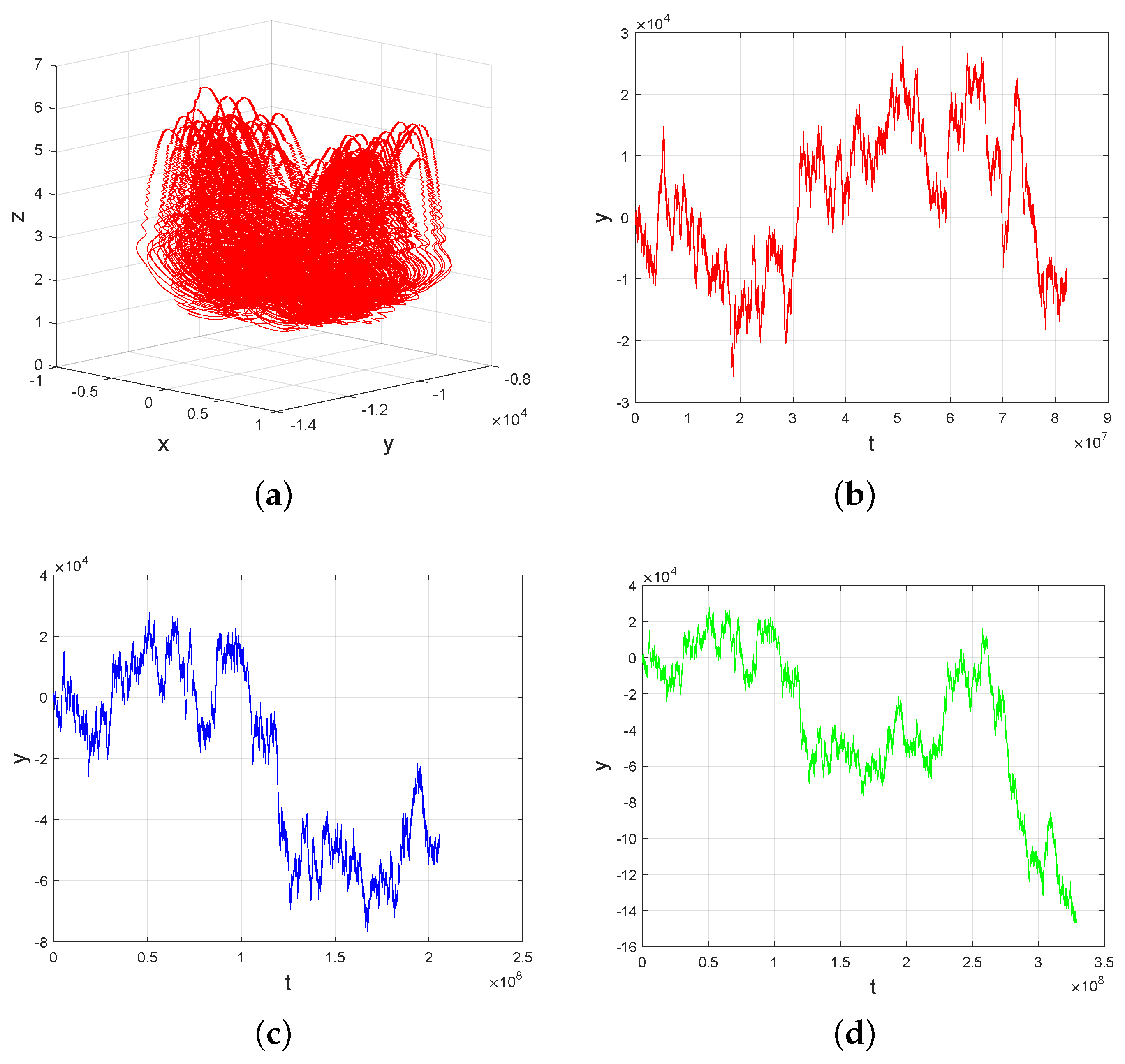
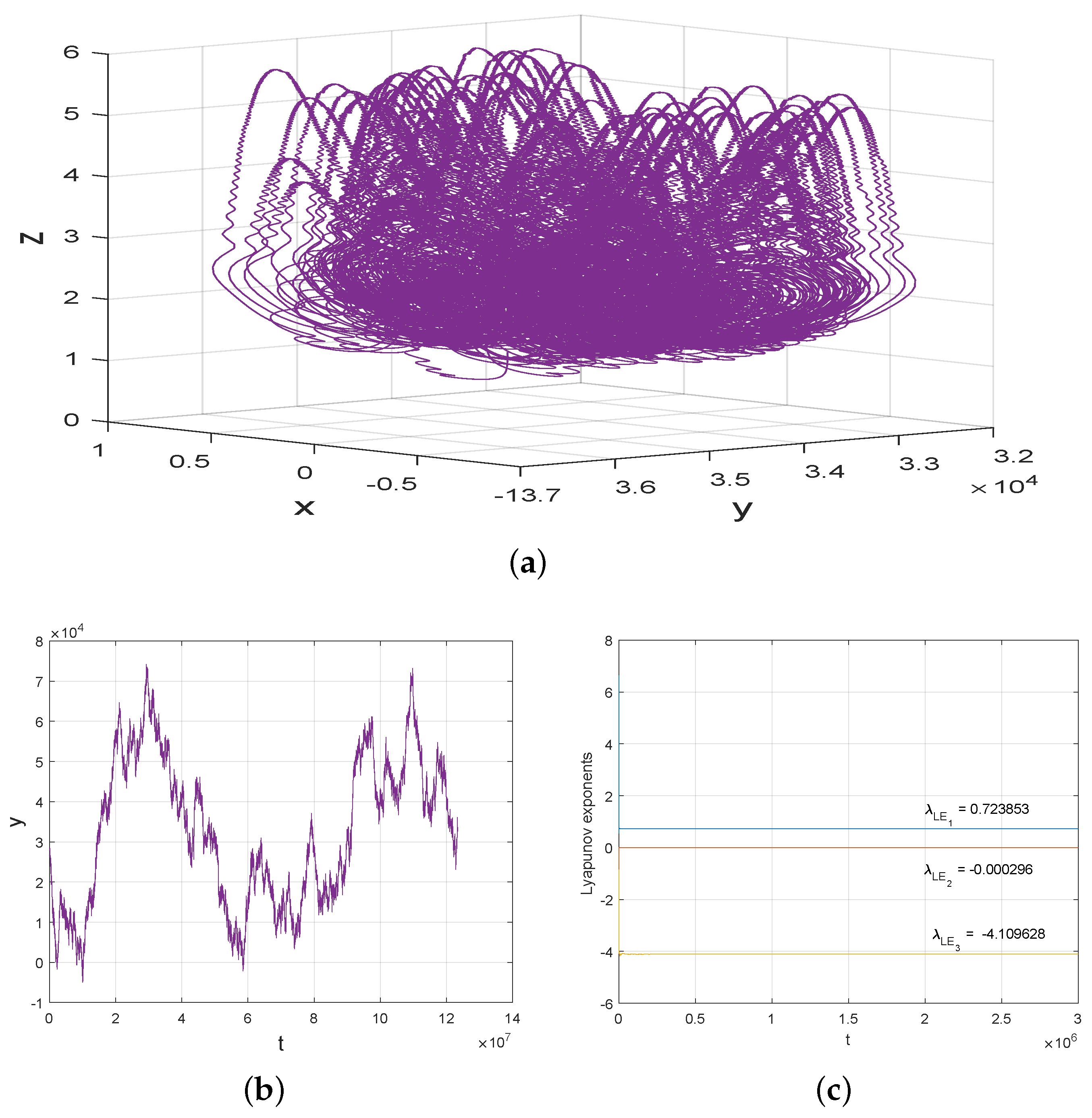
where . Particularly, when , , and , by Matlab 2016b of our computer, Figure 1, Figure 2 and Figure 3 not only illustrate the existence of the single thick two-scroll Lorenz-like attractor and stochastic behaviors of its time series of the variable y in system (1) but also that its thickness increases with time, suggesting the potential existence of unbounded two-scroll Lorenz-like attractor.
Remark 1.
Unlike those that generate infinitely many isolated identical chaotic attractors [1,2,6], Figure 2b–d exhibit the existence of a single two-scroll Lorenz-like attractor. The cause is not known, but it is thought to be the result of a combination of extreme sensitivity to the initial conditions and periodicity. Further, the stochastic feature of y may provide a reference for the study and application of finance and convection.
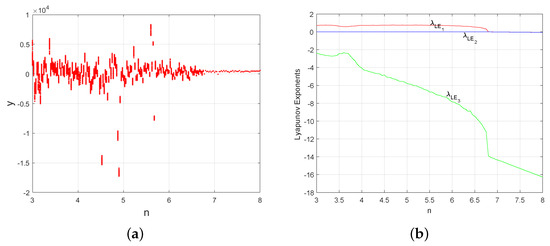
Figure 1.
When , −25, −1, and : (a) the bifurcation diagram versus ; (b) Lyapunov exponents versus .
Figure 1.
When , −25, −1, and : (a) the bifurcation diagram versus ; (b) Lyapunov exponents versus .
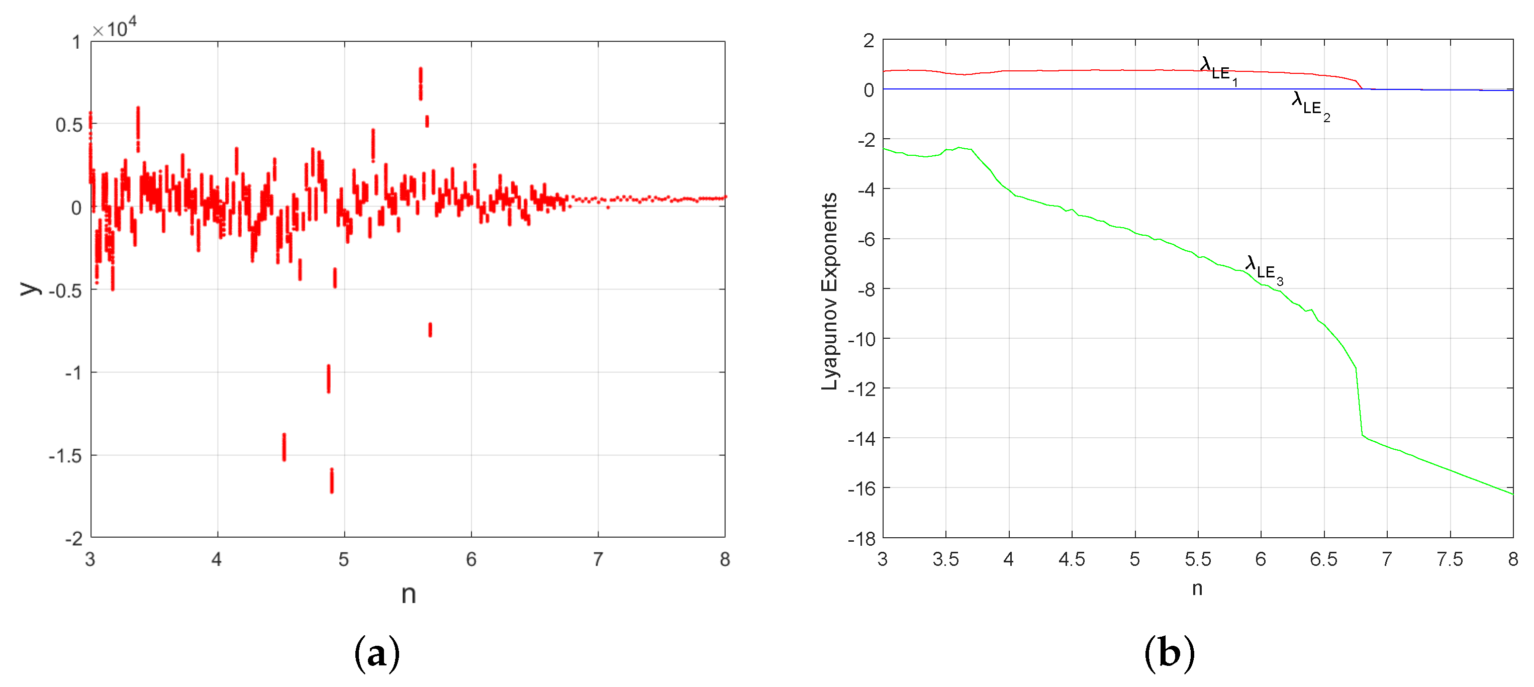

Figure 2.
When , −25, −1, and : (a,b) phase portrait and time series of the variable y of system (1) with , ; (c) time series of the variable y with , ; (d) time series of the variable y with , .
Figure 2.
When , −25, −1, and : (a,b) phase portrait and time series of the variable y of system (1) with , ; (c) time series of the variable y with , ; (d) time series of the variable y with , .
Secondly, from the algebraic structure of system (1), the distribution of equilibria is summarized in the following proposition.
Proposition 1.
(1) When , system (1) has two families of parallel lines of non-hyperbolic equilibria and .
(2) When , , and , or and , both and are two families of parallel parabolic-type non-hyperbolic equilibria.
(3) When , , and are infinitely many isolated equilibria of system (1) for , while , , and are further additional infinitely many pairs of symmetrical isolated equilibria.
To study the stability and bifurcation of equilibria, we consider the Jacobian matrix corresponding to the vector field of system (1):
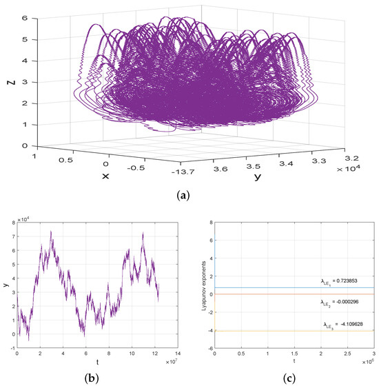
Figure 3.
(a) Thick two-scroll Lorenz-like attractor, (b) time series of the variable y, and (c) Lyapunov exponents of system (1) with , −25, −1, and , , . These figures illustrate the potential existence of unbounded two-scroll Lorenz-like attractor and stochastic behaviors of its time series of the variable y in system (1).
Firstly, the characteristic equations of points of and are
with , , and
with , .
Secondly, the characteristic equations of points of and are
with , , and
with , .
Thirdly, for and , the characteristic equations of points of and are
with , , and
with , .
While and , the ones of points of and are
with , , and
with , .
Lastly, the characteristic equations of points of and are
and
By integrating linear analysis, the Routh–Hurwitz criterion, and bifurcation theory, we have concluded the local dynamical behaviors of system (1) as follows.
Proposition 2.
(1) If , then all points of and are unstable.
(2) Set .
(2.1) If (resp. ) and (resp. ), then each of (resp. ) is stable.
(2.2) If (resp. ) and , then Hopf bifurcation occurs at each of (resp. ).
(2.3) If (resp. ) and (resp. ), then each of (resp. ) is unstable.
Proposition 3.

When , the local dynamical behaviors of each of and are totally summarized in Table 1 and Table 2. While , , (resp. , ), (resp. ), , , Table 3 and Table 4 (resp. Table 5 and Table 6) list the local dynamics of each of and . The symbols // denote the locally stable/center/unstable manifolds, as shown in [11].
Table 1.
The dynamical behaviors of points of .
Table 2.
The dynamical behaviors of points of .
Table 3.
The dynamical behaviors of points of for , .
Table 4.
The dynamical behaviors of points of for , .
Table 5.
The dynamical behaviors of points of for , .
Table 6.
The dynamical behaviors of points of for , .
Proposition 4.
Set , , , and
where
If (resp. ), then points of are asymptotically stable (resp. unstable). While , Hopf bifurcation happens at points of .
Proposition 5.
Set , , , and
where
If (resp. ), then points of are unstable (resp. asymptotically stable). If , then system (1) undergoes Hopf bifurcation at points of .
Proof outlines for Propositions 4 and 5 are detailed in Section 3.
Remark 2.
By merging numerical simulations with theoretical analysis, we illustrate singularly degenerate heteroclinic cycles with nearby chaotic attractors in the following numerical findings.
Numerical Result
Assuming . When , (resp. , ), and , the unstable manifold () (resp. ()) tends to the stable with (resp. with ), thereby forming singularly degenerate heteroclinic cycles, as shown in Figure 4a (resp. Figure 5a). Furthermore, infinitely many isolated Chen-like chaotic attractors can be generated near these heteroclinic cycles with a slight perturbation of , and Figure 4b (resp. Figure 5b) only depicts some of them.
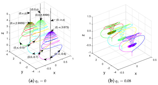
Figure 4.
Coexistence of singularly degenerate heteroclinic cycles with nearby Chen-like attractors of system (1) for , −1, −1, and , , .
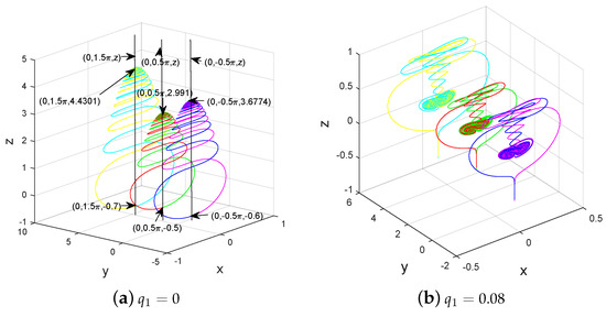
Figure 5.
Coexistence of singularly degenerate heteroclinic cycles with nearby Chen-like attractors of system (1) for , −0.1, −0.1, and , , .
For the global bifurcation on the existence of heteroclinic orbit of system (1), the following propositions summarize results, with detailed proofs provided in Section 4.
Proposition 6.
Consider , , , and . Then, the following statements are true.
Proposition 7.
Consider , , , and . Then the following assertions hold.
Proposition 8.
If , , , and , then
3. Hopf Bifurcation and Proofs of Propositions 4 and 5
The sketch of proofs of Propositions 4 and 5 is presented as follows.
Proofs of Propositions 4 and 5.
On the one hand, proofs of the stability of points of and easily follow from the Routh–Hurwitz criterion and are omitted here.
On the other hand, assume (resp. ), (resp. ), with (resp. with ).
Calculating the derivatives on both sides of Equation (2) (resp. Equation (3)) with respect to m and substituting with (resp. ) lead to
(resp.
) which validates the condition of the transversality.
Consequently, Hopf bifurcation simultaneously happens at points of (resp. ). □
By aid of the project method [11,12], we verify the nondegeneracy of the Hopf bifurcation of and by calculating Lyapunov coefficients , . Herein, we only consider the case of . The case of is similar and omitted. With the linear conversion , system (1) is changed to
i.e.,
In order to obtain , we must compute multi-linear symmetric functions below:
If , the other ones have been distilled to calculate , .
In view of the complexity of system (5), calculating the explicit form of is a challenging work now. Instead, we can manage to work out a concrete example:
Proposition 10.
If , then we obtain , , and . Therefore, the Hopf bifurcation at is supercritical, which suggests the existence of at least a stable closed orbit around each of the unstable when .
Proof.
In the light of the project method, for , we arrive at the expressions below and . Because of , the Hopf bifurcation is supercritical. In a word, set ; there is at least a stable closed orbit around each of the unstable values, i.e., , as illustrated in Figure 6. The proof is completed. □
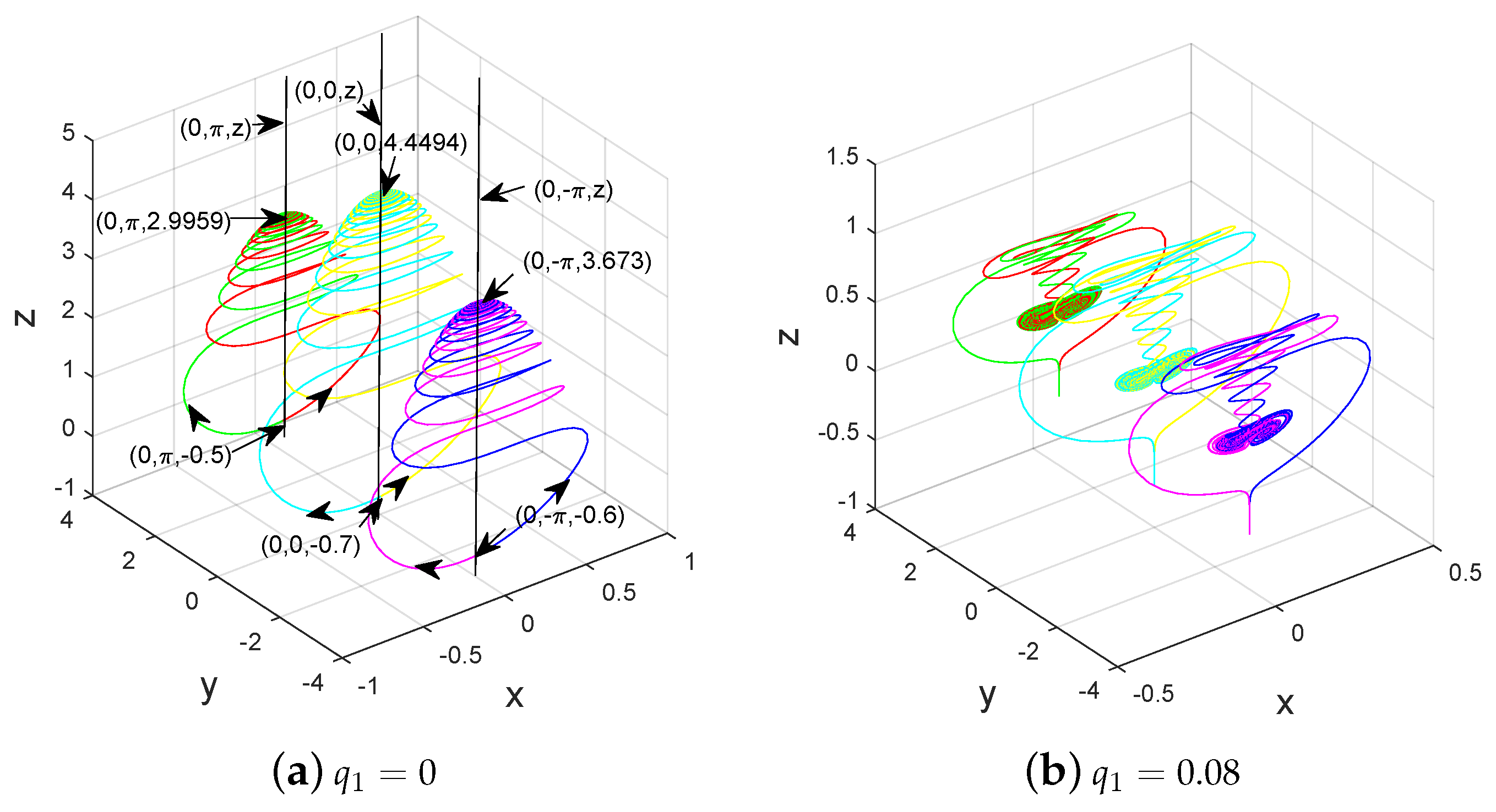
Figure 6.
Hopf bifurcation of system (1) for (a) , −0.0153, −0.1, and , , ; (b) , −1, −1, , , .
4. Existence of Heteroclinic Orbit and Proofs of Propositions 6–9
In this section, we demonstrate the existence of an infinite set of heteroclinic orbits in system (1) when (1) , , and , (2) , , , , and , (3) , and , (4) , , and .
To facilitate derivation, denote by any one solution of system (1) with the initial point . Let be the unstable manifold of system (1) at , or , or or .
Firstly, set the first Lyapunov function
the second one
the third one
and the last one
Then, the derivatives of along the trajectories of system (1) are calculated as follows:
and
respectively.
To prove Proposition 6, one introduces the following result.
Proposition 11.
When , , , and , we derive the following two assertions.
- (i)
- If ∃, such that and , then is one of the equilibrium points of system (1).
- (ii)
- If and , then , .
Proof.
(i) As in Equation (6) when , , , and , the fact , yields
In fact, implies and , , .
As a result, leads to (10).
(ii) Let us show , . Otherwise, , such that . It follows from above result (i) that is only one equilibrium point and , which contradicts the fact that . Therefore, holds for all . □
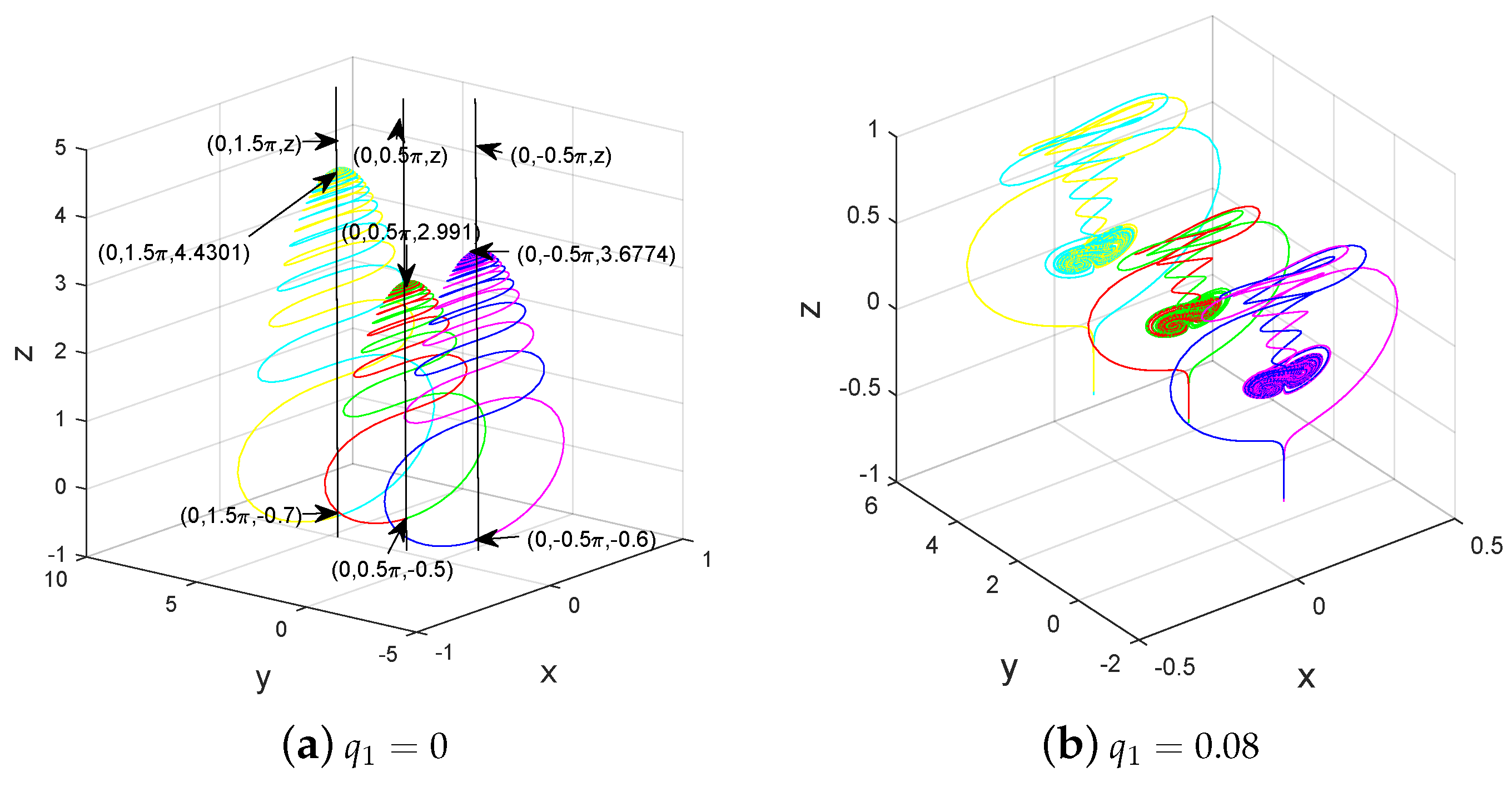
Using Proposition 11 and the method of Lyapunov function, regarding the definitions of both -limit set and -limit set [4,5,13,14,15,16,17,18,19,20,21,22], the outline of proof of Proposition 6 is sketched.
Proof of Proposition 6.
(a) Firstly, one proves that neither heteroclinic nor homoclinic orbits to or exist in system (1) when , , , and .
Suppose that (it belongs to the set of ) is a homoclinic or heteroclinic orbit to and (or and ); i.e., , where , (or , ), or (or or ). It follows from Equation (6) that
which leads to . Based on the assertion (i) of Proposition 11, is just one of the equilibria. Accordingly, there are no homoclinic/heteroclinic orbits to or in system (1).
(b) Secondly, we prove that is a heteroclinic orbit to and ; i.e., , where and . Obviously the definition of and the conclusion (ii) of Proposition 11 result in , and .
Lastly, let us show that, if there exists a heteroclinic orbit to and in system (1), then it belongs to .
Set to be any one solution of system (1) such that
where and satisfy Similar to (11), one arrives at , for all . Due to , we obtain and ; i.e.,
which leads to on the basis of assertion (ii) of Proposition 11. Since and consist of infinitely many and , there exist infinitely many heteroclinic orbits to and , which is also verified by Figure 7a. The proof is over. □
Next, to prove Proposition 7, the following statements have to be proved.
Proposition 12.
When , , , , and , we derive the following two assertions.
- (i)
- If ∃, such that and , then is one of the equilibrium points of system (1).
- (ii)
- If (or , or ), and (or , or ), then (or , or ) , .
Proof.
(i) Since when , , , and , it follows from Equation (7) that , , which thus suggests that is one of equilibria; i.e.,
Actually, implies and , , .
In a word, leads to (12).
(ii) Next, we prove that (or , or ) for all . Otherwise, suppose that (or , or ) for some . Then, the above result (i) reads that is one of equilibria of system (1) and (or , or ). This contradicts the fact that (or , or ). Hence, it follows that (or , or ) for all . □
Using Proposition 12, the outline of proof of Proposition 7 is sketched.
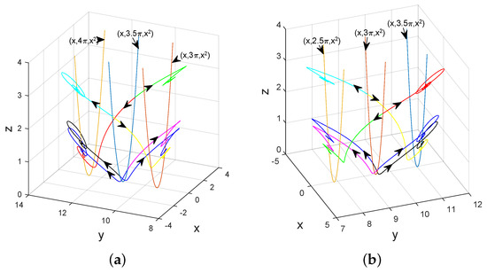
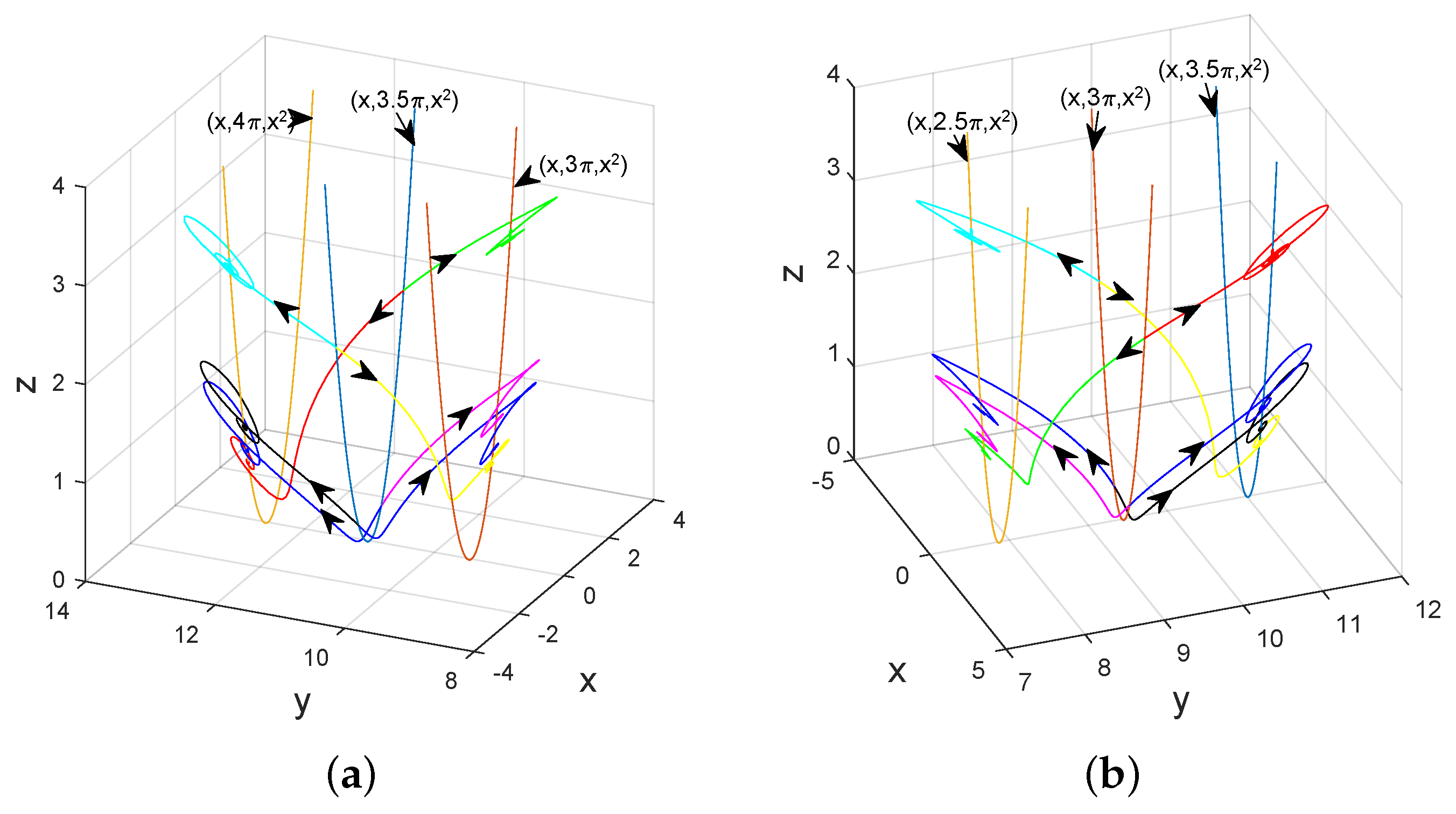
Figure 7.
Heteroclinic orbits to and , for (a) and (colored in red and green), (colored in blue and magenta), (colored in yellow and cyan), (colored in black and blue); (b) heteroclinic orbits to and , for and (colored in red and green), (colored in blue and magenta), (colored in yellow and cyan), (colored in black and blue). Both figures suggest the existence of infinitely many heteroclinic orbits to parallel parabolic-type non-hyperbolic equilibria and (or and ) when , , and (or , , and ).
Proof of Proposition 7.
(a) Let us first prove that there are no heteroclinic/homoclinic orbits to points of , , = , or in system (1) when , , , , and .
Suppose that is a homoclinic orbit of system (1) to or (or or , or or , or or ), or a heteroclinic orbit to and (or and , or and , or and ), where , (or , , or , , or , ). Namely, is a solution of system (1) such that where points and satisfy either or (or or , or ) From (7), one has
In either case, one only has the relation , which suggests . According to the assertion (i) of Proposition 12, is just one of the equilibrium points of system (1). Therefore, neither homoclinic orbits nor heteroclinic orbits to points of and (or and , or and , or and ) exist in system (1).
(b) Next, let us show that is a heteroclinic orbit to (or , or ) and ; i.e., , where (or , or ) and . From the definition of and the conclusion (ii) of Proposition 12, one can obtain (or or ) . This demonstrates that does not approach (or , or ) as . Therefore, .
Lastly, we prove that, if system (1) has a heteroclinic orbit to (or , or ) and , then this orbit belongs to .
Denote by as a solution of system (1) such that
where and satisfy or , or . Like for (13), one obtains from (7) that, for all , Since (or , or ) , we have (or , or ) and ; i.e.,
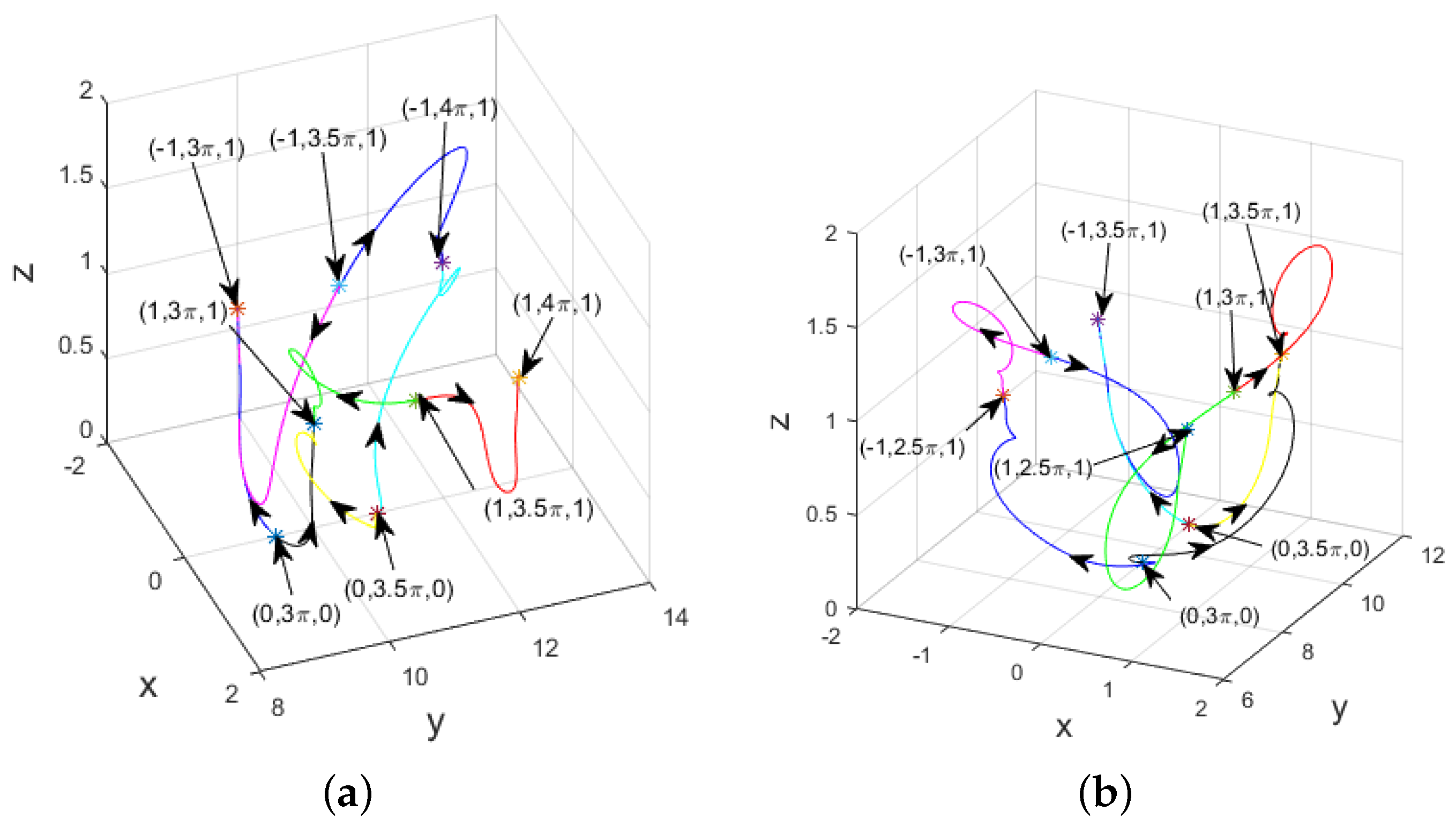
which yields based on the second assertion of Proposition 12. As , , , and contain infinitely many isolated stationary points , , or and , there exist infinitely many heteroclinic orbits to , or , or and . This theoretical result is also verified via numerical simulation, as shown in Figure 8a. The proof is over. □
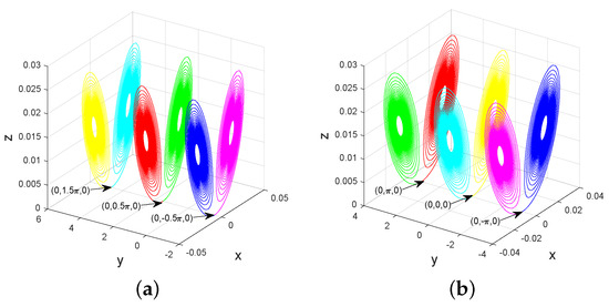
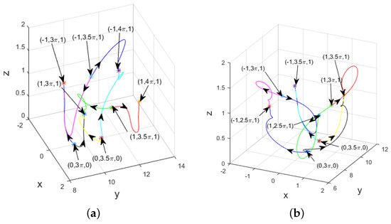
Figure 8.
(a) Heteroclinic orbits to () and , () and , , () and , , () and , for and (colored in red and green), (colored in blue and magenta), (colored in yellow and cyan), (colored in black and blue); (b) heteroclinic orbits to () and , , () and , () and , , () and , for and (colored in red and green), (colored in blue and magenta), (colored in yellow and cyan), (colored in black and blue). Both figures suggest the existence of infinitely many heteroclinic orbits to isolated stationary points of or or and (or or or and ) when , , , and (or , , , and ).
5. Conclusions
Inspired by some interesting phenomena displayed by recently reported periodically forced chaotic systems, i.e., infinitely many isolated self-excited or hidden chaotic attractors, or period cycles, or nonchaotic attractors, infinitely many scroll attractors, and even conjoined Lorenz-like attractors, etc., the authors instead tried to coin a single thick two-scroll Lorenz-like attractor that may possess the potential property of unboundedness. To reach this goal, we proposed a new simple 3D-extended Lorenz-like system with two sine functions, which not only generates the desirable attractor but also has three types of heteroclinic orbits to two families of parallel parabolic-type non-hyperbolic equilibria, two families of infinitely many pairs of isolated equilibria, an infinite set of isolated equilibria, and infinitely many pairs of isolated equilibria.
Since Figure 2b,d illustrate some certain stochastic characteristics in the time series of state variable y of that thick two-scroll Lorenz-like attractor, one should manage to determine the boundedness of it in the follow-up study of this research when because the size of a thick two-scroll Lorenz-like attractor depends on that of y. In addition, one needs to undertake research and analysis on singularly degenerate heteroclinic cycles, hidden attractors, homoclinic orbits, and so on.
Author Contributions
Conceptualization, J.P. and H.W.; Methodology, H.W.; Software, J.P. and G.K.; Validation, H.W. and G.K.; Visualization, G.K. and F.H.; Writing—original draft, J.P.; Writing—review and editing, H.W. All authors have read and agreed to the published version of the manuscript.
Funding
This work is supported in part by National Natural Science Foundation of China under Grant 12001489, in part by Zhejiang Public Welfare Technology Application Research Project of China under Grant LGN21F020003, in part by Natural Science Foundation of Taizhou University under Grant T20210906033, and in part by Natural Science Foundation of Zhejiang Guangsha Vocational and Technical University of Construction under Grant 2022KYQD-KGY.
Data Availability Statement
Data are contained within the article.
Conflicts of Interest
The authors declare no conflict of interest.
References
- Zhang, X.; Chen, G. Constructing an autonomous system with infinitely many chaotic attractors. Chaos Interdiscip. J. Nonlinear Sci. 2017, 27, 071101. [Google Scholar]
- Yang, T.; Yang, Q. A 3D autonomous system with infinitely many chaotic attractors. Int. J. Bifurc. Chaos 2019, 29, 1950166. [Google Scholar]
- Zhang, X. Boundedness of a class of complex Lorenz systems. Int. J. Bifurc. Chaos 2021, 31, 2150101. [Google Scholar] [CrossRef]
- Wang, H.; Ke, G.; Pan, J.; Su, Q. Conjoined Lorenz-Like Attractors Coined. Miskolc Mathematical Notes, Code: MMN-4489. 2023. Available online: http://mat76.mat.uni-miskolc.hu/mnotes/forthcoming?volume=0&number=0 (accessed on 19 March 2025).
- Wang, H.; Pan, J.; Ke, G. Revealing more hidden attractors from a new sub-quadratic Lorenz-like system of degree 65. Int. J. Bifurc. Chaos 2024, 34, 2450071. [Google Scholar] [CrossRef]
- Kuate, P.; Fotsin, H. Complex dynamics induced by a sine nonlinearity in a five-term chaotic system FPGA hardware design and synchronization. Chaos 2020, 30, 123107. [Google Scholar] [PubMed]
- Sahoo, S.; Roy, B.K. Design of multi-wing chaotic systems with higher largest Lyapunov exponent. Chaos Solitons Fractals 2022, 157, 111926. [Google Scholar]
- Olkhov, V. Expectations, price fluctuations and Lorenz attractor. MPRA Pap. 2018, 1–29. Available online: https://mpra.ub.uni-muenchen.de/89222/ (accessed on 19 March 2025).
- Zhang, X.; Chen, G. Impulsive systems with growing numbers of chaotic attractors. Chaos Interdiscip. J. Nonlinear Sci. 2022, 32, 071102. [Google Scholar] [CrossRef] [PubMed]
- Zhou, Z.; Tigan, G.; Yu, Z. Hopf bifurcations in an extended Lorenz system. Adv. Diff. Eqs. 2017, 28, 1–10. [Google Scholar] [CrossRef]
- Kuzenetsov, Y.A. Elements of Applied Bifurcation Theory, 3rd ed.; Springer: New York, NY, USA, 2004; Volume 112. [Google Scholar]
- Sotomayor, J.; Mello, L.F.; Braga, D.C. Lyapunov coefficients for degenerate Hopf bifurcations. arXiv 2007, arXiv:0709.3949. [Google Scholar]
- Wang, H.; Pan, J.; Hu, F.; Ke, G. Asymmetric singularly degenerate heteroclinic cycles. Int. J. Bifurc. Chaos 2025, 2550072. [Google Scholar] [CrossRef]
- Pan, J.; Wang, H.; Hu, F. Revealing asymmetric homoclinic and heteroclinic orbits. Electron. Res. Arch. 2025, 33, 1337–1350. [Google Scholar]
- Li, T.; Chen, G.; Chen, G. On homoclinic and heteroclinic orbits of the Chen’s system. Int. J. Bifurc. Chaos 2006, 16, 3035–3041. [Google Scholar] [CrossRef]
- Tigan, G.; Llibre, J. Heteroclinic, homoclinic and closed orbits in the Chen system. Int. J. Bifurc. Chaos 2016, 26, 1650072. [Google Scholar] [CrossRef]
- Chen, Y.; Yang, Q. Dynamics of a hyperchaotic Lorenz-type system. Nonlinear Dyn. 2014, 77, 569–581. [Google Scholar] [CrossRef]
- Tigan, G.; Constantinescu, D. Heteroclinic orbits in the T and the Lü system. Chaos Solitons Fractals 2009, 42, 20–23. [Google Scholar] [CrossRef]
- Liu, Y.; Yang, Q. Dynamics of a new Lorenz-like chaotic system. Nonl. Anal. RWA 2010, 11, 2563–2572. [Google Scholar]
- Liu, Y.; Pang, W. Dynamics of the general Lorenz family. Nonlinear Dyn. 2012, 67, 1595–1611. [Google Scholar] [CrossRef]
- Li, X.; Ou, Q. Dynamical properties and simulation of a new Lorenz-like chaotic system. Nonlinear Dyn. 2011, 65, 255–270. [Google Scholar] [CrossRef]
- Li, X.; Wang, P. Hopf bifurcation and heteroclinic orbit in a 3D autonomous chaotic system. Nonlinear Dyn. 2013, 73, 621–632. [Google Scholar]

Disclaimer/Publisher’s Note: The statements, opinions and data contained in all publications are solely those of the individual author(s) and contributor(s) and not of MDPI and/or the editor(s). MDPI and/or the editor(s) disclaim responsibility for any injury to people or property resulting from any ideas, methods, instructions or products referred to in the content. |
© 2025 by the authors. Licensee MDPI, Basel, Switzerland. This article is an open access article distributed under the terms and conditions of the Creative Commons Attribution (CC BY) license (https://creativecommons.org/licenses/by/4.0/).