Abstract
When extreme values or outliers occur in asymmetric datasets, conventional mean estimation methods suffer from low accuracy and reliability. This study introduces a novel class of robust Särndal-type mean estimators utilizing re-descending M-estimator coefficients. These estimators effectively combine the benefits of robust regression techniques and the integration of extreme values to improve mean estimation accuracy under simple random sampling. The proposed methodology leverages distinct re-descending coefficients from prior studies. Performance evaluation is conducted using three real-world datasets and three synthetically generated datasets containing outliers, with results indicating superior performance of the proposed estimators in terms of mean squared error (MSE) and percentage relative efficiency (PRE). Hence, the robustness, adaptability, and practical importance of these estimators are illustrated by these findings for survey sampling and more generally for data-intensive contexts.
Keywords:
robust re-descending estimators; Särndal-type mean estimators; outliers; survey sampling; mean squared error MSC:
62D05
1. Introduction
In each stage of the normal research process, the first step is the administration of a sample survey because it is one of the basic approaches for data collection. Interviews can be conducted in various ways: virtually, at the person or group level, or through mail, online, or in person. Questionnaires are a common research method adopted in many disciplines, including education, health, income and expenditure, employment, industry, business, animals, and the environment. The techniques permitted for conducting surveys are face-to-face, telephone, mail, and interviews. Surveys can only go wrong if the methodology used to gather the data is flawed, as the data are crucial for reaching the correct conclusion. Thus, it is possible to use an action-plan based on proper strategies focused on implementation, which may enhance the methods that promote the quality of research and lead to higher accuracy of results. One of these methods is the utilization of technical auxiliary variables, which are data points most closely associated with the primary variable of study. The inclusion of such associated variables makes it better than the model being used, hence providing effective and reliable solutions most of the time (Bhushan and Kumar [1]).
In many populations, the presence of extreme values can significantly impact the estimation of unknown population characteristics. Failure to observe these values leads to certain estimates that are very sensitive and can be either overestimated or underestimated in some instances. As a result, the accuracy of traditional estimators, measured by MSE, tends to decline when extreme values are present in the dataset. Despite the fact that such data points might sometimes be omitted from analysis, their collection is essential to enhance the reliability of the population estimates. For instance, Mohanty and Sahoo [2] proposed two linear transformations of the smallest and largest observations of an auxiliary variable to develop more robust estimators. However, further exploration of these methods was limited until Khan and Shabbir [3] extended the use of extreme values to various finite population mean estimators. Furthermore, Daraz et al. [4] used a sampling method known as stratified random sampling to improve the estimation of finite population means in cases where outliers are prevalent. For further discussion and developments in this area, consult [5,6,7] and related works.
We often see a widespread use of the arithmetic mean as a measure of central tendency. It is also a very useful method of measuring location and has been successfully used in a wide spectrum of sciences and arts. Consequently, improving mean estimation methods is essential not only in survey sampling but also in numerous other fields. Accurate mean estimation becomes particularly critical in the presence of extreme observations, a common challenge in sampling surveys (Koc and Koc [8]). To address this issue, efficient methods based on ratio and regression for mean estimation are utilized. Additionally, several techniques that consider extreme values of the augmented dataset are employed. For example, Mohanty and Sahoo [2] initially used linear transformations to determine the lower and upper limits of the auxiliary variable. These transformations demonstrated the efficiency of ratio estimators, even when traditional ratio estimators performed worse than the simple mean per unit estimator. Khan and Shabbir [3] introduced modified ratio, product, and regression-type estimators using minimum and maximum values, with numerical evidence confirming improved efficiency. Khan and Shabbir [3] further expanded this work under double sampling in Khan [9]. Similarly, Cekim and Cingi [5] developed ratio, product, and exponential-type estimators of the population mean by applying novel linear transformations based on known minimum and maximum values of auxiliary variables. Shahzad et al. [6] advanced this concept by designing separate mean estimators under stratified random sampling, incorporating quantile regression and extreme values using the Särndal approach. They also extended their methods to sensitive topics using scrambled response models. More recently, Anas et al. [7] adapted the work of Shahzad et al. [6] and introduced robust mean estimators for simple random sampling. These developments show that it is possible to increase the accuracy of mean estimation by using extremes while varying different sampling situations.
Previous studies have incorporated either ratio and product techniques or regression models, using ordinary as well as robust coefficients to account for outliers. However, no existing mean estimator integrates re-descending M-estimators with extreme values simultaneously. The Särndal technique appears to present a promising avenue for integrating re-descending M-estimators with extreme/contaminated values to improve the estimation of the mean. This notable gap in the literature has inspired us to propose a new class of Särndal-type mean estimators that leverage re-descending coefficients.
The remaining article is structured into multiple sections. In Section 2, re-descending mean estimators are defined as a robust alternative to the ordinary least squares (OLS) method for treating asymmetric data with outliers. The concept is extended in Section 3 by adapting Särndal’s [10] mean estimator to improve efficiency in the presence of extreme values. A new family of re-descending regression-based mean estimators is proposed, incorporating re-descending coefficients developed by various researchers. Section 4 evaluates the proposed methodology using real-world and synthetic datasets, demonstrating lower MSE and higher PRE compared to adapted methods. The article concludes in Section 5.
2. Re-Descending M-Estimators and Mean Estimation
In many real-life situations, the OLS method is used. However, when applying the assumption of the simple normality of the error terms in OLS regression, we encounter problems in real-life data, especially due to outliers. Any type of outlier can significantly impact the OLS estimate, rendering the result inefficient and inaccurate even with the addition of another observation to the model (Dunder et al. [11]). In an attempt to address this problem, scientists have created a stable method of regression analysis known as robust regression that carries out modifications on OLS. This is particularly relevant in large sample settings with asymmetric distribution, as OLS estimates are sensitive to outliers, and the solution lies in robust M-estimators.
Based on work concerning the characterization of the sensitivity of linear regression methods to outliers, Huber [12] developed the M-estimator. This estimator assigns a value close to 1 for the middle value and nearly zero for the most extreme values. In conditions where the OLS assumption of normally distributed error terms does not hold, the M-estimator also works within the maximum likelihood estimation framework. The robust M-estimators replace the squared error term in OLS by a symmetric loss function, defined as follows:
The previous literature shows that the M-estimator achieves its minimum value using IRLS optimization iterations. The loss function distributes outlier weights to improve performance efficiency.
Then, the associated influence function, , is obtained by differentiating the loss function with respect to the residuals
where are the covariates. The weight function is
Re-descending M-estimators are derived by modifying the loss function to exhibit a re-descending nature. This concept has been well explored in the literature by Beaton and Tukey [13], Qadir [14], Alamgir et al. [15], Khalil et al. [16], Noor-ul-Amin et al. [17], Anekwe and Onyeagu [18], and Luo et al. [19]. In fact, these estimators are very powerful in eliminating the influence of outliers on the subsequent statistical results.
The mean, as discussed in earlier sections, is a basic way to summarize central tendency. In this study, we utilize re-descending M-estimator regression coefficients to estimate the mean efficiently. Specifically, re-descending M-estimators developed by Noor-ul-Amin et al. [17], Khan et al. [20], Anekwe and Onyeagu [18], and Raza et al. [21,22] will be employed for this purpose.
2.1. Existing Re-Descending Estimators
In order to handle data contaminated with outliers, Noor-ul-Amin et al. [17] proposed a re-descending estimator. Their methodology minimizes the influence of large residuals by applying a weight function. The estimator is adjustable, so that tuning parameters c and a determine its robustness and efficiency, making it suitable for robust regression. The primary contribution of Noor-ul-Amin et al. [17] was to demonstrate that their estimator performs well across a variety of contamination scenarios. Their objective , Psi , and weight functions are given below.
Objective function:
Psi function:
Weight function:
where is the residual and is the tuning constant.
In Khan et al. [20], a new re-descending M-estimator based on the hyperbolic tangent function is introduced. Their proposed objective function needs to be smooth and continuous to achieve high efficiency and robustness. This estimator also performs well on asymmetric heavy-tailed data distributions. A hyperbolic cosine-based weight function is used to make the method insensitive to noise and give full weight to central observations in the regression model. The objective, Psi, and weight functions are provided below.
Objective function:
Psi function:
Weight function:
Anekwe and Onyeagu [18] developed a re-descending estimator with a focus on polynomial-based weight functions. For residuals above the threshold of c, their weight function transitions smoothly to zero. It provides a high breakdown point and should be robust against leverage points. The objective, Psi, and weight functions are provided below.
Objective function:
Psi function:
Weight function:
Raza et al. [21] introduced an estimator that is based on parameterized robustness principles. Similar to Noor-ul-Amin et al. [17], their weight function balances efficiency and robustness parameters k and a. The objective, Psi, and weight functions are detailed below.
Objective function:
Psi function:
Weight function:
where k and a are arbitrary and generalized tuning constants, respectively.
Raza et al. [22] introduced a higher-order polynomial re-descending estimator, characterized by its ability to reject extreme outliers while maintaining efficiency in central data regions. The objective, Psi, and weight functions are detailed below.
Objective function:
Psi function:
Weight function:
where a is the tuning constant.
2.2. Adaptive Mean Estimators Using Re-Descending Coefficients
Ratio estimation is a valuable method for estimating the population mean when there is a positive linear relationship between the supplementary and study variables in survey sampling. This approach was pioneered in the mid-twentieth century by Cochran and has become a major methodological achievement that is widely used not only in the study of agriculture but also in many other research fields. We refer readers to Cochran [23], Cetin and Koyuncu [24], and Daraz et al. [25] for more information about ratio-type estimators. Pioneers of ratio-type estimators based on OLS regression coefficients are Kadilar and Cingi [26]. In the presence of outliers, traditional OLS regression is not adequate or satisfactory. This limitation is overcome in Kadilar et al. [27], who suggested using robust regression methods with the ratio-type estimator to improve the precision and reliability of the ratio-type estimator. They utilized Huber-M regression, a robust regression method, for ratio type mean estimation in a simple random sampling scheme. Building on these foundational studies, we introduce a modified family of estimators under simple random sampling with re-descending coefficients using approaches from Noor-ul-Amin et al. [17], Khan et al. [20], Anekwe and Onyeagu [18], and Raza et al. [21,22]
The adapted family contains , and . The characteristics of study variable Y and the auxiliary variable X are denoted as sample means, and , respectively, and the population mean of the auxiliary variable X is . The MSE of the adapted class is as follows:
The MSE of the adapted family contains a finite population correction factor , the ratio of means of study and auxiliary variables , the variance of study and auxiliary variables , , and re-descending coefficients .
3. Proposed Family of Re-Descending Estimators
Being an outlier does not mean it is an anomaly; it could actually be an important source of information about the structure or variation in a dataset (Zaman et al. [28]). Traditional analysis methods do not typically capture the population-specific characteristics or trends that can be inferred from outliers. Särndal [10] recognized this potential, and introduced a mean estimator with the purpose of accounting for the impact of extreme values while keeping asymptotic efficiency. In contrast to conventional mean estimation approaches, this method adjusts for the presence of extreme values automatically. The Särndal [10] mean estimator is defined as follows:
where is a wisely chosen constant. Let N be the size of population and n be the size of sample. The minimum variance of is given below by using
In light of Särndal [10], and extending the idea of Mukhtar et al. [29], we propose a family of re-descending regression-based mean estimators for the estimation of . Normally, when the degree of linear relationship between the research variable Y and the auxiliary variable X greater than 0, the choice of is to be expected, and the . Utilizing this type of setup under simple random sampling, we define the new family of re-descending regression coefficient-based estimators as follows:
where can be any of the re-descending coefficients , , , , in this case. In addition, , , and are the chosen constants. For the results related to theoretical MSE, let us explain the notations as follows:
By expanding
The MSE of is obtained by squaring both sides of Equation (8) and ignoring terms with s that have powers larger than two
Note that every notation utilized in has been effectively depicted in the preceding lines. Furthermore, our newly built class can be organized in the structure of Särndal [10]. However, we are implementing their framework using re-descending regression-type mean estimators. By leveraging known outcomes and performing simple mathematical calculations, we avoid tedious or unnecessary computations to provide the optimal values of and, consequently, the minimum MSE final expressions of the estimators as follows:
It is important to note that we are using five re-descending coefficients in our estimation process. The calculation of these coefficients for the five re-descending estimators involves an iterative process aimed at achieving robust estimation by minimizing the influence of outliers. Each estimator applies a unique weight function, , designed to diminish the impact of large residuals in alignment with its defined structure. As a baseline, the OLS method is used for the first estimate of (say). Following this, a weighted least squares procedure is performed iteratively, with residual weights updated at each iteration t, such that . Convergence is reached when , until the process reaches an iteration where is defined as the tolerance level. To make the article more comprehensive for the readers, we replace with , , , , and consider five individuals of the proposed class with their minimum-MSE as given below:
4. Numerical Study
In this section, we assess the performance of the proposed and adapted estimators by applying them to three real-world datasets and three synthetically generated datasets.
4.1. Real Life Applications
Populations 1 and 2:
The education expenditure dataset from the R robustbase package is utilized as Population-1. This dataset includes variables related to education expenditure across the 50 U.S. states. X represents the number of residents per thousand in urban areas in 1970, and Y represents per capita expenditure on public education in 1975, all concurrently. For Population-2, the same dataset is employed, where the dependent variable Y remains unchanged from Population-1, and the auxiliary variable X is replaced with the per capita personal income from 1973.
Population-3:
Farm loans data provided by Singh [30] are used as Population-3. In this dataset, Y measures the value of real estate loans issued, and X measures the value of non -real estate farm loans issued, in 1977.
The relevant characteristics of these populations are detailed in Table 1. Figure 1, Figure 2 and Figure 3 corresponding to populations [1, 2, 3] reveal an asymmetric distribution and the presence of outliers, making them well-suited for evaluating the performance of the proposed estimators. The MSE results for these real-world populations are presented in Table 2.

Table 1.
Characteristics of real populations.
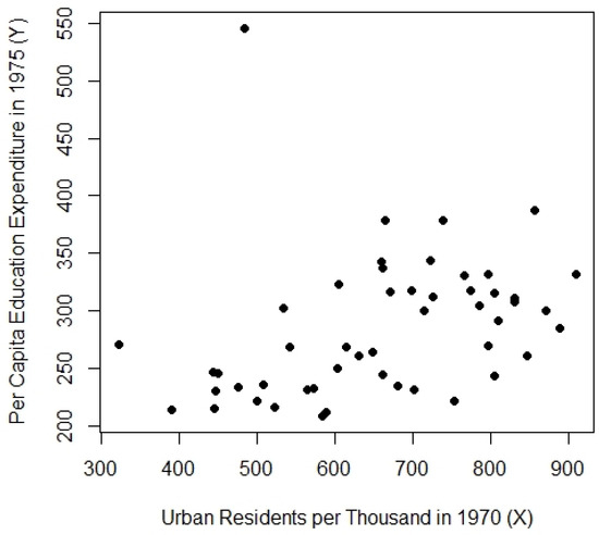
Figure 1.
Scatter plot for Population-1.
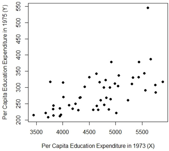
Figure 2.
Scatter plot for Population-2.
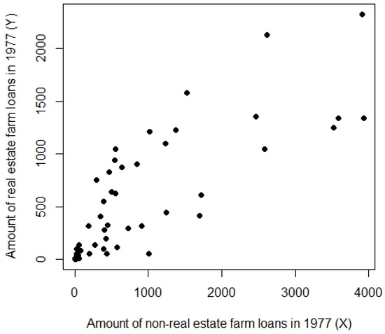
Figure 3.
Scatter plot for Population-3.
Table 2.
MSE using Populations 1, 2, 3.
4.2. Data Generations and Simulation Study
In this article, a simulation study was conducted to evaluate the performance of the proposed re-descending estimators under various artificially generated populations, including the presence of outliers. The details of these populations will be provided in the following lines.
Populations 4, 5, and 6:
The independent variable X for Populations 4, 5, and 6 was generated from the following distributions:
uniform distribution ;
gumbel distribution ;
weibull distribution .
The dependent variable Y was generated following a linear relationship described as follows:
where . In order to create outliers for a given Y, the data was perturbed by adding large deviations drawn from another normal distribution , as outliers are extremely different from the other data of Y. Five random indices were chosen, and the corresponding Y was perturbed with large deviations from another normal distribution N. This approach generated real datasets containing a blend of regular observations and outliers, matching real cases in which outliers may occur due to measurement errors or extreme events. The generated datasets comprised 100 observations, with both the regular data points and the outliers visualized in a scatterplot for clarity, see Figure 4, Figure 5 and Figure 6. The behavior of the outliers was clearly differentiated from standard points by showing the results in red. These artificial datasets were generated for simulation studies and provide a robust framework for testing the effectiveness of re-descending M-estimators in identifying and mitigating the influence of outliers on regression based mean estimation. The simulated MSE results of these artificial populations are provided in Table 3.
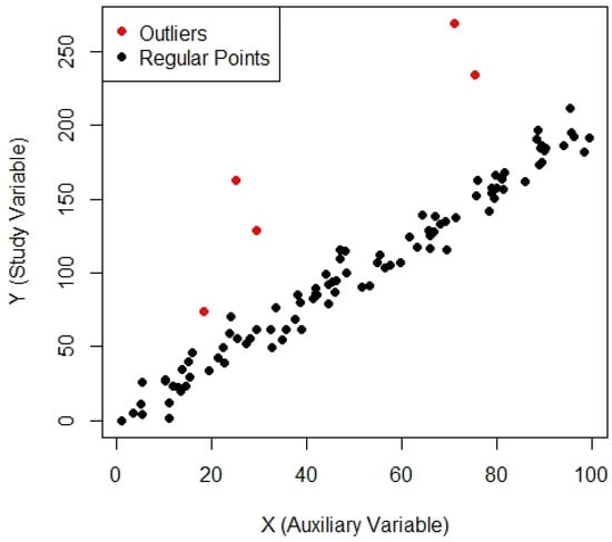
Figure 4.
Scatter plot for Population-4.
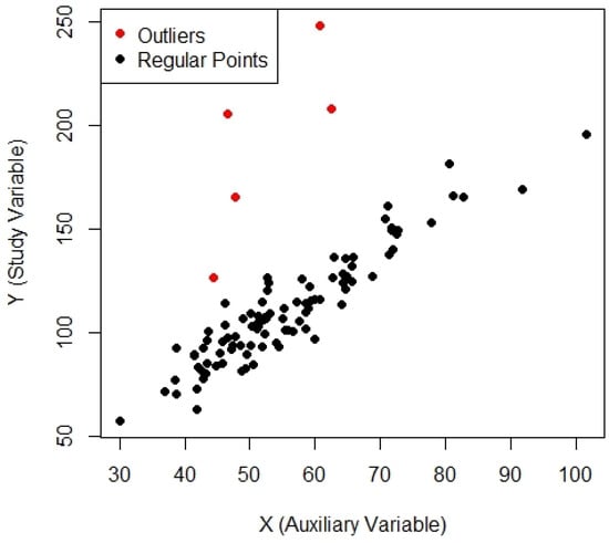
Figure 5.
Scatter plot for Population-5.
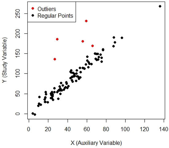
Figure 6.
Scatter plot for Population-6.
Table 3.
MSE using Populations 4, 5, 6.
The comparison plot for Populations 1–6 are illustrated in Figure 7, Figure 8, Figure 9, Figure 10, Figure 11 and Figure 12.
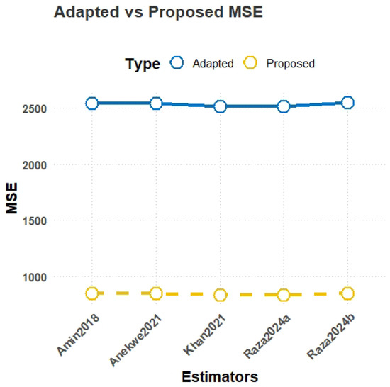
Figure 7.
MSE comparison plot for Population-1.
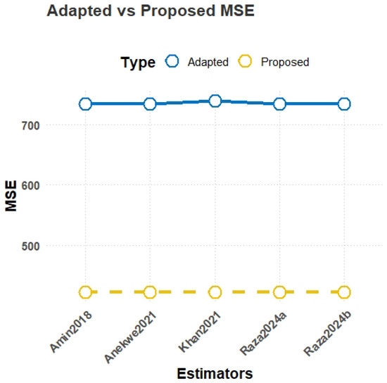
Figure 8.
MSE comparison plot for Population-2.
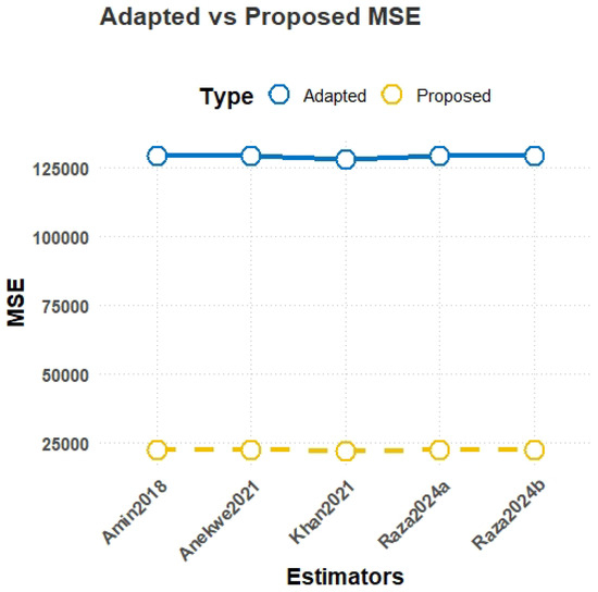
Figure 9.
MSE comparison plot for Population-3.
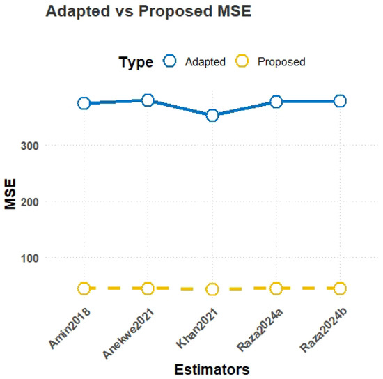
Figure 10.
MSE comparison plot for Population-4.
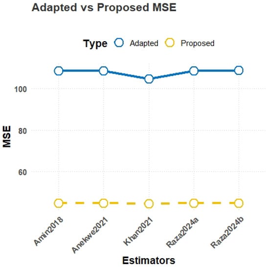
Figure 11.
MSE comparison plot for Population-5.
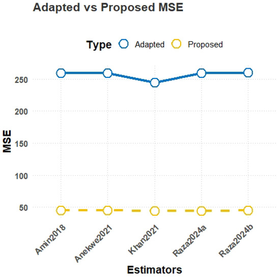
Figure 12.
MSE comparison plot for Population-6.
4.3. Interpretation of Results
- MSE results from Table 2:The results in Table 2 demonstrate the consistent superiority of the proposed estimators () over the existing estimators () across all three populations. For Population-1, representing education expenditure data, the lowest MSE is achieved by the proposed estimator with a value of 837.93, significantly outperforming the best-performing existing estimator, , which has an MSE of 2515.49. Similarly, in Population-2, another case of education expenditure data, again achieves the lowest MSE of 423.39, while the highest-performing existing estimator, , records an MSE of 733.88. For Population-3, based on farm loans data, the trend persists, with yielding the lowest MSE of 22,185.60, compared to the much higher value of 129,184.3 observed for .
- MSE results from Table 3:For Population-4, which is uniformly distributed, the proposed estimator achieves the lowest MSE of 44.58, significantly outperforming the best-performing existing estimator with an MSE of 352.73, demonstrating the superior efficiency of the proposed class for uniformly distributed data. In Population-5, generated from a Gumbel distribution, emerges as the most robust with an MSE of 44.67, which is considerably better than the existing estimator with an MSE of 108.66, indicating strong performance in handling skewed data with heavy tails. Similarly, for Population-6, simulated from a Weibull distribution, the proposed estimator achieves the lowest MSE of 44.70 compared to the best-performing existing estimator , which has an MSE of 259.03. These simulations demonstrate the robustness, adaptability, and efficiency of the proposed estimators for asymmetric data.
-
Table 4. PRE using Population-1.
Table 5. PRE using Population-2.
Table 6. PRE using Population-3.
Table 7. PRE using Population-4.
Table 8. PRE using Population-5.
Table 9. PRE using Population-6.The results from Table 4, Table 5, Table 6, Table 7, Table 8 and Table 9 illustrate the superior performance of the proposed estimators in terms of percentage relative efficiency (PRE) across all populations. For Population-1, Table 4 shows that the proposed estimator achieves the highest PRE of 304.03, reflecting substantial efficiency gains over existing methods. Similarly, for Population-2, as presented in Table 5, stands out with a PRE of 174.47, outperforming all other estimators. Table 6 in Population-3 displays that has the highest PRE of 579.38 and, thus, has a very good performance in coping with data outliers. For simulated datasets, Table 7 shows that achieves a significant PRE improvement of 785.99 in Population-4, emphasizing its efficiency in uniformly distributed data. Similarly, for Population-5, Table 8 demonstrates that maintains the highest PRE at 234.42, far surpassing the performance of existing methods. Finally, Table 9 shows that once again, emerges with a PRE of 547.58 for Population-6, making it the most adaptable and robust estimator tested on different datasets. Overall, the proposed estimators consistently outperform existing methods in all scenarios, making them highly effective and efficient in robust re-descending regression-based mean estimation.
- Summary of ResultsAll evaluated populations and scenarios are well served by the proposed re-descending regression-based estimators, which consistently show superior performance. Both of the proposed estimators demonstrate robustness and adaptability in terms of MSE and PRE compared with adapted methods. Especially in cases where datasets contain outliers or asymmetric data, conventional estimators are unable to maintain efficiency. The findings confirm the effectiveness of the proposed methodology and its great potential for application in real-world data analysis and survey sampling.
4.4. Limitations of the Study
It is shown that the proposed re-descending Särndal-type mean estimators offer significant improvements in robustness and accuracy but some limitations should be noted. The study also begins with SRS as the main focus of study, while the performance of the proposed estimators under more complex sampling schemes, such as stratified, cluster, and systematic sampling, is still an area for further research. Secondly, these estimators are particularly fruitful when extreme values are present in the dataset.
5. Conclusions
This study presents a novel class of robust Särndal-type mean estimators utilizing re-descending M-estimator coefficients to effectively address the challenges posed by outliers and extreme values in diverse datasets. By incorporating advancements from prior works, such as those by Noor-ul-Amin et al. [17], Khan et al. [20], Anekwe and Onyeagu [18], and Raza et al. [21,22], the proposed estimators significantly improve the accuracy and efficiency of mean estimation, as evidenced by lower MSE and higher PRE compared to adapted methods. These estimators demonstrate remarkable robustness and adaptability across real-world datasets, such as education expenditure and farm loans, as well as simulated datasets derived from uniform, Gumbel, and Weibull distributions. Their practical utility in survey sampling and related fields is due to their ability to maintain reliability and accuracy in the presence of asymmetry and outliers. In addition, these results suggest that these estimators might be applicable for applications in which robust data analysis is important, including economics, health, and the social sciences. Future work could be aimed at extending these methodologies to more complicated sampling frameworks such as [31] and using them in interdisciplinary settings more generally.
Author Contributions
Conceptualization, U.S.; formal analysis, U.S. and I.A.; funding acquisition, K.A.R. and A.T.A.; methodology, T.S.A., K.M.K.A., U.S., T.M. and I.A.; project administration, A.T.A.; software, K.A.R. and U.S.; supervision, J.S.; writing—original draft, K.A.R., A.T.A., T.S.A., K.M.K.A., U.S., J.S., T.M. and I.A.; writing—review and editing, K.A.R., A.T.A., T.S.A., K.M.K.A., U.S., J.S. and T.M. All authors have read and agreed to the published version of the manuscript.
Funding
This research has been funded by the Scientific Research Deanship at the University of Ha’il- Saudi Arabia through project number RG-24 067.
Data Availability Statement
All the relevant data are available within the manuscript.
Conflicts of Interest
The authors declare no conflicts of interest.
References
- Bhushan, S.; Kumar, A. Optimal classes of estimators for population mean using higher order moments. Afr. Mat. 2025, 36, 12. [Google Scholar]
- Mohanty, S.; Sahoo, J. A note on improving the ratio method of estimation through linear transformation using certain known population parameters. Sankhyā Indian J. Stat. Ser. B 1995, 57, 93–102. [Google Scholar]
- Khan, M.; Shabbir, J. Some improved ratio, product, and regression estimators of finite population mean when using minimum and maximum values. Sci. World J. 2013, 2013, 431868. [Google Scholar]
- Daraz, U.; Shabbir, J.; Khan, H. Estimation of finite population mean by using minimum and maximum values in stratified random sampling. J. Mod. Appl. Stat. Methods 2018, 17, 20. [Google Scholar] [CrossRef]
- Cekim, H.O.; Cingi, H. Some estimator types for population mean using linear transformation with the help of the minimum and maximum values of the auxiliary variable. Hacet. J. Math. Stat. 2017, 46, 685–694. [Google Scholar]
- Shahzad, U.; Ahmad, I.; Al-Noor, N.H.; Iftikhar, S.; Abd Ellah, A.H.; Benedict, T.J. Särndal approach and separate type quantile robust regression type mean estimators for nonsensitive and sensitive variables in stratified random sampling. J. Math. 2022, 2022, 1430488. [Google Scholar] [CrossRef]
- Anas, M.M.; Huang, Z.; Shahzad, U.; Iftikhar, S. A new family of robust quantile-regression-based mean estimators using Sarndal approach. Commun.-Stat.-Simul. Comput. 2024, 1–20. [Google Scholar]
- Koc, T.; Koc, H. A new class of quantile regression ratio-type estimators for finite population mean in stratified random sampling. Axioms 2023, 12, 713. [Google Scholar] [CrossRef]
- Khan, M. Improvement in estimating the finite population mean under maximum and minimum values in double sampling scheme. J. Stat. Appl. Probab. Lett. 2015, 2, 115–121. [Google Scholar]
- Särndal, C.E. Sampling survey theory vs. general statistical theory: Estimation of the population mean. Int. Stat. Inst. 1972, 40, 1–12. [Google Scholar]
- Dunder, E.; Zaman, T.; Cengiz, M.; Alakus, K. Implementation of adaptive lasso regression based on multiple Theil-Sen Estimators using differential evolution algorithm with heavy tailed errors. J. Natl. Sci. Found. Sri Lanka 2022, 50, 395–404. [Google Scholar]
- Huber, P.J. Robust estimation of a location parameter. In Breakthroughs in Statistics: Methodology and Distribution; Springer: New York, NY, USA, 1992; pp. 492–518. [Google Scholar]
- Beaton, A.E.; Tukey, J.W. The fitting of power series, meaning polynomials, illustrated on band-spectroscopic data. Technometrics 1974, 16, 147–185. [Google Scholar]
- Qadir, M.F. Robust method for detection of single and multiple outliers. Sci. Khyber 1996, 9, 135–144. [Google Scholar]
- Alamgir, A.A.; Khan, S.A.; Khan, D.M.; Khalil, U. A new efficient redescending M-estimator: Alamgir redescending M-estimator. Res. J. Recent Sci. 2013, 2, 79–91. [Google Scholar]
- Khalil, U.; Ali, A.; Khan, D.M.; Khan, S.A.; Qadir, F. Efficient UK’s Re-Descending M-Estimator for Robust Regression. Pak. J. Stat. 2016, 32, 125–138. [Google Scholar]
- Noor-Ul-Amin, M.; Asghar, S.U.D.; Sanaullah, A.; Shehzad, M.A. Redescending M-estimator for robust regression. J. Reliab. Stat. Stud. 2018, 11, 69–80. [Google Scholar]
- Anekwe, S.; Onyeagu, S. The Redescending M estimator for detection and deletion of outliers in regression analysis. Pak. J. Stat. Oper. Res. 2021, 17, 997–1014. [Google Scholar]
- Luo, R.; Chen, Y.; Song, S. On the M-estimator under third moment condition. Mathematics 2022, 10, 1713. [Google Scholar] [CrossRef]
- Khan, D.M.; Ali, M.; Ahmad, Z.; Manzoor, S.; Hussain, S. A New Efficient Redescending M-Estimator for Robust Fitting of Linear Regression Models in the Presence of Outliers. Math. Probl. Eng. 2021, 2021, 3090537. [Google Scholar]
- Raza, A.; Noor-ul-Amin, M.; Ayari-Akkari, A.; Nabi, M.; Usman Aslam, M. A redescending M-estimator approach for outlier-resilient modeling. Sci. Rep. 2024, 14, 7131. [Google Scholar]
- Raza, A.; Talib, M.; Noor-ul-Amin, M.; Gunaime, N.; Boukhris, I.; Nabi, M. Enhancing performance in the presence of outliers with redescending M-estimators. Sci. Rep. 2024, 14, 13529. [Google Scholar]
- Cochran, W.G. Sampling Techniques; John Wiley and Sons: New York, NY, USA, 1977. [Google Scholar]
- Cetin, A.E.; Koyuncu, N. Calibration estimator of population mean in stratified extreme ranked set sampling with simulation study. Filomat 2024, 38, 599–608. [Google Scholar]
- Daraz, U.; Agustiana, D.; Wu, J.; Emam, W. Twofold Auxiliary Information Under Two-Phase Sampling: An Improved Family of Double-Transformed Variance Estimators. Axioms 2025, 14, 64. [Google Scholar] [CrossRef]
- Kadilar, C.; Cingi, H. Ratio estimators in simple random sampling. Appl. Math. Comput. 2004, 151, 893–902. [Google Scholar]
- Kadılar, C.; Cingi, H. Ratio estimators using robust regression. Hacet. J. Math. Stat. 2007, 36, 181–188. [Google Scholar]
- Zaman, T.; Iftikhar, S.; Sozen, C.; Sharma, P. A new logarithmic type estimators for analysis of number of aftershocks using poisson distribution. J. Sci. Arts 2024, 24, 833–842. [Google Scholar] [CrossRef]
- Mukhtar, M.; Ali, N.; Shahzad, U. An improved regression type mean estimator using redescending M-estimator. Univ. Wah J. Sci. Technol. (UWJST) 2023, 7, 11–18. [Google Scholar]
- Singh, S. Advanced Sampling Theory with Applications: How Michael Selected Amy; Springer Science and Business Media: Berlin, Germany, 2003; Volume 2. [Google Scholar]
- Albalawi, O. Estimation techniques utilizing dual auxiliary variables in stratified two-phase sampling. AIMS Math. 2024, 9, 33139–33160. [Google Scholar]
Disclaimer/Publisher’s Note: The statements, opinions and data contained in all publications are solely those of the individual author(s) and contributor(s) and not of MDPI and/or the editor(s). MDPI and/or the editor(s) disclaim responsibility for any injury to people or property resulting from any ideas, methods, instructions or products referred to in the content. |
© 2025 by the authors. Licensee MDPI, Basel, Switzerland. This article is an open access article distributed under the terms and conditions of the Creative Commons Attribution (CC BY) license (https://creativecommons.org/licenses/by/4.0/).