Initial Value Estimation of Uncertain Differential Equations Based on Residuals with Application in Financial Market

Abstract

The initial value estimation of uncertain differential equations refers to the process of estimating the initial state of a time-varying system using observed data when we cannot know exactly the initial state of the system in uncertain environments. In order to study the initial value estimation problem of uncertain differential equations, this paper constructs the confidence interval and point estimation of the initial value based on the residuals corresponding to the observed data. In order to further explain the initial value estimation based on residuals, this paper gives the confidence intervals and point estimations of the initial value for several specific uncertain differential equations, including linear, exponential, and mean-reversion uncertain differential equations. Finally, two numerical examples and an empirical study are also provided to illustrate the effectiveness of the proposed method.

1. Introduction

As an important field of mathematics, the development of differential equations provides powerful tools for us to understand and simulate dynamic changes in nature and engineering. However, the complexity of the real world is often accompanied by the existence of non-determinism, which makes traditional differential equation models seem powerless in some cases. For this reason, stochastic differential equations came into being, which characterize non-determinism as random factors in the framework of probability theory (Kolmogorov [1]) and are driven by Itô calculus (Itô [2]). To this day, stochastic differential equations play a vital role in scientific research and engineering applications, and they provide strong mathematical support for solving practical problems. Interested readers can refer to the bibliographies given by Kloeden et al. [3], Oksendal [4], and Higham and Kloeden [5] for further information.

Stochastic differential equations are mainly used to model complex time-varying systems affected by frequency-stable non-deterministic phenomena, and to characterize inherent non-deterministic phenomena in practical environments as random factors. However, in view of the complexity and continuous evolution of the real world, coupled with sudden and unpredictable external shocks like natural disasters, political turmoil, and economic instability, complex time-varying systems in practice are often also affected by uncontrollable factors such as abnormal fluctuations or frequency instability, which undoubtedly poses a major challenge to accurately constructing mathematical models of such systems and predicting their state evolution. Therefore, when modeling complex time-varying systems in practice, we need to fully consider these non-deterministic phenomena and adopt corresponding strategies to deal with and analyze these non-deterministic phenomena. At this time, it is more reasonable to describe non-deterministic phenomena in environments using uncertain variables. Based on this perspective, the introduction of uncertain differential equations has opened up a new research path for us, which not only helps us gain a deeper insight into the internal dynamic mechanism of complex systems, but also provides us with a powerful analytical tool for accurately characterizing and predicting the state of the system. Specifically, in real-world scenarios, many scholars have confirmed the advantages of uncertain differential equations by analyzing observational data from social, financial, and physical systems. For example, in economic and financial analysis (Ye and Liu [6], Jia et al. [7]) and in infectious disease modeling (Liu [8], Yang [9], Ding and Ye [10], Xie and Lio [11]), the superiority of uncertain differential equations over stochastic differential equations in the corresponding scenarios has been verified.

As a class of differential equations driven by the Liu process, uncertain differential equations were first proposed by Liu [12] based on uncertainty theory (established by Liu [13] and refined by Liu [14]). So far, the research field of uncertain differential equations has been significantly expanded and deepened. Regarding the theoretical framework, Chen and Liu [15] first proved the existence and uniqueness theorem of solutions to uncertain differential equations under certain conditions by introducing linear growth and Lipschitz conditions. Then, based on this theoretical achievement, Liu [14] defined the stability concept of uncertain differential equations for the first time, opening up a new direction for subsequent research. Subsequently, Yao and Gao [16] significantly advanced the research on the stability analysis of uncertain differential equations by proposing a series of stability theorems. Immediately afterwards, scholars such as Sheng and Wang [17], Yao et al. [18], and Yang et al. [19] further explored other types of stability of uncertain differential equations, enriching research content in this field. In the exploration of solution methods, the proposal of the Yao–Chen formula [20] is an important milestone. It not only builds a bridge between uncertain differential equations and ordinary differential equations, but also reveals that the expression of solutions to the former can be transformed into forms of solutions to specific types of ordinary differential equations, which greatly broadens approaches for solving uncertain differential equations. Inspired by this, Yao and Chen [20] took the lead in designing a numerical method for solving uncertain differential equations. This innovative method was subsequently followed by Yang and Shen [21], Yang and Ralescu [22], and Gao [23].

In the terms of applications in practice, one of the most critical issues is how to estimate the unknown parameters in uncertain differential equations using observed data, aiming to make the estimated model match the observed data as closely as possible. Initial research on estimating unknown parameters in uncertain differential equations was initiated by Yao and Liu [24], who introduced statistical invariants using the difference format of uncertain differential equations and the characteristics of the Liu process, and proposed a moment estimation method. Subsequently, Liu and Liu [25] took the lead in applying the maximum likelihood principle and proposed a maximum likelihood estimation method for estimating unknown parameters in uncertain differential equations based on the difference format. However, all the aforementioned parameter estimation methods rely on the difference format. The error of the difference format is strictly determined by the time step of the observed data. In reality, we often have no control over the observation time of the data. In such cases, the error resulting from the difference-format-based parameter estimation methods cannot be overlooked. To address this problem and to establish a more accurate connection between uncertain differential equations and observed data, Liu and Liu [26] were the first to introduce the concept of residuals in uncertain differential equations and then constructed a new statistical invariant based on the residuals. This result has advanced the study of parameter estimation for uncertain differential equations to a new level. Building on this new statistical invariant, the residual-based moment estimation method was studied by Liu and Liu [26] around the same time. Subsequently, residual-based maximum likelihood estimation (Liu and Liu [27]) and residual-based least squares estimation (Liu and Liu [28]) were also further developed by scholars. Another core problem in the practical applications of uncertain differential equations is the initial value estimation problem. However, there is little research in this field; only Lio and Liu [29] proposed an initial value estimation method based on the $\alpha$-path of the solution of uncertain differential equations.

As an important mathematical tool to describe the dynamic changes in natural phenomena and engineering problems, uncertain differential equations are widely used in many fields. However, to accurately solve uncertain differential equations and effectively model and predict practical problems, it is crucial to accurately determine their initial values and corresponding initial conditions. In practice, we can only obtain the observed values of the dynamic system in a non-initial state. Therefore, estimating the initial value of an uncertain differential equation based on observed values is an extremely important part of its statistical inference field. However, the relevant studies in the existing literature only estimate the initial value of an uncertain differential equation based on the $\alpha$-path, and cannot reasonably and effectively combine observed values for estimation. As a concept that establishes an accurate connection between uncertain differential equations and observed data, residuals can be used as a new tool to estimate the initial values of uncertain differential equations. In view of this, this paper proposes an initial value estimation method for uncertain differential equations based on the concept of residuals which is combined with the confidence intervals of the corresponding statistical invariants. This method can accurately capture the information in the observed values, fill the research gap in related fields, and greatly promote the development of research in related fields. Specifically, the main contributions of this paper are reflected in the following aspects:

•

The confidence interval and point estimation of the initial value based on the residuals corresponding to the observed data are derived.

•

The expressions of initial value estimations of several specific uncertain differential equations are provided, including linear, exponential, and mean-reversion uncertain differential equations.

•

Two numerical examples and an empirical study are also provided to illustrate the effectiveness of the proposed method.

2. Preliminaries

In this section, several concepts and theorems from uncertainty theory and uncertain differential equations will be presented. This aims to enable readers to more precisely understand the subsequent derivation process. The following notation will be employed throughout this paper. $a\wedge b$ denotes the minimum value between a and b, $a\vee b$ denotes the maximum value between a and b, ${\displaystyle \underset{i=1}{\overset{n}{\bigwedge }}{x}_i}$ indicates the minimum value among $x_1,x_2,\cdots ,x_n$, and ${\displaystyle \underset{i=1}{\overset{n}{\bigvee }}{x}_i}$ indicates the maximum value among $x_1,x_2,\cdots ,x_n$.

2.1. Uncertainty Theory

Definition 1 

(Liu [13]). Assume that Γ serves as a universal set, and Ł represents σ-algebra over the universal set Γ. Meanwhile, M is a measurable set function defined on σ-algebra Ł. Suppose that the set function M satisfies the following three axioms:

Axiom 1. 

The value of the set function M acting on the universal set Γ is 1—i.e., $M\{\Gamma \}=1$ (Normality Axiom).

Axiom 2. 

For any event Λ belonging to the σ-algebra Ł, the sum of $M\{\Lambda \}$ and $M\left\{{\Lambda }^c\right\}$ is always equal to 1 (Duality Axiom).

Axiom 3. 

For any countable sequence of events $\left\{{\Lambda }_i\right\}$, the inequality

$${\displaystyle M\left\{\bigcup _{i=1}^{\infty }{\Lambda }_i\right\}\le \sum _{i=1}^{\infty }M\left\{{\Lambda }_i\right\}}$$

always holds (Subadditivity Axiom).  

Under these conditions, the set function M is referred to as an uncertain measure, and the triplet $(\Gamma ,Ł,M)$ is known as an uncertainty space.

To calculate the uncertain measure of a composite event, Liu [14] defined the product uncertain measure M on the product $\sigma$-algebra Ł via the subsequent product axiom.

Axiom 4. 

Suppose that $({\Gamma }_i,{Ł}_i,M_i)$ are uncertainty spaces for $i=1,2,\cdots$. Then, M is an uncertain measure on the σ-algebra such that the equation

$${\displaystyle M\left\{\prod _{i=1}^{\infty }{\Lambda }_i\right\}=\underset{i=1}{\overset{\infty }{\bigwedge }}{M}_i\left\{{\Lambda }_i\right\}}$$

always holds (Product Axiom). Here, ${\Lambda }_i$ are arbitrarily selected events from ${Ł}_i$ for $i=1,2,\cdots$, respectively. Then, the uncertain measure M is referred to as a product uncertain measure.

An uncertain variable $\xi$ can be described as a measurable function that maps from an uncertainty space $(\Gamma ,Ł,M)$ to the set of real numbers. Specifically, for any Borel set B of real numbers, the set

$$\{\xi \in B\}=\{\gamma \in \Gamma \mid \xi (\gamma )\in B\}$$

is always considered an event. The uncertainty distribution of an uncertain variable $\xi$ is defined as follows:

$$\Phi \left(x\right)=M\{\xi \le x\},\forall x\in \Re .$$

A normal uncertain variable $\xi \sim \mathcal{N}(e,\sigma )$ follows a normal uncertainty distribution given by

$$\Phi \left(x\right)={\left(1+exp\left({\displaystyle \frac{\pi (e-x)}{\sqrt{3}\sigma }}\right)\right)}^{-1},x\in \Re .$$

A normal uncertainty distribution is said to be standard when $e=0$ and $\sigma =1$. In addition, a linear uncertain variable $\xi \sim \mathcal{L}(a,b)$ has a linear uncertainty distribution expressed as

$$\Phi \left(x\right)=\left\{\begin{array}{cc}{\displaystyle 0}\hfill & \mathrm{if} x<a\hfill \\ {\displaystyle \frac{x-a}{b-a}}\hfill & \mathrm{if} a\le x<b\hfill \\ {\displaystyle 1}\hfill & \mathrm{if} x\ge b.\hfill \end{array}\right.$$

2.2. Uncertainty Differential Equation

Definition 2 

(Liu [12]). An uncertain process is defined as a function $X_t\left(\gamma \right)$ that maps from $T\times (\Gamma ,Ł,M)$ to the set of real numbers. For any Borel set B of real numbers and at each time t, the set $\left\{\gamma \right|X_t\left(\gamma \right)\in B\}$ always represents an event. Here, $(\Gamma ,Ł,M)$ is an uncertainty space, and T is a totally ordered set (for example, time).

Definition 3 

(Liu [14]). An uncertain process $C_t$ is regarded as a Liu process if it meets the following conditions:  

(i) 

$C_0=0$ and nearly all of its sample paths are Lipschitz continuous;

(ii) 

$C_t$ has stationary and independent increments;

(iii) 

Every increment $C_{s+t}-C_s$ is a normal uncertain variable with an expected value of 0 and a variance of $t^2$.

Definition 4 

(Liu [14]). Suppose that $X_t$ is an uncertain process, and $C_t$ is a Liu process. The Liu integral of $X_t$ with respect to $C_t$ is defined as

$${\int }_0^T{X}_s\mathrm{d}{C}_s=\underset{\Delta \to 0}{lim}\sum _{i=1}^k{X}_{t_i}·\left(C_{t_{i+1}}-C_{t_i}\right).$$

Here, there must exist an uncertain variable to which the above sums almost certainly converge as $\Delta \to 0$ for any partition of $[0,T]$ with

$$0=t_1<t_2<\cdots <t_{k+1}=T$$

and

$$\Delta =\underset{1\le i\le k}{max}|t_{i+1}-t_i|.$$

Definition 5 

(Liu [12]). Assume that f and g are two continuous functions, and $C_t$ is a Liu process. Then, the following differential equation

$$\mathrm{d}{X}_t=f\left(t,X_t\right)\mathrm{d}t+g\left(t,X_t\right)\mathrm{d}{C}_t$$

is referred to as an uncertain differential equation. A solution to this equation is an uncertain process $X_t$ that identically satisfies the above uncertain differential equation for all t. In other words, the solution $X_t$ satisfies the following integral equation:

$$X_t=X_0+{\int }_0^{t}f\left(s,X_s\right)\mathrm{d}s+{\int }_0^{t}g\left(s,X_s\right)\mathrm{d}{C}_s.$$

Theorem 1 

(Yao and Chen [20]). Consider the uncertain differential equation

$$\mathrm{d}{X}_t=f\left(t,X_t\right)\mathrm{d}t+g\left(t,X_t\right)\mathrm{d}{C}_t$$

whose solution is $X_t$. Let $X_t^{\alpha }$ denote the solution of the following ordinary differential equation

$$\mathrm{d}{X}_t^{\alpha }=f\left(t,X_t^{\alpha }\right)\mathrm{d}t+\left|g\left(t,X_t^{\alpha }\right)\right|{\Phi }^{-1}\left(\alpha \right)\mathrm{d}t$$

where

$${\Phi }^{-1}\left(\alpha \right)={\displaystyle \frac{\sqrt{3}}{\pi }}ln{\displaystyle \frac{\alpha }{1-\alpha }}.$$

Then, $X_t^{\alpha }$ is called the α-path of the above uncertain differential equation and is the inverse uncertainty distribution of the solution $X_t$ of the above uncertain differential equation.

3. Initial Value Estimation Problem of Uncertain Differential Equations

Uncertain differential equations are a class of differential equations containing uncertain processes, which describe the evolution of dynamic systems under the influence of uncertain factors. As they are different from deterministic differential equations, uncertain differential equations can more truly reflect the uncertainty that exists in the real world.

In general, suppose that we have obtained a specific uncertain differential equation by means of a method such as maximum likelihood estimation, moment estimation, least squares estimation, and modified maximum likelihood estimation, and the obtained uncertain differential equation is

$$\begin{array}{c}\hfill \mathrm{d}{X}_t=f\left(t,X_t\right)\mathrm{d}t+g\left(t,X_t\right)\mathrm{d}{C}_t,\end{array}$$

(1)

where $C_t$ is assumed to be a Liu process. For the above uncertain differential equation, we can observe the uncertain process obeying the equation at discrete time points

$$t_1<t_2<\cdots <t_n,$$

and obtain the observed values of

$$x_{t_1},x_{t_2},\cdots ,x_{t_n}.$$

Then, the initial value estimation problem of uncertain differential Equation (1) refers to how to accurately estimate the state value of the uncertain differential equation at the initial time $t_0$ (known parameter) given the above observed data. This problem is of great significance in practical application, because it is directly related to the determination of model parameters and the accuracy of subsequent predictions.

Assume that the initial value of uncertain differential Equation (1) is denoted by $x_{t_0}$. Then, uncertain differential Equation (1) can be expressed as an uncertain differential equation with initial value

$$\begin{array}{c}\hfill \mathrm{d}{X}_t=f\left(t,X_t\right)\mathrm{d}t+g\left(t,X_t\right)\mathrm{d}{C}_t,X_t{|}_{t=t_0}=x_{t_0}.\end{array}$$

(2)

Then, for each index i with $1\le i\le n$, we can obtain the solution $X_{t_i}$ at time $t_i$ based on the above uncertain differential equation, whose uncertainty distribution can be represented by ${\Phi }_{t_i}\left(x|x_{t_0}\right)$. By substituting $X_{t_i}$ into its uncertainty distribution, Liu and Liu [26] claimed that ${\Phi }_{t_i}\left(X_{t_i}|x_{t_0}\right)$ is always a linear uncertain variable between 0 and 1, and that

$$\begin{array}{c}\hfill {\epsilon }_i\left(x_{t_0}\right)={\Phi }_{t_i}\left(x_{t_i}|x_{t_0}\right)\end{array}$$

(3)

is the i-th residual of uncertain differential Equation (2) corresponding to

$$x_{t_1},x_{t_2},\cdots ,x_{t_n}$$

and can be viewed as a sample of linear uncertain distribution $\mathcal{L}(0,1)$. Thus, we can obtain

$$\begin{array}{c}\hfill {\epsilon }_1\left(x_{t_0}\right),{\epsilon }_2\left(x_{t_0}\right),\cdots ,{\epsilon }_n\left(x_{t_0}\right)\sim \mathcal{L}(0,1).\end{array}$$

(4)

That is, if $x_{t_0}$ is indeed the initial value of uncertain differential Equation (2) at its initial time $t_0$, then ${\epsilon }_1\left(x_{t_0}\right),{\epsilon }_2\left(x_{t_0}\right),\cdots ,{\epsilon }_n\left(x_{t_0}\right)$ should be a set of samples of linear uncertain distribution $\mathcal{L}(0,1)$. In other words, all possible values that make

$$\begin{array}{cc}\hfill & “{\epsilon }_1\left(x_{t_0}\right),{\epsilon }_2\left(x_{t_0}\right),\cdots ,{\epsilon }_n\left(x_{t_0}\right) \mathrm{are} \mathrm{samples} \mathrm{of} \mathrm{linear} \mathrm{uncertainty} \mathrm{distribution} \mathcal{L}{(0,1)}^{”}\hfill \end{array}$$

valid can be considered the initial value.

For the sake of characterizing the above statement, we first take a confidence level $\beta$ (e.g., 0.95), indicating that we believe with confidence degree $\beta$ that

$${\epsilon }_1\left(x_{t_0}\right),{\epsilon }_2\left(x_{t_0}\right),\cdots ,{\epsilon }_n\left(x_{t_0}\right)$$

is a set of samples of linear uncertain distribution $\mathcal{L}(0,1)$. Since the $\beta$ confidence interval of $\mathcal{L}(0,1)$ is

$$\left[{\displaystyle \frac{1-\beta }{2}},{\displaystyle \frac{1+\beta }{2}}\right],$$

we should have

$$\begin{array}{c}\hfill {\displaystyle \frac{1-\beta }{2}}\le {\epsilon }_i\left(x_{t_0}\right)\le {\displaystyle \frac{1+\beta }{2}},i=1,2,\cdots ,n.\end{array}$$

(5)

Thus, the following definition gives the interval estimation and point estimation of the initial value of uncertain differential Equation (2) at time $t_0$.

Definition 6. 

Let

$$x_{t_1},x_{t_2},\cdots ,x_{t_n}$$

be a set of observed values of uncertain differential equation

$$\mathrm{d}{X}_t=f\left(t,X_t\right)\mathrm{d}t+g\left(t,X_t\right)\mathrm{d}{C}_t,X_t{|}_{t=t_0}=x_{t_0}$$

at time points

$$t_1<t_2<\cdots <t_n,$$

where $x_{t_0}$ is an unknown initial value to be estimated, and let ${\epsilon }_1\left(x_{t_0}\right),{\epsilon }_2\left(x_{t_0}\right),\cdots ,{\epsilon }_n\left(x_{t_0}\right)$ defined in (3) be the residuals of the above uncertain differential equation corresponding to initial value $x_{t_0}$, and β be a given confidence level. Then, the set ${\mathcal{S}}_{\beta }$ is the β confidence interval of the initial value and is defined as

$$\begin{array}{c}\hfill {\mathcal{S}}_{\beta }=\left\{x_{t_0}|{\displaystyle \frac{1-\beta }{2}}\le {\epsilon }_i\left(x_{t_0}\right)\le {\displaystyle \frac{1+\beta }{2}},i=1,2,\cdots ,n\right\}.\end{array}$$

(6)

If the average value of the set ${\mathcal{S}}_{\beta }$ is still an element of ${\mathcal{S}}_{\beta }$, then the average value of the set ${\mathcal{S}}_{\beta }$ is called the point estimation of the initial value.

For general uncertain differential equations, it is sometimes difficult to solve the analytical expression of the residuals ${\epsilon }_1\left(x_{t_0}\right),{\epsilon }_2\left(x_{t_0}\right),\cdots ,{\epsilon }_n\left(x_{t_0}\right)$ defined in (3) of the uncertain differential equation corresponding to initial value $x_{t_0}$. Therefore, the following Algorithm 1 based on the Yao–Chen formula is given below to solve the confidence interval and point estimation of the initial value $x_{t_0}$.

Algorithm 1: Numerical solution of initial value estimation

Step 0: Input observed values $x_{t_1},x_{t_2},\cdots ,x_{t_n}$, initial time $t_0$, and confidence level $\beta$. Step 1: Determine the possible regions $\Theta$ of the initial value. Step 2: Set initial confidence interval ${\mathcal{S}}_{\beta }=\varnothing$, a step size $h=0.0001$, ${\displaystyle {\alpha }_1=\frac{1-\beta }{2}}$, and ${\displaystyle {\alpha }_2=\frac{1+\beta }{2}}$. Step 3: For each $s\in \Theta$, set $${\Phi }_{t_0}^{-1}\left({\alpha }_1\right)={\Phi }_{t_0}^{-1}\left({\alpha }_2\right)=s,$$ and $i=1$. Step 4: Set $j=1$. Step 5: Compute ${\Phi }_{t_{i-1}+j\times h}^{-1}\left({\alpha }_1\right)$ and ${\Phi }_{t_{i-1}+j\times h}^{-1}\left({\alpha }_2\right)$ by $$\begin{array}{cc}\hfill {\Phi }_{t_{i-1}+j\times h}^{-1}\left(\alpha \right)=& f\left(t_{i-1}+\left(j-1\right)\times h,{\Phi }_{t_{i-1}+\left(j-1\right)\times h}^{-1}\left(\alpha \right)\right)\times h\hfill \\ \hfill & +\left|g\left(t_{i-1}+\left(j-1\right)\times h,{\Phi }_{t_{i-1}+\left(j-1\right)\times h}^{-1}\left(\alpha \right)\right)\right|{\Phi }^{-1}\left(\alpha \right)\times h,\hfill \end{array}$$ where $${\Phi }^{-1}\left(\alpha \right)={\displaystyle \frac{\sqrt{3}}{\pi }}ln{\displaystyle \frac{\alpha }{1-\alpha }},$$ and set $j=j+1$. Step 6: If $j>\lfloor \left(t_i-t_{i-1}\right)/h\rfloor$, then set $${\Phi }_{t_i}^{-1}\left({\alpha }_1\right)={\Phi }_{t_{i-1}+j\times h}^{-1}\left({\alpha }_1\right),$$ and $${\Phi }_{t_i}^{-1}\left({\alpha }_2\right)={\Phi }_{t_{i-1}+j\times h}^{-1}\left({\alpha }_2\right).$$ Otherwise, go to Step 5. Step 7: If ${\Phi }_{t_i}^{-1}\left({\alpha }_1\right)\le x_{t_i}\le {\Phi }_{t_i}^{-1}\left({\alpha }_2\right)$, then $i=i+1$. Otherwise, go to Step 9. Step 8: If $i\le n$, then go to Step 4. Step 9: If $i>n$, then ${\mathcal{S}}_{\beta }={\mathcal{S}}_{\beta }\cup \left\{s\right\}$. Step 10: Repeat Steps 3 through 9 to iterate over the possible regions $\Theta$ and obtain the $\beta$ confidence interval ${\mathcal{S}}_{\beta }$. Step 11: Compute the average value $\mu$ of the set ${\mathcal{S}}_{\beta }$, and set $\mu$ as the point estimation of the initial value if $\mu \in {\mathcal{S}}_{\beta }$. Step 12: Output ${\mathcal{S}}_{\beta }$ and $\mu$ (if $\mu$ exists).

4. Initial Value Estimation of Several Specific Uncertain Differential Equations

Next, we will derive the corresponding confidence intervals and point estimations of the initial value for several specific uncertain differential equations.

Example 1. 

Consider the following linear uncertain differential equation:

$$\begin{array}{c}\hfill \mathrm{d}{X}_t=a\mathrm{d}t+b\mathrm{d}{C}_t,\end{array}$$

(7)

where a and b are two known parameters. Assume that $x_{t_1},x_{t_2},\cdots ,x_{t_n}$ are the observed values of some uncertain process that obeys the above linear uncertain differential Equation (7) at time points $t_1<t_2<\cdots <t_n$ and the initial time is $t_0$.

Let $x_{t_0}$ denote the initial value of the above linear uncertain differential Equation (7) at initial time $t_0$. Then, Liu and Liu [26] inferred that the n residuals of linear uncertain differential Equation (7) corresponding to initial value $x_{t_0}$ are

$$\begin{array}{c}\hfill {\epsilon }_i\left(x_{t_0}\right)={\displaystyle \frac{1}{1+exp\left({\displaystyle \frac{\pi \left(x_{t_0}+a\left(t_i-t_0\right)-x_{t_i}\right)}{\sqrt{3}\left|b\right|\left(t_i-t_0\right)}}\right)}}\end{array}$$

(8)

for $i=1,2,\cdots ,n$. According to (6) and (8), we have

$$\begin{array}{c}\hfill \underset{i=1}{\overset{n}{\bigvee }}\left(x_{t_i}-a\left(t_i-t_0\right)-{\displaystyle \frac{\sqrt{3}\left|b\right|\left(t_i-t_0\right)}{\pi }}ln{\displaystyle \frac{1+\beta }{1-\beta }}\right)\le x_{t_0}\end{array}$$

and

$$\begin{array}{c}\hfill x_{t_0}\ge \underset{i=1}{\overset{n}{\bigwedge }}\left(x_{t_i}-a\left(t_i-t_0\right)+{\displaystyle \frac{\sqrt{3}\left|b\right|\left(t_i-t_0\right)}{\pi }}ln{\displaystyle \frac{1+\beta }{1-\beta }}\right).\end{array}$$

That is, if

$$\begin{array}{cc}\hfill & \underset{i=1}{\overset{n}{\bigvee }}\left(x_{t_i}-a\left(t_i-t_0\right)-{\displaystyle \frac{\sqrt{3}\left|b\right|\left(t_i-t_0\right)}{\pi }}ln{\displaystyle \frac{1+\beta }{1-\beta }}\right)\hfill \\ \hfill & \le \underset{i=1}{\overset{n}{\bigwedge }}\left(x_{t_i}-a\left(t_i-t_0\right)+{\displaystyle \frac{\sqrt{3}\left|b\right|\left(t_i-t_0\right)}{\pi }}ln{\displaystyle \frac{1+\beta }{1-\beta }}\right),\hfill \end{array}$$

then the $\beta$ confidence interval ${\mathcal{S}}_{\beta }$ of the initial value is

$$\begin{array}{cc}\hfill {\mathcal{S}}_{\beta }=& \left[\underset{i=1}{\overset{n}{\bigvee }}\left(x_{t_i}-a\left(t_i-t_0\right)-{\displaystyle \frac{\sqrt{3}\left|b\right|\left(t_i-t_0\right)}{\pi }}ln{\displaystyle \frac{1+\beta }{1-\beta }}\right),\right.\hfill \\ \hfill & \left.\underset{i=1}{\overset{n}{\bigwedge }}\left(x_{t_i}-a\left(t_i-t_0\right)+{\displaystyle \frac{\sqrt{3}\left|b\right|\left(t_i-t_0\right)}{\pi }}ln{\displaystyle \frac{1+\beta }{1-\beta }}\right)\right],\hfill \end{array}$$

(9)

and then the point estimation of the initial value is

$$\begin{array}{cc}\hfill \mu =& {\displaystyle \frac{1}{2}}\left({\displaystyle \underset{i=1}{\overset{n}{\bigvee }}\left(x_{t_i}-a\left(t_i-t_0\right)-\frac{\sqrt{3}\left|b\right|\left(t_i-t_0\right)}{\pi }ln\frac{1+\beta }{1-\beta }\right)}\right.\hfill \\ \hfill & \left.+\underset{i=1}{\overset{n}{\bigwedge }}\left(x_{t_i}-a\left(t_i-t_0\right)+{\displaystyle \frac{\sqrt{3}\left|b\right|\left(t_i-t_0\right)}{\pi }}ln{\displaystyle \frac{1+\beta }{1-\beta }}\right)\right).\hfill \end{array}$$

(10)

Otherwise, neither ${\mathcal{S}}_{\beta }$ nor $\mu$ exists.

Example 2. 

Consider the following exponential uncertain differential equation:

$$\begin{array}{c}\hfill \mathrm{d}{X}_t=a{X}_t\mathrm{d}t+b{X}_t\mathrm{d}{C}_t,\end{array}$$

(11)

where a and b are two known parameters. Assume that $x_{t_1},x_{t_2},\cdots ,x_{t_n}$ are the observed values of some uncertain process that obeys the above exponential uncertain differential Equation (11) at time points $t_1<t_2<\cdots <t_n$ and the initial time is $t_0$.

Let $x_{t_0}$ denote the initial value of the above exponential uncertain differential Equation (11) at initial time $t_0$. Then, Liu and Liu [26] inferred that the n residuals of exponential uncertain differential Equation (11) corresponding to initial value $x_{t_0}$ are

$$\begin{array}{c}\hfill {\epsilon }_i\left(x_{t_0}\right)={\displaystyle \frac{1}{1+exp\left({\displaystyle \frac{\pi \left(ln{x}_{t_0}+a\left(t_i-t_0\right)-ln{x}_{t_i}\right)}{\sqrt{3}\left|b\right|\left(t_i-t_0\right)}}\right)}}\end{array}$$

(12)

for $i=1,2,\cdots ,n$. According to (6) and (12), we have

$$\begin{array}{c}\hfill exp\left(\underset{i=1}{\overset{n}{\bigvee }}\left(ln{x}_{t_i}-a\left(t_i-t_0\right)-{\displaystyle \frac{\sqrt{3}\left|b\right|\left(t_i-t_0\right)}{\pi }}ln{\displaystyle \frac{1+\beta }{1-\beta }}\right)\right)\le x_{t_0}\end{array}$$

and

$$\begin{array}{c}\hfill x_{t_0}\le exp\left(\underset{i=1}{\overset{n}{\bigwedge }}\left(ln{x}_{t_i}-a\left(t_i-t_0\right)+{\displaystyle \frac{\sqrt{3}\left|b\right|\left(t_i-t_0\right)}{\pi }}ln{\displaystyle \frac{1+\beta }{1-\beta }}\right)\right).\end{array}$$

That is, if

$$\begin{array}{cc}\hfill & \underset{i=1}{\overset{n}{\bigvee }}\left(ln{x}_{t_i}-a\left(t_i-t_0\right)-{\displaystyle \frac{\sqrt{3}\left|b\right|\left(t_i-t_0\right)}{\pi }}ln{\displaystyle \frac{1+\beta }{1-\beta }}\right)\hfill \\ \hfill & \le \underset{i=1}{\overset{n}{\bigwedge }}\left(ln{x}_{t_i}-a\left(t_i-t_0\right)+{\displaystyle \frac{\sqrt{3}\left|b\right|\left(t_i-t_0\right)}{\pi }}ln{\displaystyle \frac{1+\beta }{1-\beta }}\right),\hfill \end{array}$$

then the $\beta$ confidence interval ${\mathcal{S}}_{\beta }$ of the initial value is

$$\begin{array}{cc}\hfill & \left[exp\left(\underset{i=1}{\overset{n}{\bigvee }}\left(ln{x}_{t_i}-a\left(t_i-t_0\right)-{\displaystyle \frac{\sqrt{3}\left|b\right|\left(t_i-t_0\right)}{\pi }}ln{\displaystyle \frac{1+\beta }{1-\beta }}\right)\right),\right.\hfill \\ \hfill & \left.exp\left(\underset{i=1}{\overset{n}{\bigwedge }}\left(ln{x}_{t_i}-a\left(t_i-t_0\right)+{\displaystyle \frac{\sqrt{3}\left|b\right|\left(t_i-t_0\right)}{\pi }}ln{\displaystyle \frac{1+\beta }{1-\beta }}\right)\right)\right],\hfill \end{array}$$

(13)

and the point estimation of the initial value is

$$\begin{array}{cc}\hfill \mu =& {\displaystyle \frac{1}{2}}\left(exp\left(\underset{i=1}{\overset{n}{\bigvee }}\left(ln{x}_{t_i}-a\left(t_i-t_0\right)-{\displaystyle \frac{\sqrt{3}\left|b\right|\left(t_i-t_0\right)}{\pi }}ln{\displaystyle \frac{1+\beta }{1-\beta }}\right)\right)\right.\hfill \\ \hfill & \left.+exp\left(\underset{i=1}{\overset{n}{\bigwedge }}\left(ln{x}_{t_i}-a\left(t_i-t_0\right)+{\displaystyle \frac{\sqrt{3}\left|b\right|\left(t_i-t_0\right)}{\pi }}ln{\displaystyle \frac{1+\beta }{1-\beta }}\right)\right)\right).\hfill \end{array}$$

(14)

Otherwise, neither ${\mathcal{S}}_{\beta }$ nor $\mu$ exists.

Example 3. 

Consider the following mean-reversion uncertain differential equation:

$$\begin{array}{c}\hfill \mathrm{d}{X}_t=\left(m-a{X}_t\right)\mathrm{d}t+\sigma \mathrm{d}{C}_t,\end{array}$$

(15)

where m, a, and $\sigma$ are three known parameters. Assume that $x_{t_1},x_{t_2},\cdots ,x_{t_n}$ are the observed values of some uncertain process that obeys the above mean-reversion uncertain differential Equation (15) at time points $t_1<t_2<\cdots <t_n$ and the initial time is $t_0$.

Let $x_{t_0}$ denote the initial value of the above mean-reversion uncertain differential Equation (15) at initial time $t_0$. Then, Liu and Liu [26] inferred that the n residuals of mean-reversion uncertain differential Equation (15) corresponding to initial value $x_{t_0}$ are

$$\begin{array}{cc}\hfill {\epsilon }_i\left(x_{t_0}\right)=& {\displaystyle \frac{1}{1+exp\left({\displaystyle \frac{\pi \left(\left(a{x}_{t_0}-m\right)exp\left(a\left(t_0-t_i\right)\right)+m-a{x}_{t_i}\right)}{\sqrt{3}\left|\sigma \right|\left(1-exp\left(a\left(t_0-t_i\right)\right)\right)}}\right)}}\hfill \end{array}$$

(16)

for $i=1,2,\cdots ,n$. According to (6) and (16), we have

$$\begin{array}{c}\hfill \underset{i=1}{\overset{n}{\bigvee }}\left({\displaystyle \frac{m}{a}}+exp\left(a\left(t_i-t_0\right)\right)\left(x_{t_i}-{\displaystyle \frac{m}{a}}-{\displaystyle \frac{1-exp\left(a\left(t_0-t_i\right)\right)}{a}}{\displaystyle \frac{\sqrt{3}\left|\sigma \right|}{\pi }}ln{\displaystyle \frac{1+\beta }{1-\beta }}\right)\right)\le x_{t_0}\end{array}$$

and

$$\begin{array}{c}\hfill x_{t_0}\le \underset{i=1}{\overset{n}{\bigwedge }}\left({\displaystyle \frac{m}{a}}+exp\left(a\left(t_i-t_0\right)\right)\left(x_{t_i}-{\displaystyle \frac{m}{a}}+{\displaystyle \frac{1-exp\left(a\left(t_0-t_i\right)\right)}{a}}{\displaystyle \frac{\sqrt{3}\left|\sigma \right|}{\pi }}ln{\displaystyle \frac{1+\beta }{1-\beta }}\right)\right).\end{array}$$

That is, if

$$\begin{array}{cc}\hfill & \underset{i=1}{\overset{n}{\bigvee }}\left({\displaystyle \frac{m}{a}}+exp\left(a\left(t_i-t_0\right)\right)\left(x_{t_i}-{\displaystyle \frac{m}{a}}-{\displaystyle \frac{1-exp\left(a\left(t_0-t_i\right)\right)}{a}}{\displaystyle \frac{\sqrt{3}\left|\sigma \right|}{\pi }}ln{\displaystyle \frac{1+\beta }{1-\beta }}\right)\right)\hfill \\ \hfill & \le \underset{i=1}{\overset{n}{\bigwedge }}\left({\displaystyle \frac{m}{a}}+exp\left(a\left(t_i-t_0\right)\right)\left(x_{t_i}-{\displaystyle \frac{m}{a}}+{\displaystyle \frac{1-exp\left(a\left(t_0-t_i\right)\right)}{a}}{\displaystyle \frac{\sqrt{3}\left|\sigma \right|}{\pi }}ln{\displaystyle \frac{1+\beta }{1-\beta }}\right)\right),\hfill \end{array}$$

then the $\beta$ confidence interval ${\mathcal{S}}_{\beta }$ of the initial value is

$$\begin{array}{cc}\hfill & \left[\underset{i=1}{\overset{n}{\bigvee }}({\displaystyle \frac{m}{a}}+exp\left(a\left(t_i-t_0\right)\right)\left(x_{t_i}-{\displaystyle \frac{m}{a}}-{\displaystyle \frac{1-exp\left(a\left(t_0-t_i\right)\right)}{a}}{\displaystyle \frac{\sqrt{3}\left|\sigma \right|}{\pi }}ln{\displaystyle \frac{1+\beta }{1-\beta }}\right)\right),\hfill \\ \hfill & \underset{i=1}{\overset{n}{\bigwedge }}\left({\displaystyle \frac{m}{a}}+exp\left(a\left(t_i-t_0\right)\right)\left(x_{t_i}-{\displaystyle \frac{m}{a}}+{\displaystyle \frac{1-exp\left(a\left(t_0-t_i\right)\right)}{a}}{\displaystyle \frac{\sqrt{3}\left|\sigma \right|}{\pi }}ln{\displaystyle \frac{1+\beta }{1-\beta }}\right)\right)],\hfill \end{array}$$

(17)

and the point estimation of the initial value is

$$\begin{array}{cc}\hfill \mu =& {\displaystyle \frac{1}{2}}\left(\underset{i=1}{\overset{n}{\bigvee }}\left({\displaystyle \frac{m}{a}}+exp\left(a\left(t_i-t_0\right)\right)\left(x_{t_i}-{\displaystyle \frac{m}{a}}-{\displaystyle \frac{1-exp\left(a\left(t_0-t_i\right)\right)}{a}}{\displaystyle \frac{\sqrt{3}\left|\sigma \right|}{\pi }}ln{\displaystyle \frac{1+\beta }{1-\beta }}\right)\right)\right.\hfill \\ \hfill & +\left.\underset{i=1}{\overset{n}{\bigwedge }}\left({\displaystyle \frac{m}{a}}+exp\left(a\left(t_i-t_0\right)\right)\left(x_{t_i}-{\displaystyle \frac{m}{a}}+{\displaystyle \frac{1-exp\left(a\left(t_0-t_i\right)\right)}{a}}{\displaystyle \frac{\sqrt{3}\left|\sigma \right|}{\pi }}ln{\displaystyle \frac{1+\beta }{1-\beta }}\right)\right)\right).\hfill \end{array}$$

(18)

Otherwise, neither ${\mathcal{S}}_{\beta }$ nor $\mu$ exists.

5. Numerical Examples

In this section, we will provide two numerical examples to illustrate the confidence interval and point estimation for the initial value of uncertain differential equations, as proposed above.

Example 4. 

Suppose we have a set of observational data concerning the following linear uncertain differential equation starting with $t_0=0$:

$$\mathrm{d}{X}_t=0.4769\mathrm{d}t+1.8493\mathrm{d}{C}_t,$$

(as described in

Table 1. Observational data of Example 4.

${\mathit{t}}_{\mathit{i}}$	${\mathit{x}}_{{\mathit{t}}_{\mathit{i}}}$	${\mathit{t}}_{\mathit{i}}$	${\mathit{x}}_{{\mathit{t}}_{\mathit{i}}}$	${\mathit{t}}_{\mathit{i}}$	${\mathit{x}}_{{\mathit{t}}_{\mathit{i}}}$	${\mathit{t}}_{\mathit{i}}$	${\mathit{x}}_{{\mathit{t}}_{\mathit{i}}}$
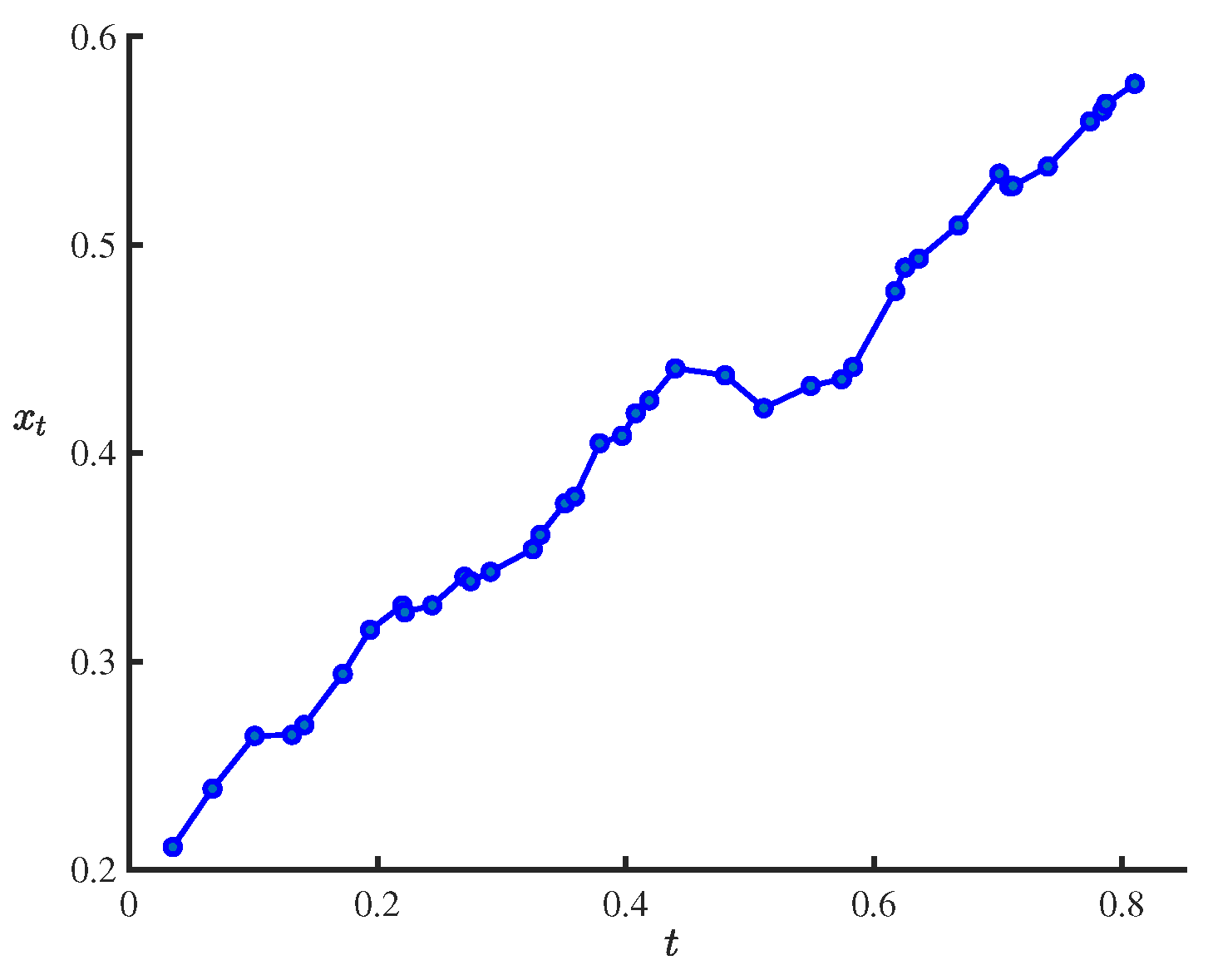
0.035	0.2109	0.067	0.2389	0.101	0.2643	0.131	0.2647
0.141	0.2695	0.172	0.2940	0.194	0.3152	0.220	0.3269
0.222	0.3236	0.244	0.3270	0.270	0.3407	0.275	0.3385
0.291	0.3430	0.325	0.3539	0.331	0.3608	0.351	0.3759
0.359	0.3792	0.379	0.4048	0.397	0.4083	0.408	0.4191
0.419	0.4253	0.440	0.4407	0.480	0.4374	0.511	0.4216
0.549	0.4323	0.574	0.4355	0.583	0.4413	0.617	0.4777
0.625	0.4891	0.636	0.4934	0.668	0.5093	0.701	0.5342
0.709	0.5283	0.712	0.5283	0.740	0.5376	0.774	0.5593
0.784	0.5642	0.787	0.5677	0.810	0.5773

and Figure 1).

Let us represent the observed time points in Table 1 as $t_1,t_2,\cdots ,t_{39}$, and the observed values of $X_t$ at these time points as

$$x_{t_1},x_{t_2},\cdots ,x_{t_{39}}.$$

Given a confidence level $\beta =0.95$, it follows from (9) that the $95\%$ confidence interval of the initial value is

$$\begin{array}{cc}\hfill {\mathcal{S}}_{\beta }=& \left[\underset{i=1}{\overset{39}{\bigvee }}\left(x_{t_i}-0.4769t_i-{\displaystyle \frac{\sqrt{3}\times 1.8493t_i}{\pi }}ln{\displaystyle \frac{1+0.95}{1-0.95}}\right),\right.\hfill \\ \hfill & \left.\underset{i=1}{\overset{39}{\bigwedge }}\left(x_{t_i}-0.4769t_i+{\displaystyle \frac{\sqrt{3}\times 1.8493t_i}{\pi }}ln{\displaystyle \frac{1+0.95}{1-0.95}}\right)\right],\hfill \end{array}$$

i.e.,

$${\mathcal{S}}_{\beta }=[0.0635,0.3250],$$

and the point estimation of the initial value is

$$\mu ={\displaystyle \frac{0.0635+0.3250}{2}}=0.19425$$

as can be established immediately.

Example 5. 

Suppose we have a set of observational data concerning the following linear uncertain differential equation starting with $t_0=0$:

$$\mathrm{d}{X}_t=0.2892X_t\mathrm{d}t+3.8493X_t\mathrm{d}{C}_t,$$

(as described in

Table 2. Observational data of Example 5.

${\mathit{t}}_{\mathit{i}}$	${\mathit{x}}_{{\mathit{t}}_{\mathit{i}}}$	${\mathit{t}}_{\mathit{i}}$	${\mathit{x}}_{{\mathit{t}}_{\mathit{i}}}$	${\mathit{t}}_{\mathit{i}}$	${\mathit{x}}_{{\mathit{t}}_{\mathit{i}}}$	${\mathit{t}}_{\mathit{i}}$	${\mathit{x}}_{{\mathit{t}}_{\mathit{i}}}$
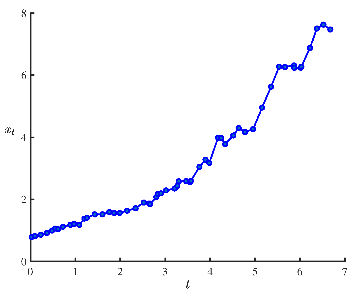
0.0250	0.7881	0.1000	0.8189	0.2250	0.8635	0.3650	0.9208
0.4800	0.9969	0.5500	1.0627	0.6100	1.0420	0.7200	1.1202
0.8850	1.1795	0.9650	1.2064	0.9700	1.2108	1.0850	1.1824
1.2000	1.3831	1.2550	1.4113	1.4300	1.5200	1.6000	1.5213
1.7550	1.5946	1.8600	1.5631	1.9850	1.5653	2.1500	1.6372
2.3400	1.7156	2.5200	1.8997	2.6450	1.8707	2.6600	1.8482
2.8000	2.0791	2.8350	2.1684	2.9000	2.1943	3.0150	2.2907
3.2100	2.3519	3.2700	2.4408	3.3000	2.5845	3.4650	2.5918
3.5500	2.5569	3.5700	2.5979	3.7600	3.0474	3.8950	3.2799
3.9800	3.1765	4.1750	3.9873	4.2450	3.9745	4.3350	3.7825
4.5150	4.0610	4.6350	4.2998	4.7750	4.1735	4.9550	4.2633
5.1550	4.9579	5.3550	5.6321	5.5350	6.2784	5.6650	6.2671
5.8650	6.3201	5.8700	6.2420	6.0150	6.2449	6.0300	6.2781
6.2200	6.8810	6.3750	7.5052	6.5200	7.6322	6.6750	7.4769

and Figure 2).

Let us represent the observed time points in Table 2 as $t_1,t_2,\cdots ,t_{56}$, and the observed values of $X_t$ at these time points as

$$x_{t_1},x_{t_2},\cdots ,x_{t_{56}}.$$

Given a confidence level $\beta =0.95$, it follows from (13) that the $95\%$ confidence interval of the initial value is

$$\begin{array}{cc}\hfill {\mathcal{S}}_{\beta }=& \left[exp\left(\underset{i=1}{\overset{56}{\bigvee }}\left(ln{x}_{t_i}-a{t}_i-{\displaystyle \frac{\sqrt{3}\times 3.8493t_i}{\pi }}ln{\displaystyle \frac{1+0.95}{1-0.95}}\right)\right)\right.\hfill \\ \hfill & \left.exp\left(\underset{i=1}{\overset{n}{\bigwedge }}\left(ln{x}_{t_i}-a{t}_i+{\displaystyle \frac{\sqrt{3}\times 3.8493t_i}{\pi }}ln{\displaystyle \frac{1+0.95}{1-0.95}}\right)\right)\right],\hfill \end{array}$$

i.e.,

$${\mathcal{S}}_{\beta }=[0.6442,0.9503],$$

and the point estimation of the initial value is

$$\mu ={\displaystyle \frac{0.6442+0.9503}{2}}=0.79725$$

as can be established immediately.

6. IPO Price Estimation in Stock Market

The IPO (Initial Public Offering) price of a stock, also known as the offering price or listing price, refers to the price at which a company sells shares to public investors when it first issues shares on the open market. This price is usually determined by a combination of the issuing company, underwriters (usually investment banks), and market conditions. IPO price is an important step in the process of listing a company, which not only reflects the market’s valuation of the company, but also affects the subsequent performance of the company in the market and investors’ confidence in the company. However, sometimes due to technical reasons, we cannot directly obtain the IPO price of a certain stock, in which case we need to estimate its IPO price according to the opening prices of the stock in the market.

6.1. Data Source

We collected the opening price data of EZVIZ Network. This was the first stock pertaining to smart homes, which the Science and Technology board listed on the Shanghai Stock Exchange on 28 December 2022. The data are from the second week of listing (3 January 2023) to 21 June 2024, and they are sorted into the weekly average opening price data, as shown in

Table 3. Weekly average opening price data of EZVIZ Network from 3 January 2023 to 21 June 2024.

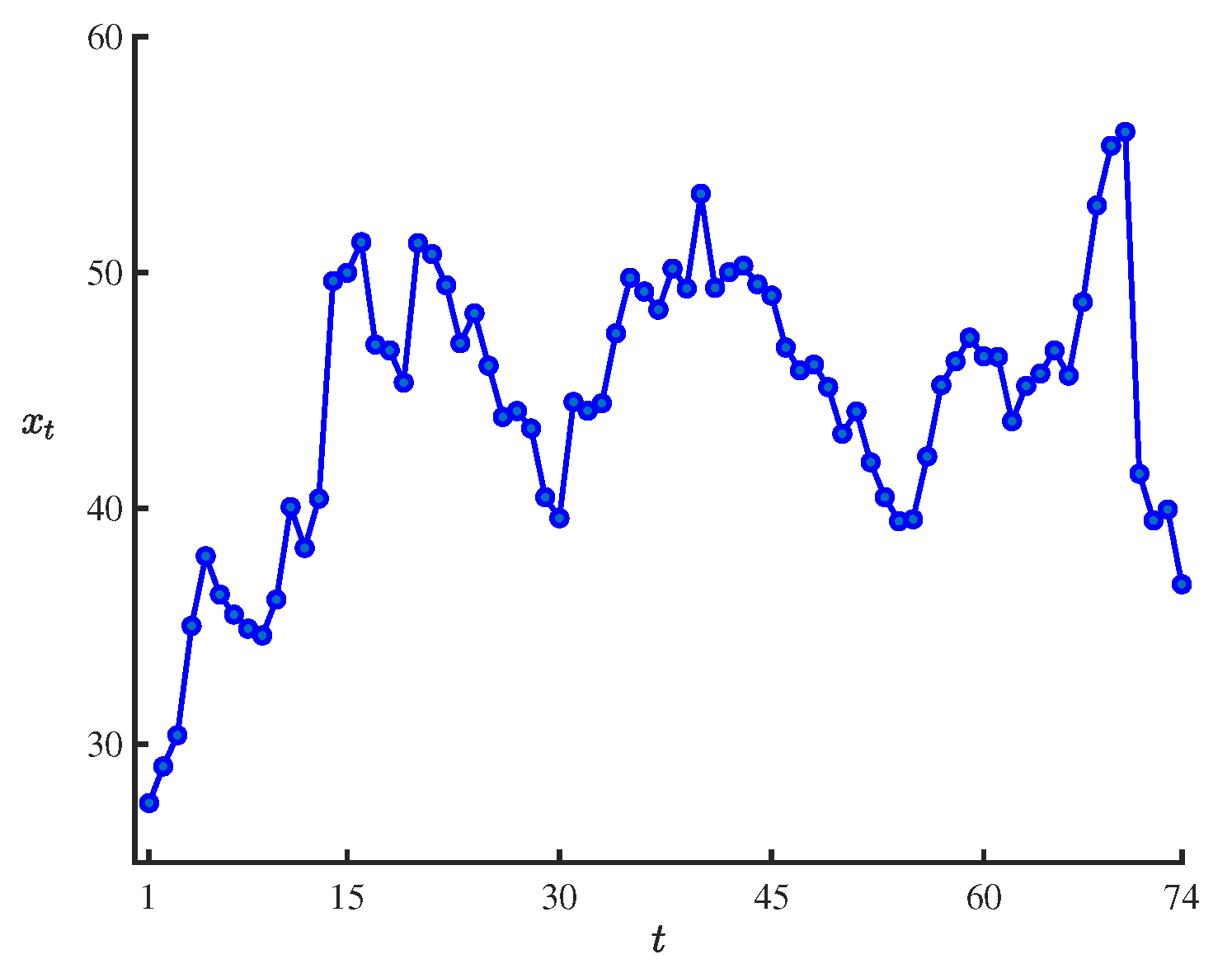
27.5225	29.0720	30.3960	35.0280	37.9820	36.3560	35.5040	34.9060	34.6220
36.1400	40.0660	38.3300	40.4225	49.6440	49.9920	51.2880	46.9500	46.7060
45.3400	51.2520	50.7860	49.4660	47.0040	48.2733	46.0500	43.8820	44.1300
43.3920	40.4820	39.5900	44.5140	44.1420	44.4600	47.4280	49.7780	49.1960
48.4260	50.1675	49.3260	53.3400	49.3540	50.0200	50.2900	49.5060	49.0240
46.8240	45.8560	46.1000	45.1460	43.1680	44.1125	41.9620	40.4820	39.4640
39.5460	42.2050	45.2280	46.2360	47.2440	46.4520	46.4280	43.7020	45.1967
45.7200	46.6980	45.6320	48.7500	52.8420	55.3740	55.9640	41.4760	39.4940
39.9575	36.7900

and Figure 3.

6.2. Uncertain Stock Prices Model

Let us denote the weeks from 3 January 2023 to 21 June 2024 by

$$t=1,2,\cdots ,74,$$

and denote the weekly average opening prices of EZVIZ Network for each week by

$$x_t,t=1,2,\cdots ,74.$$

According to the mean-reversion property of stock prices, we can use the uncertain mean-reversion differential equation

$$\mathrm{d}{X}_t=\left(m-a{X}_t\right)\mathrm{d}t+\sigma \mathrm{d}{C}_t,$$

to model the above opening price data.

For each index i with $2\le i\le 74$ and any given parameters m, a, and $\sigma$, we can calculate the ith residual of the above uncertain mean-reversion differential equation corresponding to the collected weekly average opening prices as

$${\epsilon }_i\left(m,a,\sigma \right)={\displaystyle \frac{1}{1+exp\left({\displaystyle \frac{\pi \left(\left(a{x}_{i-1}-m\right)exp\left(-a\right)+m-a{x}_i\right)}{\sqrt{3}\left|\sigma \right|\left(1-exp\left(-a\right)\right)}}\right)}}$$

by solving the following updated uncertain mean-reversion differential equation:

$$\mathrm{d}{X}_t=\left(m-a{X}_t\right)\mathrm{d}t+\sigma \mathrm{d}{C}_t,X_t{|}_{t=i-1}=x_{i-1}.$$

Then, we obtain 73 residuals as

$${\epsilon }_2\left(m,a,\sigma \right),{\epsilon }_3\left(m,a,\sigma \right),\cdots ,{\epsilon }_{74}\left(m,a,\sigma \right)$$

which is a set of samples of linear uncertain distribution $\mathcal{L}(0,1)$. Since there are three unknown parameters in the uncertain mean-reversion differential equation, the method of moment estimation requires us to ensure that the first three moments of the above samples are equal (or as close as possible) to the first three moments of linear uncertain distribution $\mathcal{L}(0,1)$. In other words, the moment estimations $\widehat{m}$, $\widehat{a}$, and $\widehat{\sigma }$ of unknown parameters can be used to solve the following system of equations:

$$\left\{\begin{array}{cc}{\displaystyle \frac{1}{73}\sum _{i=2}^{74}{\epsilon }_i\left(m,a,\sigma \right)=\frac{1}{2}}\hfill & \\ {\displaystyle \frac{1}{73}\sum _{i=2}^{74}{\epsilon }_i^2\left(m,a,\sigma \right)=\frac{1}{3}}\hfill & \\ {\displaystyle \frac{1}{73}\sum _{i=2}^{74}{\epsilon }_i^3\left(m,a,\sigma \right)=\frac{1}{4}}\hfill \end{array}\right.$$

The parameters are as follows:

$$\widehat{m}=17.4862,\widehat{a}=0.3898,\widehat{\sigma }=3.3616.$$

Thus, we obtain an estimated uncertain stock prices model as follows:

$$\begin{array}{c}\hfill \mathrm{d}{X}_t=\left(17.4862-0.3898X_t\right)\mathrm{d}t+3.3616\mathrm{d}{C}_t.\end{array}$$

(19)

6.3. IPO Price Estimation

Next, we estimate the weekly average opening price of the first week of EZVIZ Network stock issuance according to the weekly average opening price data collected in Table 3 and Figure 3. Since the second week is set to time 1, we set the initial time (the first week) to time 0.

Given a confidence level $\beta =0.95$, it follows from (17) that the $95\%$ confidence interval of the IPO Price is

$$\begin{array}{cc}\hfill {\mathcal{S}}_{\beta }=& \left[\underset{i=1}{\overset{74}{\bigvee }}\left({\displaystyle \frac{17.4862}{0.3898}}+exp\left(0.3898i\right)\left(x_i-{\displaystyle \frac{17.4862}{0.3898}}\right.\right.\right.\hfill \\ \hfill & \left.\left.-{\displaystyle \frac{1-exp\left(-0.3898i\right)}{0.3898}}{\displaystyle \frac{\sqrt{3}\times 3.3616}{\pi }}ln{\displaystyle \frac{1+0.95}{1-0.95}}\right)\right),\hfill \\ \hfill & \underset{i=1}{\overset{74}{\bigwedge }}\left({\displaystyle \frac{17.4862}{0.3898}}+exp\left(0.3898i\right)\left(x_i-{\displaystyle \frac{17.4862}{0.3898}}\right.\right.\hfill \\ \hfill & \left.\left.\left.+{\displaystyle \frac{1-exp\left(-0.3898i\right)}{0.3898}}{\displaystyle \frac{\sqrt{3}\times 3.3616}{\pi }}ln{\displaystyle \frac{1+0.95}{1-0.95}}\right)\right)\right],\hfill \end{array}$$

i.e.,

$${\mathcal{S}}_{\beta }=[10.9559,27.5628],$$

and the point estimation of the IPO Price is

$$\mu ={\displaystyle \frac{10.9559+27.5628}{2}}=19.25935$$

as can be derived immediately.

7. Conclusions

In order to estimate the initial value of uncertain differential equations, this paper studied the confidence interval and point estimation of the initial value of uncertain differential equations based on the residuals corresponding to observed data, and provided a numerical algorithm to calculate the initial value estimation numerically. Further, specific confidence intervals and point estimations for the initial values of uncertain differential equations such as linear, exponential, and mean-reversion equations were given. Finally, two numerical examples and an empirical study were provided to illustrate the application of the proposed method in practice. Therefore, this study provides an effective solution to the initial value estimation problem of uncertain differential equations, and future studies can apply the method to more complex uncertain situations, including high-order uncertain differential equations, multi-factor uncertain differential equations, delayed uncertain differential equations, and high-dimensional uncertain differential equations.

References

- Kolmogorov, A. Grundbegriffe der Wahrscheinlichkeitsrechnung; Springer: Berlin/Heidelberg, Germany, 1933. [Google Scholar]
- Itô, K. On Stochastic Differential Equations; American Mathematical Society: Providence, RI, USA, 1951. [Google Scholar]
- Kloeden, P.; Platen, E. Stochastic Differential Equations; Springer: Berlin/Heidelberg, Germany, 1992. [Google Scholar]
- Oksendal, B. Stochastic Differential Equations: An Introduction with Applications; Springer Science & Business Media: Berlin/Heidelberg, Germany, 2013. [Google Scholar]
- Higham, D.; Kloeden, P. An Introduction to the Numerical Simulation of Stochastic Differential Equations; Society for Industrial and Applied Mathematics: Philadelphia, PA, USA, 2021. [Google Scholar]
- Ye, T.; Liu, B. Uncertain significance test for regression coefficients with application to regional economic analysis. Commun. Stat.-Theory Methods 2023, 52, 7271–7288. [Google Scholar] [CrossRef]
- Jia, L.; Li, D.; Guo, F.; Zhang, B. Knock-in options of mean-reverting stock model with floating interest rate in uncertain environment. Int. J. Gen. Syst. 2024, 53, 331–351. [Google Scholar] [CrossRef]
- Liu, Z. Uncertain growth model for the cumulative number of COVID-19 infections in China. Fuzzy Optim. Decis. Mak. 2021, 20, 229–242. [Google Scholar] [CrossRef]
- Yang, L. Analysis of death toll from COVID-19 in China with uncertain time series and uncertain regression analysis. J. Uncertain Syst. 2022, 15, 2243007. [Google Scholar] [CrossRef]
- Ding, C.; Ye, T. Uncertain logistic growth model for confirmed COVID-19 cases in Brazil. J. Uncertain Syst. 2022, 15, 2243008. [Google Scholar] [CrossRef]
- Xie, J.; Lio, W. Uncertain nonlinear time series analysis with applications to motion analysis and epidemic spreading. Fuzzy Optim. Decis. Mak. 2024, 23, 279–294. [Google Scholar] [CrossRef]
- Liu, B. Fuzzy process, hybrid process and uncertain process. J. Uncertain Syst. 2008, 2, 3–16. [Google Scholar]
- Liu, B. Uncertainty Theory, 2nd ed.; Springer: Berlin/Heidelberg, Germany, 2007. [Google Scholar]
- Liu, B. Some research problems in uncertainty theory. J. Uncertain Syst. 2009, 3, 3–10. [Google Scholar]
- Chen, X.; Liu, B. Existence and uniqueness theorem for uncertain differential equations. Fuzzy Optim. Decis. Mak. 2010, 9, 69–81. [Google Scholar] [CrossRef]
- Yao, K.; Gao, J.; Gao, Y. Some stability theorems of uncertain differential equation. Fuzzy Optim. Decis. Mak. 2013, 12, 3–13. [Google Scholar] [CrossRef]
- Sheng, Y.; Wang, C. Stability in the p-th moment for uncertain differential equation. J. Intell. Fuzzy Syst. 2014, 26, 1263–1271. [Google Scholar] [CrossRef]
- Yao, K.; Ke, H.; Sheng, Y. Stability in mean for uncertain differential equation. Fuzzy Optim. Decis. Mak. 2015, 14, 365–379. [Google Scholar] [CrossRef]
- Yang, X.; Ni, Y.; Zhang, Y. Stability in inverse distribution for uncertain differential equations. J. Intell. Fuzzy Syst. 2017, 32, 2051–2059. [Google Scholar] [CrossRef]
- Yao, K.; Chen, X. A numerical method for solving uncertain differential equations. J. Intell. Fuzzy Syst. 2013, 25, 825–832. [Google Scholar] [CrossRef]
- Yang, X.; Shen, Y. Runge-Kutta method for solving uncertain differential equations. J. Uncertain Anal. Appl. 2015, 3, 17. [Google Scholar] [CrossRef]
- Yang, X.; Ralescu, D. Adams method for solving uncertain differential equations. Appl. Math. Comput. 2015, 270, 993–1003. [Google Scholar] [CrossRef]
- Gao, R. Milne method for solving uncertain differential equations. Appl. Math. Comput. 2016, 274, 774–785. [Google Scholar] [CrossRef]
- Yao, K.; Liu, B. Parameter estimation in uncertain differential equations. Fuzzy Optim. Decis. Mak. 2020, 19, 1–12. [Google Scholar] [CrossRef]
- Liu, Y.; Liu, B. Estimating unknown parameters in uncertain differential equation by maximum likelihood estimation. Soft Comput. 2022, 26, 2773–2780. [Google Scholar] [CrossRef]
- Liu, Y.; Liu, B. Residual analysis and parameter estimation of uncertain differential equations. Fuzzy Optim. Decis. Mak. 2022, 21, 513–530. [Google Scholar] [CrossRef]
- Liu, Y.; Liu, B. A modified uncertain maximum likelihood estimation with applications in uncertain statistics. Commun. Stat.-Theory Methods 2023, 53, 6649–6670. [Google Scholar] [CrossRef]
- Liu, Y.; Liu, B. Estimation of uncertainty distribution function by the principle of least squares. Commun. Stat.-Theory Methods 2023, 53, 7624–7641. [Google Scholar] [CrossRef]
- Lio, W.; Liu, B. Initial value estimation of uncertain differential equations and zero-day of COVID-19 spread in China. Fuzzy Optim. Decis. Mak. 2021, 20, 177–188. [Google Scholar] [CrossRef]