On the Global Dynamics of a Fourth-Order Riccati-Type Exponential Fuzzy Difference Equation

Abstract

Fuzzy systems play a crucial role in emerging fields such as artificial intelligence, machine learning, and computer science, drawing significant research interest in fuzzy difference equations. Inspired by this, we analyze the dynamic properties of a fourth-order exponential Riccati-type fuzzy difference equation. The study is further extended to a system of fourth-order fuzzy difference equations. We investigate the boundedness, as well as the local and global stability, of positive solutions. To support the theoretical findings, numerical examples are presented along with graphical and tabular representations.

1. Introduction and Motivation

A need for mathematical models explaining real-life circumstances has led to the study of non-linear differential equations in computer science, ecology, economics, probability theories, biology, and psychology. A current imbalance in mathematical design for computer simulation and experimentation seems to be well suited to the rapid development of computer-oriented computation techniques (see [1,2,3,4,5]). It is true that we have to deal with many real-life practical issues that remain unresolved if we use the differential equation model. Fuzzy set theory serves as an effective framework for managing uncertainty and addressing imprecise outcomes in mathematical models. In a fuzzy difference equation (FDE), initial values are expressed as fuzzy numbers (FNs), while parameters are considered fixed constants. The dynamics of parametric FDEs can be studied by examining corresponding families of parametric ordinary differential equations, extending results through fuzzy modeling techniques.

Deeba et al. [6] introduced a first-degree difference equation (DE), incorporating historical context, as follows:

$$\begin{array}{c}\hfill D_{t+1}=a_1{D}_t+b_1,\end{array}$$

where $t\in \mathbb{W}$, $D_t$, $a_1$, and $b_1$ are from a genetic population dataset and appear as FN sequences in genetic studies.

Subsequently, Deeba and de Korvin [7] explored second-order linear fuzzy equations as follows:

$$\begin{array}{c}\hfill E_{n+1}=E_n-g_1{h}_1{E}_{n-1}+p_1,\end{array}$$

where $n\in \mathbb{W}$ and $E_n$ represents a sequence of nonzero FNs, and $g_1$, $h_1$, and $p_1$ are fuzzy parameters. This equation has been applied in modeling CO₂ concentration in human blood through a linearized version of a nonlinear FDE.

Mondal et al. [8] utilized the multiplier method to investigate second-order linear FDEs. Khastan [9] examined the following fuzzy logistic difference equation:

$$x_{n+1}=\beta x_n(1-x_n),$$

where $x_n$ and $\beta$ are positive FNs; he thus derived results on global solution behavior.

Papaschinopoulos and Papadopoulos [10] applied Zadeh’s extension principle to analyze the global dynamics of an FDE:

$$\begin{array}{c}\hfill u_{n+1}=A+{\displaystyle \frac{B}{u_n}},\end{array}$$

where A and B are positive FNs. Further, they examined another FDE given by the following [11]:

$$\begin{array}{c}\hfill u_{n+1}=A+{\displaystyle \frac{u_n}{u_{n-m}}},\end{array}$$

where $m\in \mathbb{N}$, $n\in \mathbb{W}$, and A is a positive FN.

Several researchers have since extended these approaches to study various FDEs, leading to numerous insights. For further reference, readers may consult [4,12,13,14,15,16,17,18].

In set-valued and fuzzy analysis, Minkowski additions and multiplications are generally not invertible. However, inversion in multiplication and addition plays a crucial role in interval and fuzzy analysis, particularly in solving equations, interval computations, and fuzzy difference equations (FDEs). To address these challenges, Stefanini [19] introduced a generalized division method for fuzzy numbers (FNs), known as g-division. One of the key benefits of g-division is its ability to enhance precision in fuzzy solutions by reducing the length of support intervals. Zhang et al. [16] applied g-division to examine the global behavior of third-order rational FDEs, a model that was later revisited by Khastan and Alijani [20]. The application of g-division in FDEs has been a topic of increasing interest in recent studies [21,22].

Papaschinopoulos and Stefanidou [23] investigated the uniqueness, persistence, existence, and boundedness of nonzero solutions in the following FDE:

$$\begin{array}{c}\hfill D_{n+1}=\sum _{m=0}^j{{\displaystyle \frac{A_m}{D_{n-m}^{q_m}}}}^{\prime }\end{array}$$

where, $j\in N$, $n=0,1,2,\dots$, and the coefficients $A_m$, where $m\in \{0,1,2,\dots ,j\}$, are nonzero FNs. The parameters $q_m$ are nonzero real constants, while the initial values $D_m$ for $m\in \{-j,-j+1,\dots ,0\}$ are nonzero fuzzy numbers.

Additionally, Papaschinopoulos and Stefanidou [23] explored the periodicity properties of a max-type FDE:

$$\begin{array}{c}\hfill S_{j+1}=max\left[{\displaystyle \frac{B_0}{S_{j-m}}},{\displaystyle \frac{B_1}{S_{j-n}}}\right],\end{array}$$

where m and n are positive integers, $B_0$ and $B_1$ are nonzero FNs, and the initial values $S_j$ for $j\in \{-a,-a+1,\dots ,-1\}$ (with $a=max\{m,n\}$) are also nonzero fuzzy numbers.

Zhang et al. [17] explained the existence and asymptotic properties of nonzero solutions in a nonlinear fuzzy difference equation (FDE):

$$\begin{array}{c}\hfill z_{m+1}={\displaystyle \frac{A_1{z}_m+z_{m-1}}{B_1+z_{m-1}}},m\in W\end{array}$$

where $\left\{z_m\right\}$ represents a sequence of nonzero fuzzy numbers (FNs), and $A_1$ and $B_1$ are parameters with initial conditions $z_{-1}$ and $z_0$ that are nonzero FNs. Building on this, Zhang et al. [17] further examined the asymptotic behavior, boundedness, and existence of nonzero solutions in a first-degree Riccati difference equation:

$$\begin{array}{c}\hfill z_{t+1}={\displaystyle \frac{C_1+z_t}{D_1+z_t}},t=0,1,2,3,\dots \end{array}$$

where $z_t$, $C_1$, and $D_1$ are nonzero FNs.

The study of third-degree rational FDEs was extended in [18], where Zhang et al. analyzed the following model:

$$\begin{array}{c}\hfill t_{m+1}={\displaystyle \frac{B_{1}t+t_{m-1}}{t_{m-1}{t}_{m-2}}},m=0,1,2,3,\dots \end{array}$$

with initial conditions $t_0$, $t_{-1}$, and $t_{-2}$ as nonzero FNs, while $B_1$ remains a parameter.

Khastan [21] explored the global behavior, uniqueness, and persistence of solutions for the FDE:

$$\begin{array}{c}\hfill y_{m+1}-q=b{y}_m,m=0,1,2,\dots \end{array}$$

where $\left\{y_m\right\}$ is a sequence of nonzero FNs, with $y_0$, q, and b being nonzero fuzzy parameters. The general qualitative behavior of fuzzy difference equations was analyzed in [24], while [25] investigated the dynamical properties of a k-order FDE. However, both studies focused on relatively simple fuzzy difference equations.

More recently, Zhang et al. [26] introduced the notion of boundedness, convergence rate, and characteristics of nonnegative solutions in a second-order exponential-type FDE:

$$\begin{array}{c}\hfill z_{m+1}={\displaystyle \frac{A+B{e}^{-z_m}}{C+z_{m-1}}},m=0,1,2,\dots \end{array}$$

where $m\in \mathbb{W}$, $z_{-1}$ and $z_0$ are initial conditions, and A, B, and C all are positive FNs. Furthermore, a second-order system of exponential-type fuzzy difference equations was explored in [27].

Motivated by these studies, this paper focuses on the dynamic behavior of a fourth-order Riccati-type exponential FDE and extends the analysis to a system of such equations. The objective is to establish the existence, uniqueness, and global behavior of solutions by employing the g-division method for FN. We adopt the approach outlined in [21] and apply our findings to discrete-time dynamical models incorporating fuzzy uncertainties.

This paper uniquely addresses gaps in prior research by tackling limitations in the analysis of fourth-order Riccati-type exponential fuzzy difference equations, which have been overlooked in previous studies. Unlike existing work, it focuses on a Riccati-type exponential fuzzy difference equation to analyze the dynamical behavior of this type of equation, providing fresh insights into its behavior and solutions. This contribution helps to advance understanding in the field of fuzzy difference equations and suggests new directions for future research.

The remainder of this paper is structured as follows. Section 2 discusses preliminaries and known results. Section 3 explores the existence and global dynamics of a fourth-order Riccati-type exponential FDE based on specific characterization theorems. Several numerical examples illustrating our results are presented in Section 4. Lastly, Section 5 provides a summary of key findings and suggests potential directions for future research.

2. Preliminaries

In this section, we review key definitions and results that are essential for the remainder of the paper. For a more detailed discussion, see [1,19,28].

Definition 1

([28]). A fuzzy number (FN) is a function $u:\mathbb{R}\to [0,1]$ that satisfies the following properties:

(i) 

**Normality:** There exists some $k_1\in \mathbb{R}$ such that $u\left(k_1\right)=1$.

(ii) 

**Fuzzy Convexity:** For all $0\le t\le 1$ and $k_1,k_2\in \mathbb{R}$,

$$u(t{k}_1+(1-t)k_2)\ge min\{u\left(k_1\right),u\left(k_2\right)\}.$$

(iii) 

**Upper Semicontinuity:** The function u is upper semicontinuous on $\mathbb{R}$.

(iv) 

**Compact Support:** The support of u, denoted as

$$\mathit{supp}\left(u\right)=\mathit{cl}\{k\in \mathbb{R}:u(k)>0\},$$

is a compact set.

For $0\le \sigma \le 1$, the corresponding σ-cut of an FN u is given by

$${\left[u\right]}_{\sigma }=\{k\in \mathbb{R}\mid u\left(k\right)\ge \sigma \}.$$

For $\sigma =0$, it is defined as

$${\left[u\right]}_0=\mathit{cl}\{k\in \mathbb{R}\mid u\left(k\right)>0\}.$$

It follows that ${\left[u\right]}_0=\mathit{supp}\left(u\right)$.

A fuzzy number u is said to be positive if its support is contained in the interval $(0,\infty )$.

A fuzzy number can also be represented as an ordered pair of functions.

Theorem 1

([28]). Let $u_l,u_r:[0,1]\to \mathbb{R}$ be functions satisfying the following properties:

(i) 

The function $u_l$ is LC (i.e., left-continuous) on $(0,1]$, RC (i.e., right-continuous) at 0, bounded, and non-decreasing.

(ii) 

The function $u_r$ is LC (i.e., left-continuous) on $(0,1]$, RC (i.e., right-continuous) at 0, bounded, and non-increasing.

(iii) 

$u_l\left(1\right)\le u_r\left(1\right)$.

Then, a fuzzy number u exists such that $u_l\left(\sigma \right)$ and $u_r\left(\sigma \right)$ represent the endpoints of its σ-cut ${\left[u\right]}_{\sigma }$.

Define ${\mathbb{R}}_f=\{u\mid {\left[u\right]}_{\sigma }=[u_l\left(\sigma \right),u_r\left(\sigma \right)]\mathrm{for}\mathrm{all}\sigma \in [0,1]\}$ as the space of all fuzzy numbers, and let ${\mathbb{R}}_f^{+}$ denote the subset of positive fuzzy numbers.

Definition 2

([28]). A triangular FN is a triplet $D=(\eta ,\varphi ,\xi )$ with the membership function $D:\mathbb{R}\to [0,1]$ given by

$$D\left(k\right)=\left\{\begin{array}{cc}{\displaystyle \frac{k-\eta }{\varphi -\eta }},\hfill & \mathit{if}k\in [\eta ,\varphi ),\hfill \\ 1,\hfill & \mathit{if}k=\varphi ,\hfill \\ {\displaystyle \frac{\xi -k}{\xi -\varphi }},\hfill & \mathit{if}k\in (\varphi ,\xi ],\hfill \\ 0,\hfill & \mathit{if}k\notin [\eta ,\varphi ].\hfill \end{array}\right.$$

(1)

The σ-cuts of $D=(\eta ,\varphi ,\xi )$ are defined by ${\left[d\right]}_{\sigma }=[\eta +\sigma (\varphi -\eta ),\xi -\sigma (\xi -\varphi )]$ for $0\le \sigma \le 1$. Clearly, the ${\left[d\right]}_{\sigma }$ parts are closed.

Definition 3

([20]). Assume that $a,b\in {\mathbb{R}}_f$. Then, we define the metric on the FN space as follows:

$$D(a,b)=\underset{\sigma \in [0,1]}{sup}max\left\{\right|a_l\left(\sigma \right)-b_l\left(\sigma \right)|,|a_r\left(\sigma \right)-b_r\left(\sigma \right)\left|\right\}.$$

(2)

Definition 4.

Assume that $\eta ,\varphi \in {\mathbb{R}}_f$ and $\lambda \in \mathbb{R}$. Then, $\eta +\varphi$, $\eta -\varphi$, $\lambda \eta$, $\eta \varphi$, ${\displaystyle \frac{\eta }{\varphi }}$ is defined by the following:

(i) 

${[\eta +\varphi ]}_{\sigma }=[{\eta }_l\left(\sigma \right)+{\varphi }_l\left(\sigma \right),{\eta }_r\left(\sigma \right)+{\varphi }_r\left(\sigma \right)]$ for $0\le \sigma \le 1$.

(ii) 

${[\eta -\varphi ]}_{\sigma }=[{\eta }_l\left(\sigma \right)-{\varphi }_l\left(\sigma \right),{\eta }_r\left(\sigma \right)-{\varphi }_r\left(\sigma \right)]$ for $0\le \sigma \le 1$.

(iii) 

${\left[\lambda \eta \right]}_{\sigma }=\left\{\begin{array}{cc}[\lambda {\eta }_l\left(\sigma \right),\lambda {\eta }_r\left(\sigma \right)],\hfill & \mathit{if}\lambda \ge 0,\hfill \\ [\lambda {\eta }_r\left(\sigma \right),\lambda {\eta }_l\left(\sigma \right)],\hfill & \mathit{if}\lambda <0,\hfill \end{array}\right.$ for $\sigma \in [0,1]$.

(iv) 

$\begin{array}{c}{\left[\eta \varphi \right]}_{\sigma }=[min\{{\eta }_l\left(\sigma \right){\varphi }_l\left(\sigma \right),{\eta }_r\left(\sigma \right){\varphi }_l\left(\sigma \right),{\eta }_l\left(\sigma \right){\varphi }_r\left(\sigma \right),{\eta }_r\left(\sigma \right){\varphi }_r\left(\sigma \right)\},\hfill \\ max\{{\eta }_l\left(\sigma \right){\varphi }_l\left(\sigma \right),{\eta }_r\left(\sigma \right){\varphi }_l\left(\sigma \right),{\eta }_l\left(\sigma \right){\varphi }_r\left(\sigma \right),{\eta }_r\left(\sigma \right){\varphi }_r\left(\sigma \right)\}]\mathit{for}\sigma \in [0,1].\hfill \end{array}$

(v) 

${\left[{\displaystyle \frac{\eta }{\varphi }}\right]}_{\sigma }=\left[min\left\{{\displaystyle \frac{{\eta }_l\left(\sigma \right)}{{\varphi }_l\left(\sigma \right)}},{\displaystyle \frac{{\eta }_r\left(\sigma \right)}{{\varphi }_l\left(\sigma \right)}},{\displaystyle \frac{{\eta }_l\left(\sigma \right)}{{\varphi }_r\left(\sigma \right)}},{\displaystyle \frac{{\eta }_r\left(\sigma \right)}{{\varphi }_r\left(\sigma \right)}}\right\},max\left\{{\displaystyle \frac{{\eta }_l\left(\sigma \right)}{{\varphi }_l\left(\sigma \right)}},{\displaystyle \frac{{\eta }_r\left(\sigma \right)}{{\varphi }_l\left(\sigma \right)}},{\displaystyle \frac{{\eta }_l\left(\sigma \right)}{{\varphi }_r\left(\sigma \right)}},{\displaystyle \frac{{\eta }_r\left(\sigma \right)}{{\varphi }_r\left(\sigma \right)}}\right\}\right]$ for $0\le \sigma \le 1$.

Theorem 2

(Stacking Theorem, [28]). If $u\in {\mathbb{R}}_f$, then

(i) 

${\left[u\right]}_{\sigma }$ is a closed for any $0\le \sigma \le 1$.

(ii) 

If ${\sigma }_1,{\sigma }_2\in [0,1]$ and ${\sigma }_1\le {\sigma }_2$, then ${\left[u\right]}_{{\sigma }_2}\subset {\left[u\right]}_{{\sigma }_1}$.

(iii) 

If we compute the convergence rate for any sequence ${\sigma }_n$ from below to 0, we have ${\left[u\right]}_{\sigma }={\bigcap }_{n=1}^{\infty }{\left[u\right]}_{{\sigma }_n}$.

(iv) 

If we compute the convergence rate for any sequence ${\sigma }_n$ from above to 0, we have ${\left[u\right]}_0=cl\left({\bigcup }_{n=1}^{\infty }{\left[u\right]}_{{\sigma }_n}\right)$.

Definition 5

([19]). Let $\eta ,\varphi \in {\mathbb{R}}_f$ have σ cuts, ${\left[\eta \right]}_{\sigma }=[{\eta }_l\left(\sigma \right),{\eta }_r\left(\sigma \right)]$, ${\left[\varphi \right]}_{\sigma }=[{\varphi }_l\left(\sigma \right),{\varphi }_r\left(\sigma \right)]$, with $0\notin {\left[\varphi \right]}_{\sigma }$ for all $0\le \sigma \le 1$. The g-division (${÷}_g$) of η and ϕ is an operation that calculates $\xi =\eta {÷}_g\varphi$ having σ-cuts ${\left[\xi \right]}_{\sigma }=[{\xi }_l\left(\sigma \right),{\xi }_r\left(\sigma \right)]$ defined by

$${\left[\xi \right]}_{\sigma }={\left[\eta \right]}_{\sigma }{÷}_g{\left[\varphi \right]}_{\sigma }\iff \left\{\begin{array}{c}{\left[\eta \right]}_{\sigma }={\left[\varphi \right]}_{\sigma }{\left[\xi \right]}_{\sigma }\hfill \\ or\hfill \\ {\left[\varphi \right]}_{\sigma }={\left[\eta \right]}_{\sigma }{\left[\xi \right]}_{\sigma }^{-1},\hfill \end{array}\right.$$

(3)

provided that ξ is a proper FN, where ${\left[\xi \right]}_{\sigma }^{-1}=[{\displaystyle \frac{1}{{\xi }_r\left(\sigma \right)}},{\displaystyle \frac{1}{{\xi }_l\left(\sigma \right)}}]$ and standard interval arithmetic is used for multiplications between intervals.

Remark 1.

Let $\eta ,\varphi \in {\mathbb{R}}_f^{+}$. If $\eta {÷}_g\varphi =\xi \in {\mathbb{R}}_f$ exists, then we have the following two cases:

• If ${\eta }_l\left(\sigma \right){\varphi }_r\left(\sigma \right)\le {\eta }_r\left(\sigma \right){\varphi }_l\left(\sigma \right)$ for $0\le \sigma \le 1$, then ${\xi }_l\left(\sigma \right)={\eta }_l\left(\sigma \right)/{\varphi }_l\left(\sigma \right)$, ${\xi }_r\left(\sigma \right)={\eta }_r\left(\sigma \right)/{\varphi }_r\left(\sigma \right)$ and the first case in (3) is satisfied.
• If ${\eta }_l\left(\sigma \right){\varphi }_r\left(\sigma \right)\ge {\eta }_r\left(\sigma \right){\varphi }_l\left(\sigma \right)$ for $\sigma \in [0,1]$, then ${\xi }_l\left(\sigma \right)={\eta }_r\left(\sigma \right)/{\varphi }_r\left(\sigma \right)$, ${\xi }_r\left(\sigma \right)={\eta }_l\left(\sigma \right)/{\varphi }_l\left(\sigma \right)$ and the second case in (3) is satisfied.

Definition 6.

A sequence $x_n\in {\mathbb{R}}_f^{+}$

• Persists if there exists $\lambda >0$ such that $supp\left(x_n\right)\subset [\lambda ,\infty )$;
• Is bounded if there exists $\delta >0$ such that $supp\left(x_n\right)\subset (0,\delta ]$;
• If $\lambda ,\delta >0$, then the function is bounded and persists s.t $sup\left(x_n\right)\subset [\lambda ,\delta ]$.

Definition 7.

If $x_n$ satisfies (6), it is considered as the positive fuzzy solution of (6). A positive FN k is referred to as a +ve equilibrium of (6) if

$$k={\displaystyle \frac{\sigma +\beta e^{-k}}{A+k}}.$$

(4)

Definition 8.

Consider a sequence of +ve FN $k_n$ and $k\in {\mathbb{R}}_f^{+}$. Then, $k_n\to k$ as $n\to \infty$ if ${\lim }_{n\to \infty }D(k_n,k)=0$.

Theorem 3

([29]). Let us consider the FDE problem

$$m_{i+1}=g(m_i,i)$$

(5)

with the initial value $m_0$, and where $g:{\mathbb{R}}_f\times Z_{\ge 0}\to {\mathbb{R}}_f$ is such that the following hold:

(1) 

The parametric shapes of that function are

$${\left[g(m_i,i)\right]}_{\sigma }=[\underline{g}(m_{i,l}\left(\sigma \right),m_{i,r}\left(\sigma \right),i,\sigma ),\overline{g}(m_{i,l}\left(\sigma \right),m_{i,r}\left(\sigma \right),i,\sigma )];$$

(2) 

The functions $\underline{g}(m_{i,l}\left(\sigma \right),m_{i,r}\left(\sigma \right),i,\sigma )$ and $\overline{g}(m_{i,l}\left(\sigma \right),m_{i,r}\left(\sigma \right),i,\sigma )$ are taken as continuous functions if for every ${ϵ}_1>0$, there exists ${\delta }_1>0$ s.t

$${\forall }_{\sigma \in [0,1]}|\underline{g}(m_{i,l}\left(\sigma \right),m_{i,r}\left(\sigma \right),i)-\overline{g}(m_{i_1,l}\left(\sigma \right),m_{i_1,r}\left(\sigma \right),i_1)|<{ϵ}_1$$

with $\left|\right|(m_{i,l}\left(\sigma \right),m_{i,r}\left(\sigma \right),i)-(m_{i_1,l}\left(\sigma \right),m_{i_1,r}\left(\sigma \right),i_1)|<{\delta }_1$, and for every ${ϵ}_2>0$, there exists ${\delta }_2>0$ such that

$${\forall }_{\sigma \in [0,1]}|\underline{g}(m_{i,l}\left(\sigma \right),m_{i,r}\left(\sigma \right),i,\sigma )-\overline{g}(m_{i_2,l}\left(\sigma \right),m_{i_2,r}\left(\sigma \right),i_2)|<{ϵ}_2$$

with $\left|\right|(m_{i,l}\left(\sigma \right),m_{i,r}\left(\sigma \right),i)-(m_{i_2,l}\left(\sigma \right),m_{i_2,r}\left(\sigma \right),i_2)|<{\delta }_2$.

Then, the single DE (5) can be converted to a system of two DEs as follows:

$$\begin{array}{cc}\hfill m_{i+1,l}\left(\sigma \right)& =\underline{g}(m_{i,l}\left(\sigma \right),m_{i,r}\left(\sigma \right),i,\sigma ),\hfill \\ \hfill m_{i+1,r}\left(\sigma \right)& =\overline{g}(m_{i,l}\left(\sigma \right),m_{i,r}\left(\sigma \right),i,\sigma ),\hfill \end{array}$$

with initial values $m_{0,l}\left(\sigma \right)$, $m_{0,r}\left(\sigma \right)$.

In this paper, we consider an exponential FDE; so, by the characterization theorem, this equation can be broken up into a system of two crisp DEs.

3. Main Results

In this section, we propose the following Riccati-type exponential FDE of the fourth order:

$$z_{m+1}={\displaystyle \frac{D+E{e}^{-z_{m-2}}}{F+z_{m-3}}},m=0,1,2,\dots$$

(6)

where $\left\{z_m\right\}$ is a sequence of +ve FNs, and D, E, and F are +ve FNs with $t_{-2}$, $t_{-1}$, and $t_0$ as the initial conditions. To investigate the existence and global behavior of this equation, we first prove the following lemma.

Lemma 1

([11]). Let k be a function which is continuous from ${\mathbb{R}}_{+}\times {\mathbb{R}}_{+}\times {\mathbb{R}}_{+}$ to ${\mathbb{R}}_{+}$ and $D,E,F\in {\mathbb{R}}_f$. Then,

$$\begin{array}{c}\hfill {\left[k(D,E,F)\right]}_{\sigma }=k({\left[D\right]}_{\sigma },{\left[E\right]}_{\sigma },{\left[F\right]}_{\sigma }),\sigma \in [0,1].\end{array}$$

(7)

Theorem 4.

Consider Equation (6), in which $t_i$ is the sequence of positive FNs, $D,E,F\in {\mathbb{R}}_f^{+}$ are non-zero constants, and $t_{-3},t_{-2},t_{-1},t_0\in {\mathbb{R}}_f^{+}$ are the initial conditions. Then, there exists a unique non-zero solution $t_i$ of Equation (6) with initial conditions $t_{-3},t_{-2},t_{-1}$, and $t_0$.

Proof. 

The steps of this proof follow from [16] (Theorem 3.1). Suppose we have a sequence of FNs $t_i$ which satisfies (6) with the initial conditions $t_{-3},t_{-2},t_{-1}$, and $t_0$. Now, consider the $\sigma$-cut for $0\le \sigma \le 1$

$${\left[D\right]}_{\sigma }=[D_{l,\sigma },D_{r,\sigma }],{\left[E\right]}_{\sigma }=[E_{l,\sigma },E_{r,\sigma }],{\left[F\right]}_{\sigma }=[F_{l,\sigma },F_{r,\sigma }],$$

(8)

and

$${\left[t_i\right]}_{\sigma }=[L_{i,\sigma },R_{i,\sigma }],i=-3,-2,-1,\dots .$$

(9)

From Lemma 1, it follows that

$$\begin{array}{cc}\hfill {\left[t_{i+1}\right]}_{\sigma }& =[L_{i+1,\sigma },R_{i+1,\sigma }]={\left[{\displaystyle \frac{D+E{e}^{-t_{i-2}}}{F+t_{i-3}}}\right]}_{\sigma }\hfill \\ \hfill & ={\displaystyle \frac{{\left[D\right]}_{\sigma }+{\left[E\right]}_{\sigma }{\left[e^{-t_{i-2}}\right]}_{\sigma }}{{\left[F\right]}_{\sigma }+{\left[t_{i-3}\right]}_{\sigma }}}\hfill \\ \hfill & ={\displaystyle \frac{[D_{l,\sigma }+E_{l,\sigma }{e}^{-R_{i-2,\sigma }},D_{r,\sigma }+E_{r,\sigma }{e}^{-L_{i-2,\sigma }}]}{[F_{l,\sigma }+L_{i-3,\sigma },F_{r,\sigma }+R_{i-3,\sigma }]}}.\hfill \end{array}$$

We have the following cases:

Case I

$$\begin{array}{cc}\hfill {\left[t_{i+1}\right]}_{\sigma }& =[L_{i+1,\sigma },R_{i+1,\sigma }]\hfill \\ \hfill & =\left[{\displaystyle \frac{D_{l,\sigma }+E_{l,\sigma }{e}^{-R_{i-2,\sigma }}}{F_{l,\sigma }+L_{i-3,\sigma }}},{\displaystyle \frac{D_{r,\sigma }+E_{r,\sigma }{e}^{-L_{i-2,\sigma }}}{F_{r,\sigma }+R_{i-3,\sigma }}}\right],\hfill \end{array}$$

(10)

Case II

$$\begin{array}{cc}\hfill {\left[t_{i+1}\right]}_{\sigma }& =[L_{i+1,\sigma },R_{i+1,\sigma }]\hfill \\ \hfill & =\left[{\displaystyle \frac{D_{r,\sigma }+E_{r,\sigma }{e}^{-L_{i-2,\sigma }}}{F_{r,\sigma }+R_{i-3,\sigma }}},{\displaystyle \frac{D_{l,\sigma }+E_{l,\sigma }{e}^{-R_{i-2,\sigma }}}{F_{l,\sigma }+L_{i-3,\sigma }}}\right].\hfill \end{array}$$

(11)

If Case I is true, then

$${\displaystyle \frac{D_{l,\sigma }+E_{l,\sigma }{e}^{-R_{i-2,\sigma }}}{D_{r,\sigma }+E_{r,\sigma }{e}^{-L_{i-2,\sigma }}}}\le {\displaystyle \frac{F_{l,\sigma }+L_{i-3,\sigma }}{F_{r,\sigma }+R_{i-3,\sigma }}}$$

for all $i\ge 0$ and $\sigma \in (0,1]$. Now,

$$\begin{array}{cc}\hfill L_{i+1,\sigma }& ={\displaystyle \frac{D_{l,\sigma }+E_{l,\sigma }{e}^{-R_{i-2,\sigma }}}{F_{l,\sigma }+L_{i-3,\sigma }}},\hfill \\ \hfill R_{i+1,\sigma }& ={\displaystyle \frac{D_{r,\sigma }+E_{r,\sigma }{e}^{-L_{i-2,\sigma }}}{F_{r,\sigma }+R_{i-3,\sigma }}}.\hfill \end{array}$$

(12)

It is clear from the above that for any initial condition $(L_{i,\sigma },R_{i,\sigma })$ for $i=-3,-2,-1,0$ and $0<\sigma \le 1$, there exists a unique solution $(L_{i,\sigma },R_{i,\sigma })$. Next, we show that $[L_{i+1,\sigma },R_{i+1,\sigma }]$ for $\sigma \in (0,1]$, where $(L_{i,\sigma },R_{i,\sigma })$, is the solution of (12) with initial conditions $(L_{i,\sigma },R_{i,\sigma })$ for $i=-3,-2,-1,0$; we then find the solution $t_i$ of (6) with initial conditions $t_{-3}$, $t_{-2}$, $t_{-1}$, and $t_0$ such that

$${\left[t_i\right]}_{\sigma }=[L_{i,\sigma },R_{i,\sigma }]\sigma \in (0,1],i=0,1,2,\dots$$

(13)

Let us take $i=0$. Since $D,E$, and F are positive FNs and $t_i$, $i=-3,-2,-1,0$, it is simple to see that $[L_{1,\sigma },R_{1,\sigma }]$ is the $\sigma$-cut of $t_1={\displaystyle \frac{D+E{e}^{-t_{-2}}}{F+t_{-3}}}$ for any $\sigma \in (0,1]$. Now, we have

$$\begin{array}{cc}\hfill [L_{1,\sigma },R_{1,\sigma }]& =\left[{\displaystyle \frac{D_{l,\sigma }+E_{l,\sigma }{e}^{-R_{-2,\sigma }}}{F_{l,\sigma }+L_{-3,\sigma }}},{\displaystyle \frac{D_{r,\sigma }+E_{r,\sigma }{e}^{-L_{-2,\sigma }}}{F_{r,\sigma }+R_{-3,\sigma }}}\right]\hfill \\ \hfill & ={\displaystyle \frac{{\left[D\right]}_{\sigma }+{\left[E\right]}_{\sigma }{\left[e^{-t_{-2}}\right]}_{\sigma }}{{\left[F\right]}_{\sigma }+{\left[t_{-3}\right]}_{\sigma }}}\hfill \end{array}$$

Now, we use mathematical induction. Let $[L_{k,\sigma },R_{k,\sigma }]$ be the required $\sigma$-cuts of $t_k$, i.e., ${\left[t_k\right]}_{\sigma }=[L_{k,\sigma },R_{k,\sigma }]$. Now, we need to show that $[L_{k+1,\sigma },R_{k+1,\sigma }]$ is the $\sigma$-cut of

$$\begin{array}{c}\hfill t_{k+1}={\displaystyle \frac{D+E{e}^{-t_{k-2}}}{F+t_{k-3}}}.\end{array}$$

According to (12), for any $\sigma \in (0,1]$, we have

$$\begin{array}{cc}\hfill [L_{k+1,\sigma },R_{k+1,\sigma }]& =\left[{\displaystyle \frac{D_{l,\sigma }+E_{l,\sigma }{e}^{-R_{k-2,\sigma }}}{F_{l,\sigma }+L_{k-3,\sigma }}},{\displaystyle \frac{D_{r,\sigma }+E_{r,\sigma }{e}^{-L_{k-2,\sigma }}}{F_{r,\sigma }+R_{k-3,\sigma }}}\right]\hfill \\ \hfill & ={\displaystyle \frac{{\left[d\right]}_{\sigma }+{\left[e\right]}_{\sigma }{\left[e^{-t_{k-2}}\right]}_{\sigma }}{{\left[f\right]}_{\sigma }+{\left[t_{k-3}\right]}_{\sigma }}}={\left[{\displaystyle \frac{D+E{e}^{-t_{k-2}}}{F+t_{k-3}}}\right]}_{\sigma }\hfill \end{array}$$

So, $[L_{k+1,\sigma },R_{k+1,\sigma }]$ is the required $\sigma$-cut of $t_{k+1}={\displaystyle \frac{D+E{e}^{-t_{k-2}}}{F+t_{k-3}}}$. Then, for all i and $\sigma \in (0,1]$, $[L_{i,\sigma },R_{i,\sigma }]$ is the desired $\sigma$-cut of $t_i$.

Now, we need to show the uniqueness of the fuzzy solution. Let us suppose that $\overline{t_i}$ is another solution of (6) with the initial-conditions $t_i$, $i=-3,-2,-1,0$. Then, using analogous derivations as above, we can prove that

$${\left[\overline{t_i}\right]}_{\sigma }=[L_{i,\sigma },R_{i,\sigma }]\sigma \in (0,1],i=0,1,2,\dots$$

(14)

Thus, ${\left[t_i\right]}_{\sigma }={\left[\overline{t_i}\right]}_{\sigma }$ for all $\sigma \in (0,1]$ and $i=0,1,2,\dots$. Consequently, $t_i=\overline{t_i}$ for $i=0,1,2,\dots$.

If Case II is true, then the proof follows the same arguments as Case I, so we neglect it. □

To demonstrate the qualitative characteristics of FDE (6), we need to explain the qualitative behaviour of the proposed systems for crisp DEs. Using g-division, we need to discuss two cases. When the first case holds, then the subsequent definition as well as lemmas are necessary to prove the upcoming theorems.

Definition 9.

Suppose that we have the following system of DEs:

$$\begin{array}{cc}\hfill y_{i+1}& ={\displaystyle \frac{d_1+e_1{e}^{-z_{i-2}}}{f_1+y_{i-3}}},\hfill \\ \hfill z_{i+1}& ={\displaystyle \frac{d_2+e_2{e}^{-y_{i-2}}}{f_2+z_{i-3}}},\hfill \end{array}$$

(15)

where $d_i$, $e_i$, and $f_i$ ($i=1,2$) and the initial conditions $y_i$ and $z_i$ for $i=-3,-2,-1,0$ are $R^{+}$. If there exist some +ve constants K and L satisfying

$${\forall }_{i=-3,-2,-1,\dots }K\le y_i\le L\mathit{and}K\le z_i\le L,$$

then the positive solution $[y_i,z_i]$ is persistent and bounded.

Lemma 2.

Consider System (15), where $d_i$, $e_i$, and $f_i$ for $i=1,2,3$ and the initial conditions $y_i$ and $z_i$ for $i=-3,-2,-1,0$ are +ve numbers; then,

(i) 

The positive result of (15) is bounded.

(ii) 

System $(\overline{y},\overline{z})\in (0,L_1]\times (0,L_2]$, where for $i=1,2,3$, has a unique +ve equilibrium point (EP).

$$L_i={\displaystyle \frac{d_i+e_i}{f_i}}\mathit{if}{f}_1{f}_2{e}^{-{\displaystyle \frac{f_1}{2}}}\ge e_1{e}_2,$$

(16)

and

$$\begin{array}{c}\hfill {\displaystyle \frac{d_1+e_1}{{f_1}^2}}+{\displaystyle \frac{d_1+e_1}{{f_1}^2}}·{\displaystyle \frac{d_2+e_2}{{f_2}^2}}+{\displaystyle \frac{d_2+e_2}{{f_2}^2}}<1,\end{array}$$

(17)

which shows that the given equation is stable asymptotically.

Proof. 

For (i), let $(y_i,z_i)$ be the any +ve result of (15). Then, we have

$$\begin{array}{cc}\hfill y_i& \le {\displaystyle \frac{d_1+e_1}{f_1}}=L_1,\hfill \\ \hfill z_i& \le {\displaystyle \frac{d_2+e_2}{f_2}}=L_2.\hfill \end{array}$$

(18)

Now, from (15) and (18), we have

$$\begin{array}{cc}\hfill y_i& \ge {\displaystyle \frac{d_1+e_1{e}^{-\frac{d_2+e_2}{f_2}}}{f_1+\frac{d_1+e_1}{f_1}}}=K_1,\hfill \\ \hfill z_i& \ge {\displaystyle \frac{d_2+e_2{e}^{-\frac{d_1+e_1}{f_1}}}{f_2+\frac{d_2+e_2}{f_2}}}=K_2.\hfill \end{array}$$

(19)

Thus,

$$\begin{array}{cc}\hfill K_1& \le y_i\le L_1,\hfill \\ \hfill K_2& \le z_i\le L_2.\hfill \end{array}$$

which shows that the positive result of (15) is bounded.

(ii) Consider the system

$$\begin{array}{cc}\hfill y& ={\displaystyle \frac{d_1+e_1{e}^{-z}}{f_1+y}},\hfill \\ \hfill z& ={\displaystyle \frac{d_2+e_2{e}^{-y}}{f_2+z}}.\hfill \end{array}$$

(20)

Now, we can write it in the following form:

$$\begin{array}{cc}\hfill y^2+f_{1}y-d_1-e_1{e}^{-z}& =0,\hfill \\ \hfill z^2+f_{2}y-d_2-e_2{e}^{-y}& =0.\hfill \end{array}$$

(21)

From this system, we have

$$\begin{array}{c}\hfill y=h\left(z\right)={\displaystyle \frac{-f_1+\sqrt{f_1^2+4d_1+4e_1{e}^{-z}}}{2}}.\end{array}$$

Now, define

$$\begin{array}{c}\hfill F\left(z\right)=z^2+f_{2}z-d_2-e_2{e}^{-h\left(z\right)}.\end{array}$$

(22)

Now, we obtain $F\left(z\right)<0$ and

$$F\left(L_2\right)={\left[{\displaystyle \frac{d_2+e_2}{f_2}}\right]}^2+f_2{\displaystyle \frac{d_2+e_2}{f_2}}-d_2-e_2{e}^{-h\left(L_2\right)}>0.$$

Hence, we conclude that at least one positive solution z exists within the interval $(0,L_2]$.

From Equation (16) and Equation (22), we have

$$\begin{array}{cc}\hfill F^{\prime }\left(z\right)& =2z+f_2+e_2{e}^{-h\left(z\right)}{h}^{\prime }\left(z\right)\hfill \\ \hfill & =2z+f_2-e_{2}exp\left({\displaystyle \frac{-f_1+\sqrt{f_1^2+4d_1+4e_1{e}^{-z}}}{2}}\right){\displaystyle \frac{e_1{e}^{-z}}{\sqrt{f_1^2+4d_1+4e_1{e}^{-z}}}}\hfill \\ \hfill & \ge f_2-{\displaystyle \frac{e_1{e}_2}{a_1}}{e}^{{\displaystyle \frac{f_1}{2}}}>0.\hfill \end{array}$$

(23)

Therefore, there exists a unique +ve EP $\overline{z}\in (0,L_2]$ of $F\left(z\right)=0$ and we also obtain a unique +ve equilibrium point $\overline{y}\in (0,L_1]$.

Moreover, the Jacobian matrix $J_{\overline{y},\overline{z}}$ corresponding to (15) at $(\overline{y},\overline{z})$ is expressed as

$$J_{\overline{y},\overline{z}}=\left[\begin{array}{cccccccc}0& 0& 0& A_1& 0& 0& B_1& 0\\ 1& 0& 0& 0& 0& 0& 0& 0\\ 0& 1& 0& 0& 0& 0& 0& 0\\ 0& 0& 1& 0& 0& 0& 0& 0\\ 0& 0& B_2& 0& 0& 0& 0& A_2\\ 0& 0& 0& 0& 1& 0& 0& 0\\ 0& 0& 0& 0& 0& 1& 0& 0\\ 0& 0& 0& 0& 0& 0& 1& 0\end{array}\right],$$

where $A_1=-{\displaystyle \frac{d_1+e_1{e}^{-\overline{z}}}{{\left(f_1+\overline{y}\right)}^2}}$, $B_1=-{\displaystyle \frac{e_1{e}^{-\overline{z}}}{f_1+\overline{y}}}$, $B_2=-{\displaystyle \frac{e_2{e}^{-\overline{y}}}{f_2+\overline{z}}}$, and $A_2=-{\displaystyle \frac{d_2+e_2{e}^{-\overline{y}}}{{\left(f_2+\overline{z}\right)}^2}}$ and the corresponding characteristics equation is

$$\begin{array}{c}\hfill {\lambda }^8-{\lambda }^5{A}_2-{\lambda }^4(A_1+A_2)-B_2{B}_1\lambda +A_1{A}_2=0.\end{array}$$

(24)

Now, by considering the absolute values of ${\lambda }^4$ and the terms in the characteristic equation, we obtain

$$\begin{array}{cc}\hfill |A_1+A_2|+|A_1{A}_2|& =\left|-{\displaystyle \frac{d_1+e_1{e}^{-\overline{z}}}{{\left(f_1+\overline{y}\right)}^2}}-{\displaystyle \frac{d_2+e_2{e}^{-\overline{y}}}{{\left(f_2+\overline{z}\right)}^2}}\right|\hfill \\ \hfill & +\left|\left(-{\displaystyle \frac{d_1+e_1{e}^{-\overline{z}}}{{\left(f_1+\overline{y}\right)}^2}}\right)\left(-{\displaystyle \frac{d_2+e_2{e}^{-\overline{y}}}{{\left(f_2+\overline{z}\right)}^2}}\right)\right|\hfill \\ \hfill & \le {\displaystyle \frac{d_1+e_1}{{f_1}^2}}+{\displaystyle \frac{d_2+e_2}{{f_2}^2}}+{\displaystyle \frac{d_1+e_1}{{f_1}^2}}·{\displaystyle \frac{d_2+e_2}{{f_2}^2}}<1.\hfill \end{array}$$

Using Remark 1.3.1 in [30], we deduce the stability of $(\overline{y},\overline{z})$. □

Lemma 3.

The asymptotic stability of EP $(\overline{y},\overline{z})$ of (15) follows from the following:

$$\begin{array}{cc}\hfill d_1+e_1{e}^{-K_2}& <\overline{y}(f_1+K_1),\hfill \\ \hfill d_2+e_2{e}^{-K_1}& <\overline{z}(f_2+K_2),\hfill \end{array}$$

(25)

where $K_1$ and $K_2$ are given in (19).

Proof. 

Define the sequence

$$J_s=\overline{y}(-1+{\displaystyle \frac{y_s^{\prime }}{\overline{y}}}-ln{\displaystyle \frac{y_s^{\prime }}{\overline{y}}})+\overline{z}(-1+{\displaystyle \frac{z_s^{\prime }}{\overline{z}}}-ln{\displaystyle \frac{z_s^{\prime }}{\overline{z}}}).$$

(26)

For every $y>0$, it follows that $-1+y-lny\ge 0$ and $J_s\ge 0$. Moreover, we conclude that

$$\begin{array}{c}-ln{\displaystyle \frac{y_{s+1}^{\prime }}{y_s^{\prime }}}=ln{\displaystyle \frac{y_s^{\prime }}{y_{s+1}^{\prime }}}=ln(1-(1-{\displaystyle \frac{y_s^{\prime }}{y_{s+1}^{\prime }}}))\le -(1-{\displaystyle \frac{y_s^{\prime }}{y_{s+1}^{\prime }}})\le -{\displaystyle \frac{y_{s+1}^{\prime }-y_s^{\prime }}{y_{s+1}^{\prime }}},\end{array}$$

(27)

$$\begin{array}{c}-ln{\displaystyle \frac{z_{s+1}^{\prime }}{z_s^{\prime }}}=ln{\displaystyle \frac{z_s^{\prime }}{z_{s+1}^{\prime }}}=ln(1-(1-{\displaystyle \frac{z_s^{\prime }}{z_{s+1}^{\prime }}}))\le -(1-{\displaystyle \frac{z_s^{\prime }}{z_{s+1}^{\prime }}})\le -{\displaystyle \frac{z_{s+1}^{\prime }-z_s^{\prime }}{z_{s+1}^{\prime }}}.\end{array}$$

(28)

Now, we calculate the difference $J_{s+1}-J_s$, i.e.,

$$\begin{array}{cc}\hfill J_{s+1}-J_s& =\overline{y}(-1+{\displaystyle \frac{y_{s+1}^{\prime }}{\overline{y}}}-ln{\displaystyle \frac{y_{s+1}^{\prime }}{\overline{y}}})+\overline{z}(-1+{\displaystyle \frac{z_{s+1}^{\prime }}{\overline{z}}}-ln{\displaystyle \frac{z_{s+1}^{\prime }}{\overline{z}}})\hfill \\ \hfill & -\overline{y}(-1+{\displaystyle \frac{y_s^{\prime }}{\overline{y}}}-ln{\displaystyle \frac{y_s^{\prime }}{\overline{y}}})+\overline{z}(-1+{\displaystyle \frac{z_s^{\prime }}{\overline{z}}}-ln{\displaystyle \frac{z_s^{\prime }}{\overline{z}}})\hfill \\ \hfill & =(y_{s+1}^{\prime }-y_s^{\prime })+(z_{s+1}^{\prime }-z_s^{\prime })-\overline{y}{\displaystyle \frac{y_{s+1}^{\prime }}{\overline{y}}}-\overline{z}{\displaystyle \frac{z_{s+1}^{\prime }}{\overline{z}}}\hfill \\ \hfill & \le (y_{s+1}^{\prime }-y_s^{\prime })+(z_{s+1}^{\prime }-z_s^{\prime })-\overline{y}{\displaystyle \frac{y_{s+1}^{\prime }-y_s^{\prime }}{y_{s+1}^{\prime }}}-\overline{z}{\displaystyle \frac{z_{s+1}^{\prime }-z_s^{\prime }}{z_{s+1}^{\prime }}}\hfill \\ \hfill & =(y_{s+1}^{\prime }-y_s^{\prime })(1-{\displaystyle \frac{\overline{y}}{y_{s+1}^{\prime }}})+(z_{s+1}^{\prime }-z_s^{\prime })(1-{\displaystyle \frac{\overline{z}}{z_{s+1}^{\prime }}})\hfill \\ \hfill & =(y_{s+1}^{\prime }-y_s^{\prime })(1-{\displaystyle \frac{\overline{y}(f_1+y_{s-2})}{d_1+e_1{e}^{-z_{s-1}^{\prime }}}})\hfill \\ \hfill & +(z_{s+1}^{\prime }-z_s^{\prime })(1-{\displaystyle \frac{\overline{z}(f_2+z_{s-2}^{\prime })}{d_2+e_2{e}^{-y_{s-1}^{\prime }}}}).\hfill \end{array}$$

Under the conditions (25), for any $s\ge 0$, we have

$$\begin{array}{c}\hfill J_{s+1}-J_s\le (L_1-K_1)\left({\displaystyle \frac{d_1+e_1{e}^{-K_2}-\overline{y}(f_1+K_1)}{d_1+e_1{e}^{-K_2}}}\right)\le 0.\end{array}$$

This leads to ${\lim }_{s\to \infty }{J}_s\ge 0$ and also ensures that ${\lim }_{s\to \infty }(J_{s-1}-J_s)=0$. Consequently, we deduce that ${\lim }_{s\to \infty }(y_s^{\prime },z_s^{\prime })=(\overline{y},\overline{z})$.

Now, by using condition (ii) of Lemma 2, the asymptotic stability of $(\overline{y},\overline{z})$ follows. □

Theorem 5.

Consider the fractional difference equation (FDE) (6). Suppose that

$$\begin{array}{c}\hfill {\displaystyle \frac{D_{l,\sigma }+E_{l,\sigma }{e}^{-R_{i-2,\sigma }}}{D_{r,\sigma }+E_{r,\sigma }{e}^{-L_{i-2,\sigma }}}}\le {\displaystyle \frac{F_{l,\sigma }+L_{i-3,\sigma }}{F_{r,\sigma }+R_{i-3,\sigma }}}\end{array}$$

(29)

holds for all $i\in \mathbb{N}$ and $\sigma \in (0,1]$, where ${\left[t_i\right]}_{\sigma }=[L_{i,\sigma },R_{i,\sigma }]$ for $\sigma \in (0,1]$. Then, the following conditions are satisfied:

(i) 

Every positive solution $t_i$ of (6) remains bounded and persists.

(ii) 

Every positive solution $t_i$ of (6) converges to a unique equilibrium point t as $i\to \infty$, provided that for each $0<\sigma \le 1$, the following conditions hold:

$$\begin{array}{c}\hfill F_{l,\sigma }{F}_{r,\sigma }{e}^{-{\displaystyle \frac{F_{l,\sigma }}{2}}}>E_{l,\sigma }{E}_{r,\sigma },\end{array}$$

(30)

and

$$\begin{array}{c}\hfill {\displaystyle \frac{D_{l,\sigma }+E_{l,\sigma }}{F_{l,\sigma }^2}}+{\displaystyle \frac{D_{r,\sigma }+E_{r,\sigma }}{F_{r,\sigma }^2}}+{\displaystyle \frac{E_{l,\sigma }{E}_{r,\sigma }}{F_{l,\sigma }{F}_{r,\sigma }}}+{\displaystyle \frac{D_{l,\sigma }+E_{l,\sigma }}{F_{l,\sigma }}}·{\displaystyle \frac{D_{r,\sigma }+E_{r,\sigma }}{F_{r,\sigma }}}<1.\end{array}$$

(31)

Proof. 

• Because $D,E,F,t_{-3},t_{-2},t_{-1},t_0\in {\mathbb{R}}_f^{+}$, there exist positive numbers $M_D,N_D,M_E,N_E,M_F,N_F,M_{-3},N_{-3},M_{-2},N_{-2},M_{-1},N_{-1},M_0$, and $N_0$ such that

  $$\begin{array}{c}\hfill [D_{l,\sigma },D_{r,\sigma }]\subseteq [M_D,N_D],[E_{l,\sigma },E_{r,\sigma }]\subseteq [M_E,N_E],[F_{l,\sigma },F_{r,\sigma }]\subseteq [M_F,N_F],\\ \hfill [L_{-3,\sigma },R_{-3,\sigma }]\subseteq [M_{-3},N_{-3}],[L_{-2,\sigma },R_{-2,\sigma }]\subseteq [M_{-2},N_{-2}],\\ \hfill [L_{-1,\sigma },R_{-1,\sigma }]\subseteq [M_{-1},N_{-1}],[L_{0,\sigma },R_{0,\sigma }]\subseteq [M_0,N_0]\end{array}$$

  (32)

  Let $t_i$ be a positive solution of (6). Now, by using (29), (32), and Lemma 2, we obtain

  $$\begin{array}{cc}\hfill L_{i,\sigma }& \ge {\displaystyle \frac{D_{l,\sigma }+E_{l,\sigma }{e}^{-\frac{D_{r,\sigma }+E_{r,\sigma }}{F_{r,\sigma }}}}{F_{l,\sigma }+\frac{D_{l,\sigma }+E_{l,\sigma }}{F_{l,\sigma }}}}\ge {\displaystyle \frac{M_D+N_E{e}^{-\frac{N_D+N_E}{M_F}}}{N_F+\frac{N_D+N_E}{M_F}}}=M,\hfill \\ \hfill R_{i,\sigma }& \le {\displaystyle \frac{D_{r,\sigma }+E_{r,\sigma }}{F_{r,\sigma }}}\le {\displaystyle \frac{N_D+N_E}{M_F}}=N.\hfill \end{array}$$

  (33)

  which shows that $[L_{i,\sigma },R_{i,\sigma }]\subseteq [M,N]$, so $t_i$ is bounded and persists.
• Consider the following systems:

  $$\begin{array}{cc}\hfill L_{\sigma }& ={\displaystyle \frac{D_{l,\sigma }+E_{l,\sigma }{e}^{-R_{\sigma }}}{F_{l,\sigma }+L_{\sigma }}},\hfill \\ \hfill R_{\sigma }& ={\displaystyle \frac{D_{r,\sigma }+E_{r,\sigma }{e}^{-L_{\sigma }}}{F_{r,\sigma }+R_{\sigma }}}\hfill \end{array}$$

  (34)

  for $\sigma \in (0,1]$. Now,

  $$\begin{array}{cc}\hfill {\displaystyle \frac{D_{l,\sigma }+E_{l,\sigma }{e}^{-\frac{D_{r,\sigma }+E_{r,\sigma }}{F_{r,\sigma }}}}{F_{l,\sigma }+\frac{D_{l,\sigma }+E_{l,\sigma }}{F_{l,\sigma }}}}& \le L_{\sigma }\le {\displaystyle \frac{D_{l,\sigma }+E_{l,\sigma }}{F_{l,\sigma }}}·{\displaystyle \frac{D_{r,\sigma }+E_{r,\sigma }{e}^{-\frac{D_{l,\sigma }+E_{l,\sigma }}{F_{l,\sigma }}}}{F_{l,\sigma }+\frac{D_{r,\sigma }+E_{r,\sigma }}{F_{r,\sigma }}}}\hfill \\ \hfill & \le R_{\sigma }\le {\displaystyle \frac{D_{r,\sigma }+E_{r,\sigma }}{F_{r,\sigma }}}.\hfill \end{array}$$

  (35)

  Let $t_i$ be a +ve fuzzy solution of (6), and ${\left[t_i\right]}_{\sigma }=[L_{i,\sigma },R_{i,\sigma }]$ for $\sigma \in (0,1]$. Now, from (29), we have

  $$\begin{array}{cc}\hfill L_{i+1,\sigma }& ={\displaystyle \frac{D_{l,\sigma }+E_{l,\sigma }{e}^{-R_{i-2},\sigma }}{F_{l,\sigma }+L_{i-3,\sigma }}},\hfill \\ \hfill R_{i+1,\sigma }& ={\displaystyle \frac{D_{r,\sigma }+E_{r,\sigma }{e}^{-L_{i-2},\sigma }}{F_{r,\sigma }+R_{i-3,\sigma }}}\hfill \end{array}$$

  (36)

  for $\sigma \in (0,1]$.
  • Since (30) and (31) hold true, using Lemmas 2 and 3, we can deduce that (36) has a single EP $(L_{\sigma },R_{\sigma })$ for $0<\sigma \le 1$ that satisfies
  $$\begin{array}{cc}\hfill \underset{i\to \infty }{\lim }{L}_{i,\sigma }& =L_{\sigma },\hfill \\ \hfill \underset{i\to \infty }{\lim }{R}_{i,\sigma }& =R_{\sigma }.\hfill \end{array}$$

  (37)

  Now, from (33) and (35), if $0<{\sigma }_1<{\sigma }_2<1$, then

  $$0<L_{{\sigma }_1}\le L_{{\sigma }_2}\le R_{{\sigma }_2}\le R_{{\sigma }_1}<1.$$

  (38)

  Given that $D_{l,\sigma }$, $D_{r,\sigma }$, $E_{l,\sigma }$, $E_{r,\sigma }$, $F_{l,\sigma }$, and $F_{r,\sigma }$ are all left-continuous, it follows from (34) that $L_{\sigma }$ and $R_{\sigma }$ are also left-continuous.
  • Now, from (35), we have
  $$\begin{array}{cc}\hfill c={\displaystyle \frac{M_D+M_E{e}^{-\frac{N_D+N_E}{N_F}}}{N_F+\frac{N_D+N_E}{M_F}}}& \le {\displaystyle \frac{D_{l,\sigma }+E_{l,\sigma }{e}^{-\frac{D_{r,\sigma }+E_{r,\sigma }}{F_{r,\sigma }}}}{F_{l,\sigma }+\frac{D_{l,\sigma }+E_{l,\sigma }}{F_{l,\sigma }}}}\hfill \\ \hfill & \le L_{\sigma }\le R_{\sigma }\le {\displaystyle \frac{N_D+N_E}{M_F}}=d.\hfill \end{array}$$

  (39)

  From (39), $[L_{\sigma },R_{\sigma }]\subset [c,d]$ and ${\bigcup }_{\sigma \in (0,1]}[L_{\sigma },R_{\sigma }]\subset [c,d]$, and it is clear that

  $$\begin{array}{c}\hfill \bigcup _{\sigma \in (0,1]}[L_{\sigma },R_{\sigma }]\mathrm{is}\mathrm{compact},\mathrm{and}\bigcup _{\sigma \in (0,1]}[L_{\sigma },R_{\sigma }]\subset (0,\infty ).\end{array}$$

  (40)

  From (34), (38), and (40), it is clear that there exists $x\in {\mathbb{R}}_f$ that satisfies

  $$\begin{array}{cc}\hfill t& ={\displaystyle \frac{D+E{e}^{-t}}{F+t}},\hfill \\ \hfill [t{]}_{\sigma }& =[L_{\sigma },R_{\sigma }]\sigma \in (0,1].\hfill \end{array}$$

  (41)

  Let us assume that (6) has another +ve EP $\overline{x}$ with ${\overline{L}}_{\sigma },{\overline{R}}_{\sigma }:[0,1]\to \mathbb{R}$ which satisfies

  $$\begin{array}{cc}\hfill \overline{t}& ={\displaystyle \frac{D+E{e}^{-\overline{t}}}{F+t}},\hfill \\ \hfill [\overline{t}{]}_{\sigma }& =[{\overline{L}}_{\sigma },{\overline{R}}_{\sigma }]0<\sigma \le 1,\hfill \end{array}$$

  where

  $$\begin{array}{cc}\hfill {\overline{L}}_{\sigma }& ={\displaystyle \frac{D_{l,\sigma }+E_{l,\sigma }{e}^{-{\overline{R}}_{\sigma }}}{F_{l,\sigma }+{\overline{L}}_{\sigma }}},\hfill \\ \hfill {\overline{R}}_{\sigma }& ={\displaystyle \frac{D_{r,\sigma }+E_{r,\sigma }{e}^{-{\overline{L}}_{\sigma }}}{F_{r,\sigma }+{\overline{R}}_{\sigma }}}\hfill \end{array}$$

  For $\sigma \in (0,1]$, we have $\overline{L}=L_{\sigma }$ and $\overline{R}=R_{\sigma }$. Consequently, it follows that $\overline{x}=x$, confirming that x is the unique equilibrium point of (6).
  • Now, from (37), we have
  $$\begin{array}{c}\hfill \underset{i\to \infty }{\lim }D(t_i,t)=\underset{t\to \infty }{\lim }\underset{\sigma \in (0,1]}{sup}max\left\{\right|L_{i,\sigma }-L_{\sigma }|,|R_{i,\sigma }-R_{\sigma }\left|\right\}=0.\end{array}$$

  This shows that every +ve solution $t_i$ of (6) converges to a unique +ve EP t as $i\to \infty$.
  • Now, if (29) is true, then
  $$\begin{array}{cc}\hfill R_{i+1,\sigma }& ={\displaystyle \frac{D_{l,\sigma }+E_{l,\sigma }{e}^{-R_{i-2},\sigma }}{F_{l,\sigma }+L_{i-3,\sigma }}},\hfill \\ \hfill L_{i+1,\sigma }& ={\displaystyle \frac{D_{r,\sigma }+E_{r,\sigma }{e}^{-L_{i-2},\sigma }}{F_{r,\sigma }+R_{i-3,\sigma }}}\hfill \end{array}$$

  (42)

  for $\sigma \in (0,1]$.
    □

Lemma 4.

Consider the following system of DEs:

$$\begin{array}{cc}\hfill y_{i+1}& ={\displaystyle \frac{d_2+e_2{e}^{-y_{i-2}}}{f_2+z_{i-3}}},\hfill \\ \hfill z_{i+1}& ={\displaystyle \frac{d_1+e_1{e}^{z_{i-2}}}{f_1+y_{i-3}}},\hfill \end{array}$$

(43)

where $d_1,d_2,e_1,e_2,f_1,f_2\in (0,\infty )$ and $y_{-3},z_{-3},y_{-2},z_{-2},y_{-1},z_{-1},y_0,z_0\in (0,\infty )$ are the initial conditions. Therefore,

(i) 

The results stated in (43) are persistent as well as bounded.

(ii) 

The system of equations given in (43) has a single +ve EP $(\overline{y},\overline{z})\in [P_1,Q_1]\times [P_2,Q_2]$, where

$$\begin{array}{cc}\hfill P_1& ={\displaystyle \frac{d_2+e_2{e}^{-\frac{d_2+e_2}{f_2}}}{f_2+\frac{d_1+e_1}{f_1}}},Q_1={\displaystyle \frac{d_2+e_2}{f_2}},\hfill \\ \hfill P_2& ={\displaystyle \frac{d_1+e_1{e}^{-\frac{d_1+e_1}{f_1}}}{f_1+\frac{d_2+e_2}{f_2}}},Q_2={\displaystyle \frac{d_1+e_1}{f_1}},\hfill \end{array}$$

if

$$\begin{array}{c}\hfill ((Q_2+1)e_1{e}^{-P_2}+d_1)((\Gamma -1)e_2{e}^{\Gamma }+d_2)<P_2^2{\Gamma }^2,\end{array}$$

(44)

and

$$\begin{array}{c}\hfill ((Q_1+1)e_2{e}^{-P_1}+d_2)((\gamma -1)e_1{e}^{\gamma }+d_1)<P_1^2{\gamma }^2,\end{array}$$

(45)

where

$$\begin{array}{cc}\hfill \Gamma & =-\left({\displaystyle \frac{d_1+e_1{e}^{-Q_2}}{Q_2}}-f_1\right),\hfill \\ \hfill \gamma & =-\left({\displaystyle \frac{d_2+e_2{e}^{-Q_1}}{Q_1}}-f_2\right).\hfill \end{array}$$

Proof. 

(i) It is clear from (43) that

$$\begin{array}{cc}\hfill y_i& \le {\displaystyle \frac{d_2+e_2}{f_2}}=Q_1,\hfill \\ \hfill z_i& \le {\displaystyle \frac{d_1+e_1}{f_1}}=Q_2.\hfill \end{array}$$

(46)

By (43) and (46), we have

$$\begin{array}{cc}\hfill y_i& \ge {\displaystyle \frac{d_2+e_2{e}^{-\frac{d_2+e_2}{f_2}}}{f_2+\frac{d_1+e_1}{f_1}}}=P_1,\hfill \\ \hfill z_i& \ge {\displaystyle \frac{d_1+e_1{e}^{-\frac{d_1+e_1}{f_1}}}{f_1+\frac{d_2+e_2}{f_2}}}=P_2.\hfill \end{array}$$

(47)

Now, from (46) and (47), we observe that (43) is bounded and persists.

(ii) Let us consider

$$\begin{array}{cc}\hfill y& ={\displaystyle \frac{d_2+e_2{e}^{-y}}{f_2+z}},\hfill \\ \hfill z& ={\displaystyle \frac{d_1+e_1{e}^z}{f_1+y}},\hfill \end{array}$$

(48)

which can also be written as

$$\begin{array}{cc}\hfill z& ={\displaystyle \frac{d_2+e_2{e}^{-y}-f_{2}y}{y}},\hfill \\ \hfill y& ={\displaystyle \frac{d_1+e_1{e}^{-z}-f_{1}z}{z}}.\hfill \end{array}$$

(49)

Now, from (49), we have

$$\begin{array}{c}\hfill F\left(z\right)={\displaystyle \frac{d_2+e_2{e}^{-g\left(z\right)}}{g\left(z\right)}}-f_2-z,\end{array}$$

(50)

where $F:[P_2,Q_2]\to [P_2,Q_2]$ and

$$y=g\left(z\right)={\displaystyle \frac{d_1+e_1{e}^{-z}-f_{1}z}{z}}z\in [P_2,Q_2].$$

(51)

From (50) and (51), we have

$$\begin{array}{cc}\hfill F^{\prime }\left(z\right)& =-g^{\prime }\left(z\right){\displaystyle \frac{e_{2}g\left(z\right)e^{-g\left(z\right)}+d_2+e_2{e}^{-g\left(z\right)}}{g^2\left(z\right)}}-1,\hfill \end{array}$$

(52)

$$\begin{array}{cc}\hfill g^{\prime }\left(z\right)& =-{\displaystyle \frac{e_{1}z{e}^{-z}+d_1+e_1{e}^{-z}}{z^2}}.\hfill \end{array}$$

(53)

Now, suppose $\overline{z}\in [P_2,Q_2]$ satisfies $F\left(z\right)=0$. Then, from Equations (49) and (50), we obtain the following:

$$d_2+e_2{e}^{-g\left(\overline{z}\right)}=g\left(\overline{z}\right)(f_2+\overline{z}).$$

(54)

By putting (53), (54) in (52), we obtain

$$\begin{array}{cc}\hfill F^{\prime }\left(z\right)& =-{\displaystyle \frac{d_1\overline{z}{e}^{-\overline{z}}+d_1+e_1{e}^{-\overline{z}}}{{\overline{z}}^2}}\hfill \\ \hfill & ·{\displaystyle \frac{{\beta }_1((\frac{d_1+e_1{e}^{-\overline{z}}}{\overline{z}}-f_1)e^{-(\frac{d_1+e_1{e}^{-\overline{z}}}{\overline{z}}-f_1)}+d_2+e_2{e}^{-(\frac{d_1+e_1{e}^{-\overline{z}}}{\overline{z}}-f_1)})}{{(\frac{d_1+e_1{e}^{-\overline{z}}}{\overline{z}}-f_1)}^2}}-1\hfill \end{array}$$

(55)

Substituting the value of $\Gamma$ into (45), we obtain

$$\begin{array}{cc}\hfill F^{\prime }\left(z\right)& \le {\displaystyle \frac{((Q_2+1){\beta }_1{e}^{-P_2}+d_1)((-(\frac{d_1+e_1{e}^{-Q_2}}{Q_2}-f_1)-1)e_2{e}^{-(\frac{d_1+e_1{e}^{-Q_2}}{Q_2}-f_1)}+d_2)}{P_2^2{(\frac{d_1+e_1{e}^{-Q_2}}{Q_2}-f_1)}^2}}-1\hfill \\ \hfill & ={\displaystyle \frac{((Q_2+1)e_1{e}^{-P_2}+d_1)((\Gamma -1)e_2{e}^{\Gamma }+d_2)}{P_2^2{\Gamma }^2}}-1<0.\hfill \end{array}$$

(56)

A unique EP $\overline{z}\in [P_2,Q_2]$ of $F\left(z\right)=0$ exists.

The point $\overline{y}\in [P_1,Q_1]$ can be obtained by using similar arguments. □

Lemma 5.

The asymptotic stability of the +ve EP $(\overline{y},\overline{z})$ of (43) follows in view of the following inequality:

$${\displaystyle \frac{e_2{e}^{-P_1}}{f_2+P_2}}+{\displaystyle \frac{e_1{e}^{-P_1}}{f_1+P_1}}+{\displaystyle \frac{d_1{e}_2{e}^{-y}+e_1{e}_2{e}^{-P_1-P_2}}{(f_2+P_2)(f_1+P_1)}}+{\displaystyle \frac{d_2{e}_1{e}^z+e_2{e}_1{e}^{-P_1-P_2}}{(f_2+P_2)(f_1+P_1)}}<1.$$

(57)

Proof. 

The Jacobian matrix $J_{(\overline{y},\overline{z})}$ of (43) is given by

$$J_{(\overline{y},\overline{z})}=\left[\begin{array}{cccccccc}0& 0& A_1& 0& 0& 0& 0& A_2\\ 1& 0& 0& 0& 0& 0& 0& 0\\ 0& 1& 0& 0& 0& 0& 0& 0\\ 0& 0& 1& 0& 0& 0& 0& 0\\ 0& 0& 0& B_1& 0& 0& B_2& 0\\ 0& 0& 0& 0& 1& 0& 0& 0\\ 0& 0& 0& 0& 0& 1& 0& 0\\ 0& 0& 0& 0& 0& 0& 1& 0\end{array}\right],$$

where $A_1=-{\displaystyle \frac{e_2{e}^{-\overline{y}}}{f_2+\overline{z}}}$, $A_2=-{\displaystyle \frac{d_2+e_2{e}^{-\overline{y}}}{{(f_2+\overline{z})}^2}}$, $B_1=-{\displaystyle \frac{d_1+e_1{e}^{-\overline{z}}}{{(f_1+\overline{y})}^2}}$, and $B_2=-{\displaystyle \frac{e_1{e}^{-\overline{z}}}{f_1+\overline{y}}}$, and the corresponding characteristics equations is

$$\begin{array}{c}\hfill {\lambda }^8-{\lambda }^5{A}_1-A_2{B}_1=0.\end{array}$$

(58)

Since Condition (57) holds,

$$\begin{array}{c}\hfill \sum _{n=1}^5|{\mu }_i|=|{\mu }_1|+|{\mu }_2|+|{\mu }_3|+|{\mu }_4|+|{\mu }_5|,\end{array}$$

where ${\mu }_1=-A_1$, ${\mu }_2=0$, ${\mu }_3=0$, ${\mu }_4=0$, and ${\mu }_5=-A_2{B}_1$. Thus, we have

$$\begin{array}{cc}\hfill \sum _{i=1}^5\left|{\mu }_i\right|& =|-A_1|+|-A_2{B}_1|\hfill \\ \hfill & =\left|{\displaystyle \frac{e_2{e}^{-\overline{y}}}{\left(f_2+\overline{z}\right)}}\right|+\left|{\displaystyle \frac{d_2+e_2{e}^{-\overline{y}}}{{(f_2+\overline{z})}^2}}·{\displaystyle \frac{d_1+e_1{e}^{-\overline{z}}}{{(f_1+\overline{y})}^2}}\right|\hfill \\ \hfill & \le {\displaystyle \frac{e_2}{f_2}}+{\displaystyle \frac{d_2+e_2}{f_2^2}}·{\displaystyle \frac{d_1+e_1}{f_1^2}}<1.\hfill \end{array}$$

This implies that the absolute value of the eigenvalues of (58) is less than 1—i.e., $\left(\right|{\lambda }_n|<1)$—and $(\overline{y},\overline{z})$ has asymptotic stability. □

Theorem 6.

Take an FDE (6), such that

$$\begin{array}{c}\hfill {\displaystyle \frac{D_{r,\sigma }+E_{r,\sigma }{e}^{-L_{i-2,\sigma }}}{D_{l,\sigma }+E_{l,\sigma }{e}^{-R_{i-2,\sigma }}}}\le {\displaystyle \frac{F_{r,\sigma }+R_{i-3,\sigma }}{F_{l,\sigma }+L_{i-3,\sigma }}}\end{array}$$

(59)

where $0<\sigma \le 1$. Then,

(i) 

Every +ve solution of (6) is bounded.

(ii) 

Every +ve solution of (6) reaches a single EP x as $i\to \infty$ if for each $\sigma \in (0,1]$

$$\begin{array}{c}\hfill (Q_{1,\sigma }+1)(E_{r,\sigma }{e}^{-P_{1,\sigma }}+D_{r,\sigma })(({\gamma }_{\sigma }-1)E_{l,\sigma }{e}^{{\gamma }_{\sigma }}+D_{l,\sigma })<P_{1,\sigma }^2{\gamma }_{\sigma }^2\end{array}$$

(60)

and

$$\begin{array}{c}\hfill (Q_{2,\sigma }+1)(E_{l,\sigma }{e}^{-P_{2,\sigma }}+D_{l,\sigma })(({\Gamma }_{\sigma }-1)E_{r,\sigma }{e}^{{\Gamma }_{\sigma }}+D_{r,\sigma })<P_{2,\sigma }^2{\Gamma }_{\sigma }^2,\end{array}$$

(61)

where

$$\begin{array}{c}{Q}_{1,\sigma }={\displaystyle \frac{D_{r,\sigma }+E_{r,\sigma }}{F_{r,\sigma }}},Q_{2,\sigma }={\displaystyle \frac{D_{l,\sigma }+E_{l,\sigma }}{F_{l,\sigma }}},\\ P_{1,\sigma }={\displaystyle \frac{D_{r,\sigma }+E_{r,\sigma }{e}^{-Q_{1,\sigma }}}{F_{r,\sigma }+Q_{2,\sigma }}},P_{2,\sigma }={\displaystyle \frac{D_{l,\sigma }+E_{l,\sigma }{e}^{-Q_{2,\sigma }}}{F_{l,\sigma }+Q_{1,\sigma }}},\\ {\Gamma }_{\sigma }=-\left({\displaystyle \frac{D_{l,\sigma }+E_{l,\sigma }{e}^{-Q_{2,\sigma }}}{Q_{2,\sigma }}}-F_{l,\sigma }\right),{\gamma }_{\sigma }=-\left({\displaystyle \frac{D_{r,\sigma }+E_{r,\sigma }{e}^{-Q_{1,\sigma }}}{Q_{1,\sigma }}}-F_{r,\sigma }\right).\end{array}$$

Proof. 

The proof of (i) follows a similar approach to that of the previous results in Theorem 5. Let $x_i$ be the positive solution of (6). Then, using (59), (60), and Lemma 4, we obtain

$$\begin{array}{cc}\hfill L_{i,\sigma }& \ge {\displaystyle \frac{D_{l,\sigma }+E_{l,\sigma }{e}^{-\frac{D_{r,\sigma }+E_{r,\sigma }}{F_{r,\sigma }}}}{F_{l,\sigma }+\frac{D_{l,\sigma }+E_{l,\sigma }}{F_{l,\sigma }}}}\ge {\displaystyle \frac{M_D+M_E{e}^{-\frac{N_D+N_E}{N_F}}}{N_F+\frac{N_D+N_E}{M_F}}}=K,\hfill \\ \hfill R_{i,\sigma }& \le {\displaystyle \frac{D_{l,\sigma }+E_{l,\sigma }}{F_{l,\sigma }}}\le {\displaystyle \frac{N_D+N_E}{M_F}}=L.\hfill \end{array}$$

(62)

Thus, $[L_{i,\sigma },R_{i,\sigma }]\subseteq [K,L]$ for $\sigma \in (0,1]$, so it is bounded.

Part (ii) can be proved along the same lines as Theorem 5. □

4. Numerical Simulation

This section deals with some numerical analysis to verify the obtained outcomes.

Example 1.

Taking the following FDE:

$$t_{i+1}={\displaystyle \frac{D+E{e}^{-t_{i-2}}}{F+t_{i-3}}},i=0,1,2,\dots$$

(63)

where $t_{-3}$, $t_{-2}$, $t_{-1}$, and $t_0$ are the initial conditions, and D, E, and F are TFNs given by

$$\begin{array}{cc}\hfill D\left(t\right)& =\left\{\begin{array}{cc}100t-20,\hfill & \mathit{if}t\in [0.2,0.21),\hfill \\ 1,\hfill & \mathit{if}t=0.21,\hfill \\ -100t+22,\hfill & \mathit{if}t\in (0.21,0.22],\hfill \\ 0,\hfill & \mathit{if}t\notin [0.2,0.22],\hfill \end{array}\right.\hfill \end{array}$$

(64)

$$\begin{array}{cc}\hfill E\left(t\right)& =\left\{\begin{array}{cc}125t-25,\hfill & \mathit{if}t\in [0.2,0.208),\hfill \\ 1,\hfill & \mathit{if}t=0.208,\hfill \\ -125t+27,\hfill & \mathit{if}t\in (0.208,0.216],\hfill \\ 0,\hfill & \mathit{if}t\notin [0.2,0.216],\hfill \end{array}\right.\hfill \end{array}$$

(65)

$$\begin{array}{cc}\hfill F\left(t\right)& =\left\{\begin{array}{cc}125t-30,\hfill & \mathit{if}t\in [0.24,0.248),\hfill \\ 1,\hfill & \mathit{if}t=0.248,\hfill \\ -125t+32,\hfill & \mathit{if}t\in (0.248,0.256],\hfill \\ 0,\hfill & \mathit{if}t\notin [0.24,0.256],\hfill \end{array}\right.\hfill \end{array}$$

(66)

$$\begin{array}{cc}\hfill t_0\left(t\right)& =\left\{\begin{array}{cc}80t-6,\hfill & \mathit{if}t\in [0.075,0.0875),\hfill \\ 1,\hfill & \mathit{if}t=0.0875,\hfill \\ -80t+8,\hfill & \mathit{if}t\in (0.0875,0.1],\hfill \\ 0,\hfill & \mathit{if}t\notin [0.075,0.1],\hfill \end{array}\right.\hfill \end{array}$$

(67)

$$\begin{array}{cc}\hfill t_{-1}\left(t\right)& =\left\{\begin{array}{cc}80t-10,\hfill & \mathit{if}t\in [0.125,0.1375),\hfill \\ 1,\hfill & \mathit{if}t=0.1375,\hfill \\ -80t+12,\hfill & \mathit{if}t\in (0.1375,0.15],\hfill \\ 0,\hfill & \mathit{if}t\notin [0.125,0.15],\hfill \end{array}\right.\hfill \end{array}$$

(68)

$$\begin{array}{cc}\hfill t_{-2}\left(t\right)& =\left\{\begin{array}{cc}160t-12,\hfill & \mathit{if}t\in [0.075,0.08125),\hfill \\ 1,\hfill & \mathit{if}t=0.08125,\hfill \\ -160t+14,\hfill & \mathit{if}t\in (0.08125,0.0875],\hfill \\ 0,\hfill & \mathit{if}t\notin [0.075,0.0875],\hfill \end{array}\right.\hfill \end{array}$$

(69)

$$\begin{array}{cc}\hfill t_{-3}\left(t\right)& =\left\{\begin{array}{cc}125t-20,\hfill & \mathit{if}t\in [0.16,0.168),\hfill \\ 1,\hfill & \mathit{if}t=0.168,\hfill \\ -125t+22,\hfill & \mathit{if}t\in (0.168,0.176],\hfill \\ 0,\hfill & \mathit{if}t\notin [0.16,0.176].\hfill \end{array}\right.\hfill \end{array}$$

(70)

The σ-cuts are the following:

$$\begin{array}{cc}\hfill {\left[d\right]}_{\sigma }& =[0.2+0.01\sigma ,0.22-0.01\sigma ],\hfill \end{array}$$

(71)

$$\begin{array}{cc}\hfill {\left[e\right]}_{\sigma }& =[0.2+0.008\sigma ,0.216-0.008\sigma ],\hfill \end{array}$$

(72)

$$\begin{array}{cc}\hfill {\left[f\right]}_{\sigma }& =[0.24+0.008\sigma ,0.256-0.008\sigma ],\hfill \end{array}$$

(73)

$$\begin{array}{cc}\hfill [t_0{]}_{\sigma }& =[0.075+0.0125\sigma ,0.1-0.0125\sigma ],\hfill \end{array}$$

(74)

$$\begin{array}{cc}\hfill [t_{-1}{]}_{\sigma }& =[0.125+0.0125\sigma ,0.15-0.0125\sigma ],\hfill \end{array}$$

(75)

$$\begin{array}{cc}\hfill [t_{-2}{]}_{\sigma }& =[0.075+0.00625\sigma ,0.0875-0.00625\sigma ],\hfill \end{array}$$

(76)

$$\begin{array}{cc}\hfill [t_{-3}{]}_{\sigma }& =[0.16+0.008\sigma ,0.168-0.008\sigma ].\hfill \end{array}$$

(77)

Thus,

$$\begin{array}{c}\overline{{\cup }_{\sigma \in (0,1]}{\left[d\right]}_{\sigma }}=[0.2,0.22],\overline{{\cup }_{\sigma \in (0,1]}{\left[e\right]}_{\sigma }}=[0.2,0.216]\\ \overline{{\cup }_{\sigma \in (0,1]}{\left[f\right]}_{\sigma }}=[0.24,0.256],\overline{{\cup }_{\sigma \in (0,1]}{\left[t_0\right]}_{\sigma }}=[0.075,0.1]\\ \overline{{\cup }_{\sigma \in (0,1]}{\left[t_{-1}\right]}_{\sigma }}=[0.125,0.15],\overline{{\cup }_{\sigma \in (0,1]}{\left[t_{-2}\right]}_{\sigma }}=[0.075,0.0875]\\ \overline{{\cup }_{\sigma \in (0,1]}{\left[t_{-3}\right]}_{\sigma }}=[0.16,0.168]\end{array}$$

Now, by considering FDE (63), we obtain a system of DEs with parameter $\sigma \in (0,1]$ given by

$$\begin{array}{cc}\hfill L_{i+1,\sigma }& ={\displaystyle \frac{D_{r,\sigma }+E_{r,\sigma }{e}^{-L_{i-2,\sigma }}}{F_{r,\sigma }+R_{i-3,\sigma }}},\hfill \\ \hfill R_{i+1,\sigma }& ={\displaystyle \frac{D_{l,\sigma }+E_{l,\sigma }{e}^{-R_{i-2,\sigma }}}{F_{l,\sigma }+L_{i-3,\sigma }}}.\hfill \end{array}$$

(78)

The asumptions of Theorem 5 are satisfied and therefore, each +ve result $t_i$ of (63) is bounded and from Theorem 5, (63) has a unique EP $\overline{t}=(0.4147,0.4152,0.4231)$. Moreover, every +ve result $t_i$ of (63) tends to $\overline{t}$ when $i\to \infty$; see Figure 1. From Figure 1, we see that the +ve result $t_i$ (with σ-cuts ${\left[t\right]}_{\sigma }=[L_{i,\sigma },R_{i,\sigma }]$) of (63) with the initial conditions $t_{-3}=(0.16,0.168,0.176)$, $t_{-2}=(0.0755,0.08125,0.08755)$, $t_{-1}=(0.125,0.1375,0.15)$, and $t_0=(0.075,0.0875,0.1)$ goes to a positive EP $\overline{t}=(0.4147,0.4152,0.4231)$ as $i\to \infty$.

Example 2.

Take another FDE:

$$t_{i+1}={\displaystyle \frac{D+E{e}^{-t_{i-2}}}{F+t_{i-3}}},$$

(79)

where D, E, and F are TFNs and $t_{-3}$, $t_{-2}$, $t_{-1}$, and $t_0$ are initial conditions given by

$$\begin{array}{cc}\hfill D\left(t\right)& =\left\{\begin{array}{cc}100t-12,\hfill & \mathit{if}t\in [0.12,0.13),\hfill \\ 1,\hfill & \mathit{if}t=0.13,\hfill \\ -100t+14,\hfill & \mathit{if}t\in (0.13,0.14],\hfill \\ 0,\hfill & \mathit{if}t\notin [0.12,0.14],\hfill \end{array}\right.\hfill \end{array}$$

(80)

$$\begin{array}{cc}\hfill E\left(t\right)& =\left\{\begin{array}{cc}100t-25,\hfill & \mathit{if}t\in [0.25,0.26),\hfill \\ 1,\hfill & \mathit{if}t=0.26,\hfill \\ -100t+27,\hfill & \mathit{if}t\in (0.26,0.27],\hfill \\ 0,\hfill & \mathit{if}t\notin [0.25,0.27],\hfill \end{array}\right.\hfill \end{array}$$

(81)

$$\begin{array}{cc}\hfill F\left(t\right)& =\left\{\begin{array}{cc}200t-20,\hfill & \mathit{if}t\in [0.1,0.105),\hfill \\ 1,\hfill & \mathit{if}t=0.105,\hfill \\ -200t+22,\hfill & \mathit{if}t\in (0.105,0.11],\hfill \\ 0,\hfill & \mathit{if}t\notin [0.1,0.11],\hfill \end{array}\right.\hfill \end{array}$$

(82)

$$\begin{array}{cc}\hfill t_0\left(t\right)& =\left\{\begin{array}{cc}20t-15,\hfill & \mathit{if}t\in [0.75,0.8),\hfill \\ 1,\hfill & \mathit{if}t=0.8,\hfill \\ -20t+17,\hfill & \mathit{if}t\in (0.8,0.85],\hfill \\ 0,\hfill & \mathit{if}t\notin [0.75,0.85],\hfill \end{array}\right.\hfill \end{array}$$

(83)

$$\begin{array}{cc}\hfill t_{-1}\left(t\right)& =\left\{\begin{array}{cc}10t-5,\hfill & \mathit{if}t\in [0.5,0.6),\hfill \\ 1,\hfill & \mathit{if}t=0.6,\hfill \\ -10t+7,\hfill & \mathit{if}t\in (0.6,0.7],\hfill \\ 0,\hfill & \mathit{if}t\notin [0.5,0.7],\hfill \end{array}\right.\hfill \end{array}$$

(84)

$$\begin{array}{cc}\hfill t_{-2}\left(t\right)& =\left\{\begin{array}{cc}50t-25,\hfill & \mathit{if}t\in [0.5,0.52),\hfill \\ 1,\hfill & \mathit{if}t=0.52,\hfill \\ -500t+27,\hfill & \mathit{if}t\in (0.52,0.54],\hfill \\ 0,\hfill & \mathit{if}t\notin [0.5,0.54],\hfill \end{array}\right.\hfill \end{array}$$

(85)

$$\begin{array}{cc}\hfill t_{-3}\left(t\right)& =\left\{\begin{array}{cc}50t-20,\hfill & \mathit{if}t\in [0.4,0.42),\hfill \\ 1,\hfill & \mathit{if}t=0.42,\hfill \\ -50t+22,\hfill & \mathit{if}t\in (0.42,0.44],\hfill \\ 0,\hfill & \mathit{if}t\notin [0.4,0.44].\hfill \end{array}\right.\hfill \end{array}$$

(86)

The σ-cuts are the following:

$$\begin{array}{cc}\hfill {\left[d\right]}_{\sigma }& =[0.12+0.01\sigma ,0.14-0.01\sigma ],\hfill \end{array}$$

(87)

$$\begin{array}{cc}\hfill {\left[e\right]}_{\sigma }& =[0.25+0.1\sigma ,0.27-0.1\sigma ],\hfill \end{array}$$

(88)

$$\begin{array}{cc}\hfill {\left[f\right]}_{\sigma }& =[0.1+0.005\sigma ,0.11-0.005\sigma ],\hfill \end{array}$$

(89)

$$\begin{array}{cc}\hfill [t_0{]}_{\sigma }& =[0.75+0.05\sigma ,0.85-0.005\sigma ],\hfill \end{array}$$

(90)

$$\begin{array}{cc}\hfill [t_{-1}{]}_{\sigma }& =[0.5+0.1\sigma ,0.7-0.1\sigma ],\hfill \end{array}$$

(91)

$$\begin{array}{cc}\hfill [t_{-2}{]}_{\sigma }& =[0.7+0.02\sigma ,0.54-0.02\sigma ],\hfill \end{array}$$

(92)

$$\begin{array}{cc}\hfill [t_{-3}{]}_{\sigma }& =[0.4+0.02\sigma ,0.44-0.02\sigma ].\hfill \end{array}$$

(93)

Thus,

$$\begin{array}{c}\overline{{\cup }_{\sigma \in (0,1]}{\left[d\right]}_{\sigma }}=[0.12,0.14],\overline{{\cup }_{\sigma \in (0,1]}{\left[e\right]}_{\sigma }}=[0.25,0.27],\end{array}$$

(94)

$$\begin{array}{c}\overline{{\cup }_{\sigma \in (0,1]}{\left[f\right]}_{\sigma }}=[0.1,0.11],\overline{{\cup }_{\sigma \in (0,1]}{\left[t_0\right]}_{\sigma }}=[0.75,0.85],\end{array}$$

(95)

$$\begin{array}{c}\overline{{\cup }_{\sigma \in (0,1]}{\left[t_{-1}\right]}_{\sigma }}=[0.5,0.7],\overline{{\cup }_{\sigma \in (0,1]}{\left[t_{-2}\right]}_{\sigma }}=[0.7,0.54],\end{array}$$

(96)

$$\begin{array}{c}\overline{{\cup }_{\sigma \in (0,1]}{\left[t_{-3}\right]}_{\sigma }}=[0.4,0.44].\end{array}$$

(97)

Now, by considering the fuzzy difference equation given in (79), we obtain a system of difference equations with parameter $\sigma \in (0,1]$ given by

$$\begin{array}{cc}\hfill L_{i+1,\sigma }& ={\displaystyle \frac{D_{r,\sigma }+E_{r,\sigma }{e}^{-L_{i-2,\sigma }}}{F_{r,\sigma }+R_{i-3,\sigma }}},\hfill \\ \hfill R_{i+1,\sigma }& ={\displaystyle \frac{D_{l,\sigma }+E_{l,\sigma }{e}^{-R_{i-2,\sigma }}}{F_{l,\sigma }+L_{i-3,\sigma }}}.\hfill \end{array}$$

(98)

The assumptions of Theorem 5 are satisfied and therefore, each +ve result $t_i$ of (79) is bounded. Also, from Theorem 5, (79) has a unique EP $\overline{t}=(0.5689,0.5689,0.5689)$. Moreover, every positive result $t_i$ of (79) $\to \overline{t}$ when $i\to \infty$; see Figure 2. From Figure 2, we see that the +ve result $t_i$ (with σ-cuts ${\left[t\right]}_{\sigma }=[L_{i,\sigma },R_{i,\sigma }]$) of (79) with the initial conditions $t_{-2}=(0.25,80.3,0.35)$, $t_{-1}=(0.3,0.35,0.4)$, and $t_0=(0.2,0.25,0.3)$ converges to a +ve EP $\overline{t}=(0.4773,0.4773,0.4773)$ as $i\to \infty$.

Example 3.

Consider the following difference equation:

$$t_{i+1}={\displaystyle \frac{D+E{e}^{-t_{i-2}}}{F+t_{i-3}}}.$$

(99)

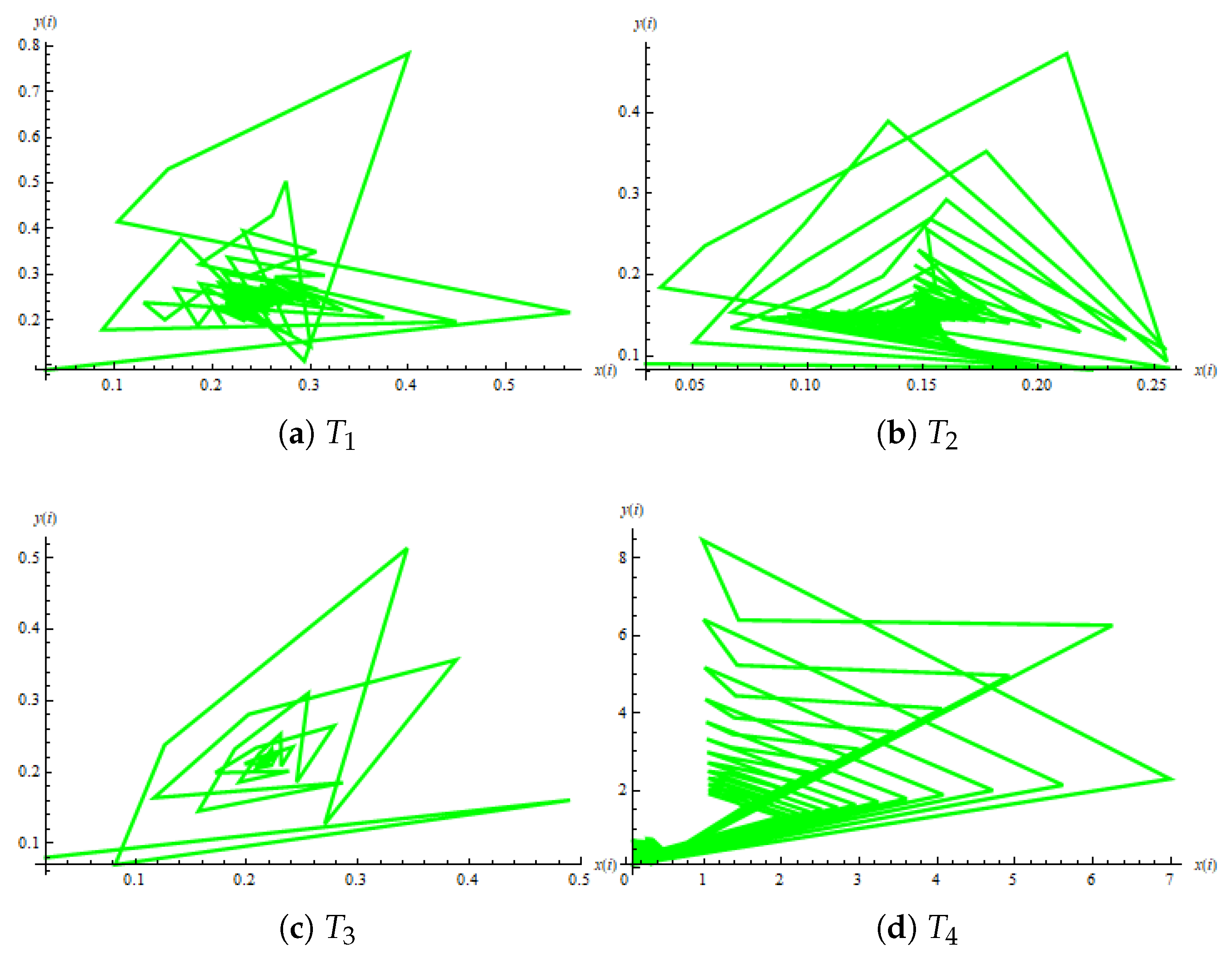
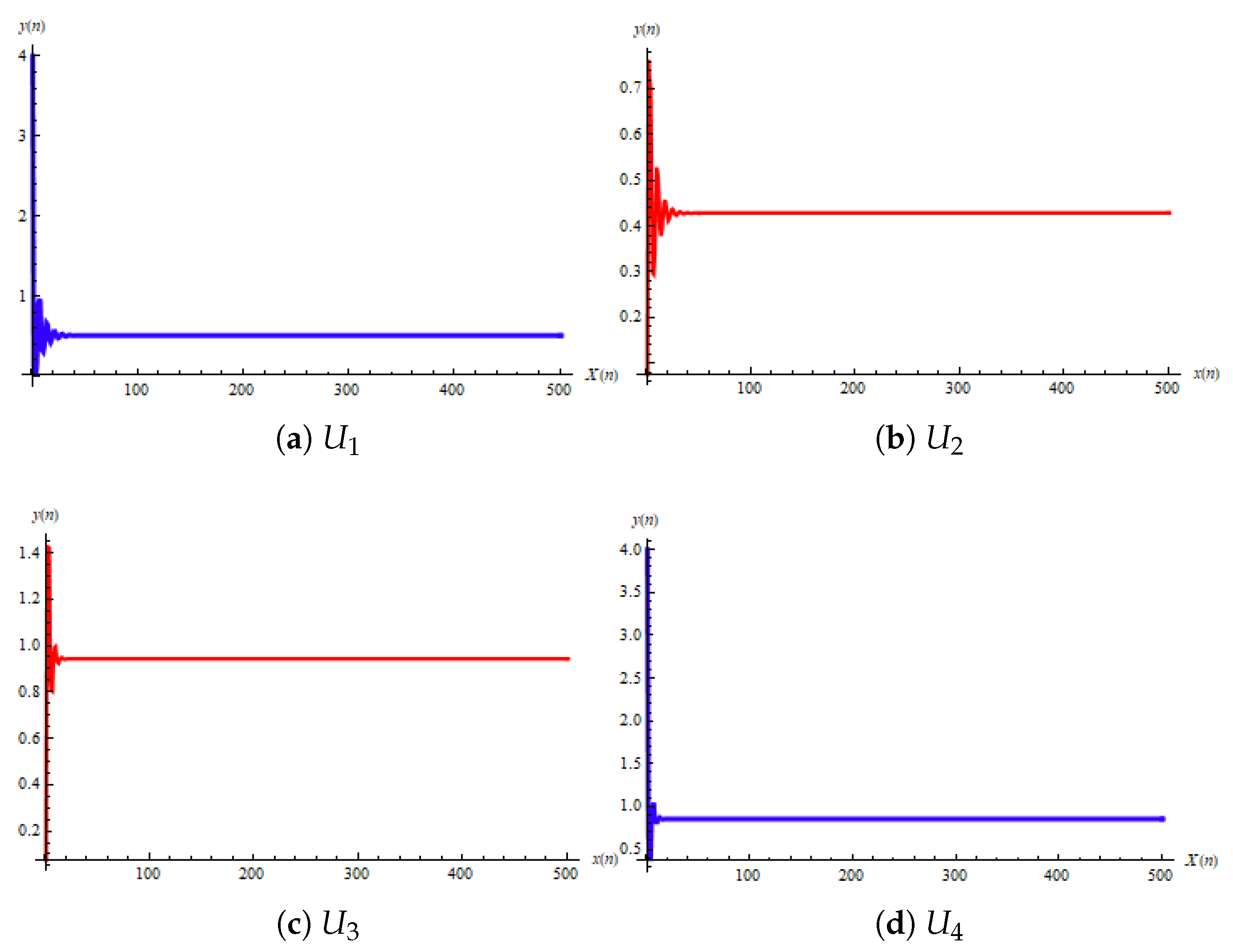
We take different values for the parameters D, E, and F (

Table 1. Parameters for (99) and its equilibrium point.

Parameters (D, E, F)	Equilibrium Point	Trajectory
$0.03$, $0.06$, $0.07$	$0.246282$	$T_1$
$0.01$, $0.02$, $0.03$	$0.15961$	$T_2$
$0.06$, $0.02$, $0.13$	$0.218377$	$T_3$
$0.75$, $0.02$, $0.03$	$1.59206$	$T_4$

and

Table 2. Parameters for (99) and its equilibrium point.

Parameters (D, E, F)	Equilibrium Point	Trajectory
$0.2$, $0.5$, $0.8$	$0.4281$	$U_1$
$0.3$, $0.7$, $0.9$	$0.5105$	$U_2$
12, 15, 18	$0.9421$	$U_3$
20, $0.25$, 35	$0.8544$	$U_4$

) and the initial values $t_{-3}$, $t_{-2}$, $t_{-1}$, and $t_0$ to graphically verify the results. The obtained plots are presented in Figure 3 and Figure 4.

5. Conclusions

Engineering, ecology, the social sciences, and various other disciplines extensively utilize mathematical modeling to address real-world challenges. When these challenges exhibit continuous behavior, they are typically modeled using differential equations, whereas discrete systems are represented through difference equations. In recent years, difference equations have gained prominence in discrete system modeling. Since uncertainty and imprecision naturally arise in practical applications, fuzzy theory serves as a valuable tool in extending the framework of difference equations.

The study of fuzzy difference equations (FDEs) has led to numerous significant findings, and ongoing research continues to expand this field. In this article, we investigated a non-homogeneous fourth-order exponential FDE with fuzzy initial conditions, external forcing functions, and fuzzy coefficients. Furthermore, we analyzed the equilibrium point and stability properties of a system described by an FDE. Numerical simulations were provided to validate the theoretical analysis. Our findings contribute to the understanding of FDE-based mathematical models in population dynamics and economic systems.

This research encountered several challenges:

• Managing the computational complexity of higher-order equations involving exponential terms and fuzzy parameters.
• Designing efficient numerical methods to verify theoretical results, especially for large initial conditions.

Unlike previous studies that primarily examined second- and third-order rational fuzzy difference equations, this research highlights the effectiveness of exponential models in capturing more complex dynamics. Our results on boundedness and global stability extend earlier works, which mainly focused on local stability or asymptotic behavior in simpler settings.

The implications of these results extend to artificial intelligence, where fuzzy difference equations can be employed to model adaptive learning systems. Additionally, biological models with exponential growth or decay patterns, such as population dynamics under uncertainty, can benefit from this approach. Similarly, control systems and economic models can integrate this framework to manage uncertainty more effectively.

Future research may explore fuzzy population dynamics in greater depth. Moreover, further qualitative properties, such as invariant intervals and bifurcation analysis, can be investigated within this modeling framework.

References

1. Dubois, D.; Prade, H. Possibility Theory: An Approach to Computerized Processing of Uncertainty; Plenum Publishing Corporation: New York, NY, USA, 1988. [Google Scholar]
2. Din, Q. Global stability of a population model. Chaos Solitons Fractals 2014, 59, 119–128. [Google Scholar] [CrossRef]
3. Din, Q.; Khan, K.; Nosheen, A. Stability Analysis of a System of Exponential Difference Equations. Discret. Dyn. Nat. Soc. 2014, 2014, 375890. [Google Scholar] [CrossRef]
4. Din, Q. Asymptotic Behavior of a Second-Order Fuzzy Rational Difference Equation. J. Discret. Math. 2015, 2015, 524931. [Google Scholar] [CrossRef]
5. Kalabušić, S.; Kulenović, M.; Pilav, E. Dynamics of a two-dimensional system of rational difference equations of Leslie–Gower type. Adv. Differ. Equ. 2011, 2011, 29. [Google Scholar] [CrossRef]
6. Deeba, E.; de Korvin, A.; Koh, E. A fuzzy difference equation with an application. J. Differ. Equ. Appl. 1996, 2, 365–374. [Google Scholar] [CrossRef]
7. Deeba, E.; de Korvin, A. Analysis by fuzzy difference equations of a model of CO2 level in the blood. Appl. Math. Lett. 1999, 12, 33–40. [Google Scholar] [CrossRef]
8. Mondal, S.; Vishwakarma, D.; Saha, A. Solution of Second Order Linear Fuzzy Difference Equation by Lagrange’s Multiplier Method. J. Soft Comput. Appl. 2016, 2016, 11–27. [Google Scholar] [CrossRef]
9. Khastan, A. Fuzzy Logistic Difference Equation. Iran. J. Fuzzy Syst. 2018, 15, 55–66. [Google Scholar] [CrossRef]
10. Papaschinopoulos, G.; Papadopoulos, B. On the fuzzy difference equation xn+1 = A + B/xn. Soft Comput. 2002, 6, 456–461. [Google Scholar] [CrossRef]
11. Papaschinopoulos, G.; Papadopoulos, B. On the fuzzy difference equation xn+1 = a + xn/xnm. Fuzzy Sets Syst. 2002, 129, 73–81. [Google Scholar] [CrossRef]
12. Memarbashi, R.; Ghasemabadi, A. Fuzzy difference equations of Volterra type. Int. J. Nonlinear Anal. Appl. 2013, 4, 74–78. [Google Scholar] [CrossRef]
13. Stefanidou, G.; Papaschinopoulos, G.; Schinas, C. On an Exponential-Type Fuzzy Difference Equation. Adv. Differ. Equ. 2010, 2010, 196920. [Google Scholar] [CrossRef]
14. Sun, T.; Su, G.; Qin, B. On the fuzzy difference equation xn = F(xn−1, xnk). Fuzzy Sets Syst. 2020, 387, 81–88. [Google Scholar] [CrossRef]
15. Wang, C.; Su, X.; Liu, P.; Hu, X.; Li, R. On the dynamics of a five-order fuzzy difference equation. J. Nonlinear Sci. Appl. 2017, 10, 3303–3319. [Google Scholar] [CrossRef]
16. Zhang, Q.; Liu, J.; Luo, Z. Dynamical behavior of a third-order rational fuzzy difference equation. Adv. Differ. Equ. 2015, 2015, 108. [Google Scholar] [CrossRef]
17. Zhang, Q.; Yang, L.; Liao, D. Behavior of Solutions to a Fuzzy Nonlinear Difference Equation. Iran. J. Fuzzy Syst. 2012, 9, 1–12. [Google Scholar] [CrossRef]
18. Zhang, Q.; Yang, L.; Liao, D. On first order fuzzy Ricatti difference equation. Inf. Sci. 2014, 270, 226–236. [Google Scholar] [CrossRef]
19. Stefanini, L. A generalization of Hukuhara difference and division for interval and fuzzy arithmetic. Fuzzy Sets Syst. 2010, 161, 1564–1584. [Google Scholar] [CrossRef]
20. Khastan, A.; Alijani, Z. On the New Solutions to the Fuzzy Difference Equation xn+1 = A + B/xn. Fuzzy Sets Syst. 2019, 358, 64–83. [Google Scholar] [CrossRef]
21. Khastan, A. New solutions for first order linear fuzzy difference equations. J. Comput. Appl. Math. 2017, 312, 156–166. [Google Scholar] [CrossRef]
22. Zhang, Q.; Lin, F.; Zhong, X. On discrete time Beverton–Holt population model with fuzzy environment. Math. Biosci. Eng. 2019, 16, 1471–1488. [Google Scholar] [CrossRef] [PubMed]
23. Papaschinopoulos, G.; Stefanidou, G. Boundedness and asymptotic behavior of the solutions of a fuzzy difference equation. Fuzzy Sets Syst. 2003, 140, 523–539. [Google Scholar] [CrossRef]
24. Yalçınkaya, İ.; Tollu, D.T.; Khastan, A.; Ahmad, H.; Botmart, T. Qualitative behavior of a higher-order fuzzy difference equation. AIMS Math. 2023, 8, 6309–6322. [Google Scholar] [CrossRef]
25. Han, C.; Li, L.; Su, G.; Sun, T. Dynamical behaviors of a k-order fuzzy difference equation. Open Math. 2022, 20, 391–403. [Google Scholar] [CrossRef]
26. Zhang, Q.; Zhang, W.; Lin, F.; Li, D. On dynamic behavior of second-order exponential-type fuzzy difference equation. Fuzzy Sets Syst. 2021, 419, 169–187. [Google Scholar] [CrossRef]
27. Atpinar, S.; Yazlik, Y. Qualitative behavior of exponential type of fuzzy difference equations system. J. Appl. Math. Comput 2023, 69, 4135–4162. [Google Scholar] [CrossRef]
28. Bede, B. Mathematics of Fuzzy Sets and Fuzzy Logic; Springer: Berlin/Heidelberg, Germany, 2013. [Google Scholar] [CrossRef]
29. Alamin, A.; Mondal, S.; Alam, S.; Goswami, A. Solution and stability analysis of non-homogeneous difference equation followed by real life application in fuzzy environment. Sadhana 2020, 45, 185. [Google Scholar] [CrossRef]
30. Kocic, V.; Ladas, G. Global Behavior of Nonlinear Difference Equations of Higher Order with Applications; Springer Science+Business Media: Dordrecht, The Netherlands, 1993. [Google Scholar] [CrossRef]
Figure 1. Evolution of the solution of Equation (63) for different values of σ . The three subfigures illustrate the behavior of the solution at σ = 0.0 (a), σ = 0.5 (b), and σ = 1.0 (c). The asterisk (∗) and line indicate the trend of convergence towards the equilibrium point t ¯ .
Axioms 14 00118 g001
Figure 2. Solution trajectories of the fuzzy difference equation (98) under varying initial conditions. The subfigures demonstrate the impact of different parameter choices on the system’s evolution. The asterisk (∗) and line highlight critical points and trends in the solution space.
Axioms 14 00118 g002
Figure 3. Trajectories obtained for parameters given in Table 1.
Axioms 14 00118 g003
Figure 4. Trajectories obtained for parameters given in Table 2.
Axioms 14 00118 g004