Effects of Predation-Induced Emigration on a Landscape Ecological Model

Abstract

Predators impact prey populations directly through consumption and indirectly via trait-mediated effects like predator-induced emigration (PIE), where prey alter movement due to predation risk. While PIE can significantly influence prey dynamics, its combined effect with direct predation in fragmented habitats is underexplored. Habitat fragmentation reduces viable habitats and isolates populations, necessitating an understanding of these interactions for conservation. In this paper, we present a reaction–diffusion model to investigate prey persistence under both direct predation and PIE in fragmented landscapes. The model considers prey growing logistically within a bounded habitat patch surrounded by a hostile matrix. Prey move via unbiased random walks internally but exhibit biased movement at habitat boundaries influenced by predation risk. Predators are assumed constant, operating on a different timescale. We examine three predation functional responses—constant yield, Holling Type I, and Holling Type III—and three emigration patterns: density-independent, positive density-dependent, and negative density-dependent emigration. Using the method of sub- and supersolutions, we establish conditions for the existence and multiplicity of positive steady-state solutions. Numerical simulations in one-dimensional habitats further elucidate the structure of these solutions. Our findings demonstrate that the interplay between direct predation and PIE crucially affects prey persistence in fragmented habitats. Depending on the functional response and emigration pattern, PIE can either mitigate or amplify the impact of direct predation. This underscores the importance of incorporating both direct and indirect predation effects in ecological models to better predict species dynamics and inform conservation strategies in fragmented landscapes.

1. Introduction

Studies have shown that predators have both direct (density-mediated) and indirect (trait-mediated indirect) effects on prey populations (see [1,2,3,4]). In fact, it is widely accepted that ecological communities are replete with trait-mediated indirect effects arising from phenotypic plasticity, and these effects are important to community dynamics (see [1,3,5]). Trait-mediated behavioral responses to predators have the potential to greatly affect the dynamics of a population (see [1,3,4]). One such effect is trait-mediated emigration, wherein the prey changes its emigration patterns due to the presence of a predator [2,6,7,8]. This can, in turn, modify population dynamics and species interactions (see [9], for example). Few empirical studies have considered this effect in the predator–prey context, where increased predation risk was shown to increase the emigration rates of prey. For example, ref. [2] found evidence of predator-induced emigration (PIE) in a spider (predator) and planthopper (prey) system, and concluded that at high predator density, the predator had a greater impact on prey density through induced emigration than consumption (also see [6,7,8]).

Human-dominated habitat fragmentation continues at unprecedented levels, giving rise to the need for a better understanding of the consequences of density dependence and its role in conservation efforts [10,11,12,13,14]. Habitat fragmentation reduces viable habitat or patch size and also separates populations among much smaller residual patches which are surrounded by a human-modified “matrix” with varying degrees of hostility [11]. The modeling of theoretical populations has seen great success in predicting patch- and even landscape-level patterns in response to habitat fragmentation. The reaction diffusion framework has been particularly successful at providing better understanding of the coupling of density dependent growth mechanisms with density dependent movement or dispersal (see [15]). The framework’s ability to handle space explicitly at the landscape level, including modeling animal movement behavior differences when a patch boundary is reached, has been well demonstrated [16,17,18,19].

The modeling of predator–prey population dynamics dates back to the classic works of [20,21]. A key component of those models is the predator functional response, the relationship between prey consumption per predator per unit of time as prey density increases [22,23]. In the original formulation of the Lotka–Volterra model, predators and prey were assumed to encounter each other at random, resulting in a constant rate of prey consumption as the prey density increased. Subsequent derivations of the functional response have included more realistic predator behaviors such as handling time constraints and predator satiation that result in a decreasing rate of prey consumption as the prey density increases (Holling’s type II functional response), or learning or switching to more abundant or profitable prey that results in an increasing, then decreasing, rate of prey consumption as the prey density increases (Holling’s type III functional response) (see [22,24,25]). Over the years, many studies have expanded on Holling’s seminal work and investigated the biological implications of a wide range of predator functional responses (e.g., see [26,27,28,29,30]).

In this paper, we employ a model based on the reaction diffusion framework to study the persistence of a prey species that is experiencing both direct (density-mediated) and indirect (predator-induced emigration) effects while facing habitat fragmentation. This framework was derived in [19] (but also see [31]) and connects assumptions regarding movement behavior at the individual level to the patch- and landscape levels. To our knowledge, no other study has examined the linkage between predator presence, the prey’s density–emigration relationship and prey population dynamics in a landscape context. Here, we envision a prey species which inhabits a patch $\Omega$ which is a bounded domain in ${\mathbb{R}}^N$; $N>1$ with smooth boundary $\partial \Omega$ or $\Omega =(0,1)$ that is surrounded by a hostile matrix. In the framework, prey grow logistically and move according to an unbiased random walk inside the patch and in the matrix but follow a biased random walk at the patch/matrix interface, making an emigration decision based upon the presence of a predator. We assume that the predator is acting on a different timescale than the prey and thus assume a constant predator population. The nondimensionalized steady-state equation for the model is then given by

$$\left\{\begin{array}{c}-\Delta u=\lambda \left[u(1-u)-h(c,u)\right];\Omega \\ {\displaystyle \frac{\partial u}{\partial \eta }}+\sqrt{\lambda }\gamma g(c,u)u=0;\partial \Omega \end{array}\right.$$

(1)

where $u\left(x\right)$ is the prey population density for $x\in \Omega$, $\lambda >0$ is a composite parameter that is proportional to the patch size squared, $\gamma >0$ is a parameter that quantifies the matrix hostility, and ${\displaystyle \frac{\partial u}{\partial \eta }}$ is the outward normal derivative of u. Here, $g(c,s)={\displaystyle \frac{1-\alpha \left(s\right)}{\alpha \left(s\right)}}$, where $\alpha \left(s\right)$ is the probability of the organism staying inside $\Omega$ upon reaching the boundary and represents emigration patterns such as density-independent emigration (DIE) when $\alpha$ is a constant, positive density-dependent emigration (+DDE) when $1-\alpha \left(s\right)$ is increasing, and negative density-dependent emigration (−DDE) where $1-\alpha \left(s\right)$ is decreasing.

• Here, $h(c,s)$ represents the predation functional response, and we consider the following forms:

(i)

Constant-yield predation (CYP): $h_1(c,s)=c; c>0$.

(ii)

Constant-effort predation: Holling Type I functional response: $h_2(c,s)=cs; c>0$.

(iii)

Prey switching predation: Holling Type III functional response: $h_3(c,s)={\displaystyle \frac{c{s}^2}{m+s^2}}$; $c>0, m>0$.

For the emigration form g, we consider the following:

(i)

Density-independent emigration (DIE): $g_1(c,s)=1+\mu c; \mu \ge 0$

(ii)

Positive density-dependent emigration (+DDE): $g_2(c,s)=1+\beta s+\mu c; \mu \ge 0, \beta >0$

(iii)

Negative density-dependent emigration (−DDE): $g_3(c,s)={\displaystyle \frac{1}{1+\beta s}}+\mu c; \mu \ge 0, \beta >0$

Where $\mu \ge 0$ is a composite parameter that measures the prey’s sensitivity to the presence of the predator (we will also denote this as the strength of the PIE relationship) and $\beta \ge 0$ is a composite parameter that dictates the strength of the DDE form (see [32]). For example, a −DDE form with $\beta \approx 0$ is very similar to DIE, while one with $\beta \gg 1$ shows a strong negative relationship between density and emigration.

Recently, several studies have either considered models similar to (1) but with only direct effects of predation or indirect effects such as PIE (see [29,33,34,35,36,37,38]).

To date, few, if any, studies have considered the combined effects of both the direct and indirect effects of the predation of a prey in the presence of habitat fragmentation. Our motivation here is to compare the structure of the positive solutions for (1) when predation does not affect the emigration rate ($\mu =0$) to the case when predation does influence the emigration rate ($\mu >0$). We establish several existence, non-existence, and multiplicity results via the method of sub- and supersolutions and then numerically explore the structure of positive steady-state solutions in the one-dimensional case where more complete results and biological interpretation can be obtained.

To present our main results, we first describe a useful eigenvalue problem. Given $M,b>0$ and $\gamma >0$, let $E_1(M,b,\gamma )$ be the principal eigenvalue of

$$\left\{\begin{array}{c}-\Delta \varphi =EM\varphi ;\Omega \\ {\displaystyle \frac{\partial \varphi }{\partial \eta }}+\gamma b\sqrt{E}\varphi =0;\partial \Omega \end{array}\right.$$

(2)

with corresponding eigenfunction $\varphi >0;\overline{\Omega }$. Further, let $g_0(\mu ,c)=g_i(c,0)=1+\mu c$ for $i=1,2,3$, and $z_0\left(c\right)$ be the positive falling zero of $f(c,s)=s(1-s)-h(c,s)$. Throughout this paper, to ensure the existence of positive solutions for (1), we assume that $c>0$ is a fixed number small enough so that this $z_0$ exists and $F(c,z_0)>0$, where $F(c,s)={\int }_0^{s}f(c,r)dr$. Now, we state our main results.

• Results for Case A: Constant-Yield Predation$h(c,s)=h_1(c,s)\equiv c$

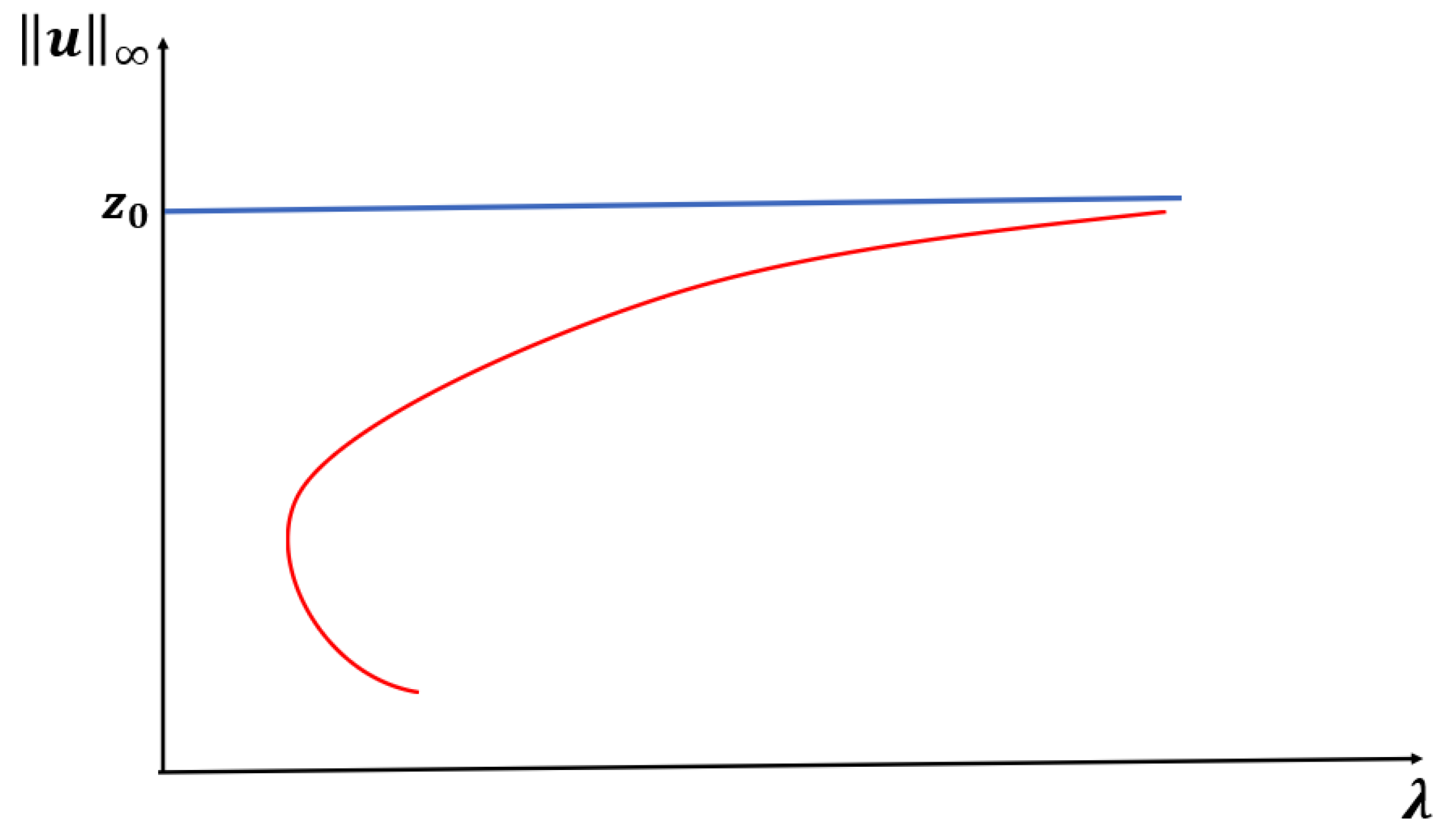
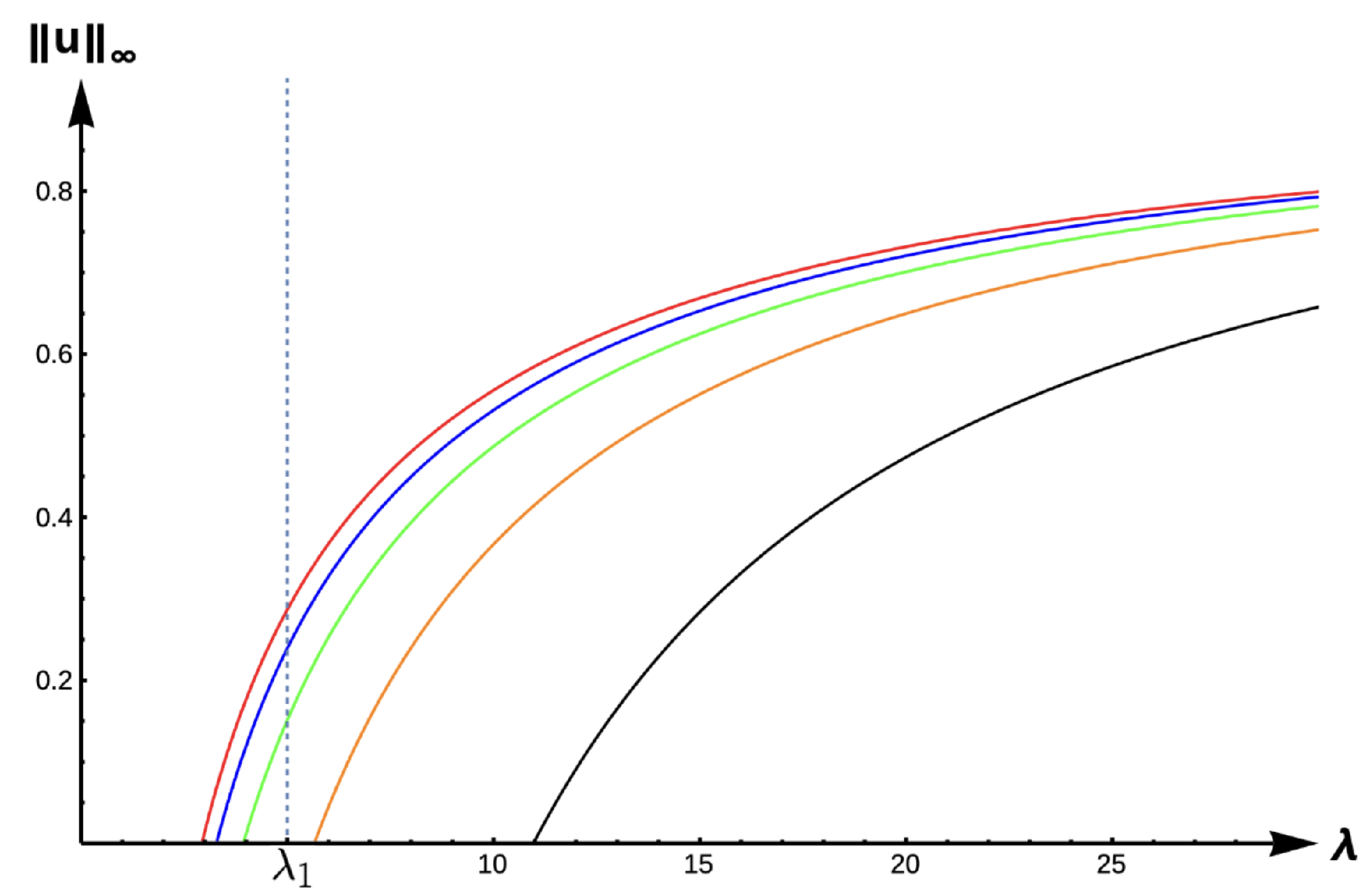
Notice that for $c<{\displaystyle \frac{1}{4}}$, $f(c,s)$ has two distinct zeros, $z_0,z_1$ with $0<z_1<z_0$. We now state the results for this case with an expected bifurcation curve presented in Figure 1.

Figure 1. An expected bifurcation diagram for Case A constant-yield predation.

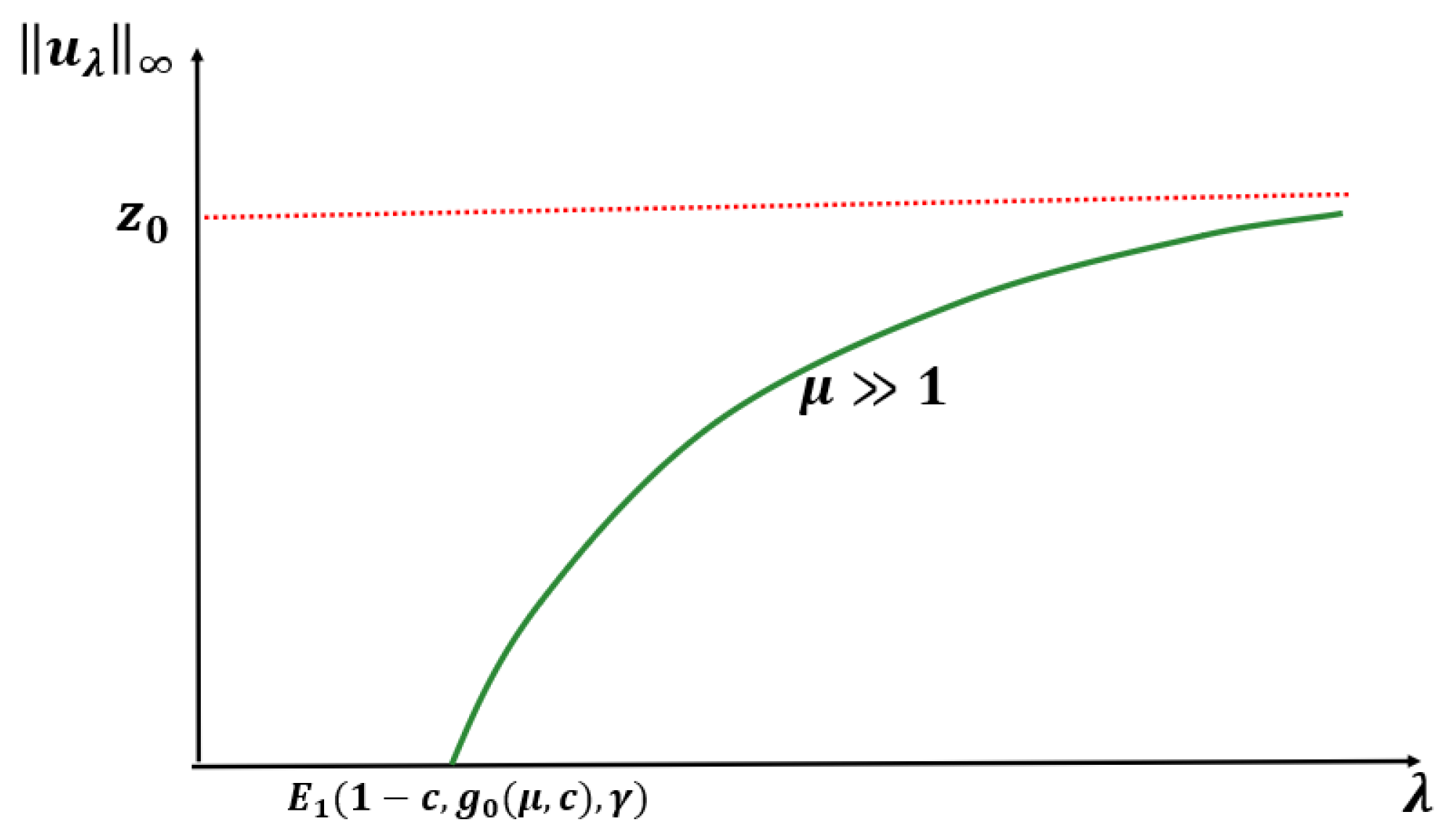
Theorem 1.

Let $g=g_1,g_2,$ or $g_3$ and $\mu \ge 0$ be fixed. Then, (1) has at least one positive solution $u_{\lambda }$ for $\lambda \gg 1$ such that $\parallel u_{\lambda }{\parallel }_{\infty }⟶z_0$ as $\lambda ⟶\infty$ (see Figure 1). Moreover, the time-dependent model predicts extinction for any $\lambda >0$ when the initial density profile is below $z_1$.

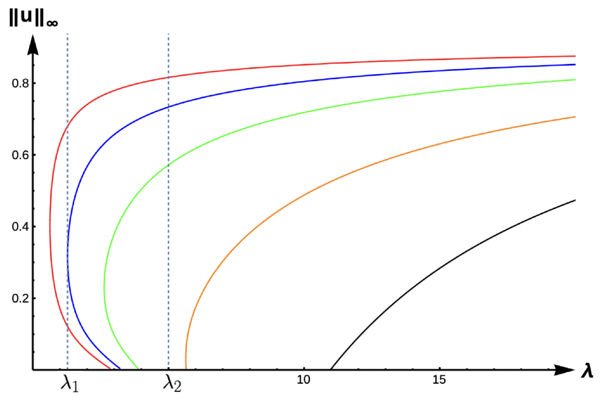
For the next two cases ($h=h_2$ and $h=h_3$), we also focus on exploring the existence of a patch-level Allee effect (PAE). In this scenario, the trivial solution and at least one other positive solution of (1) are both stable, giving rise to a population density threshold that must be maintained to ensure the persistence of the population. A sufficient condition for a PAE is the existence of a range of $\lambda$ to the left of $E_1(M,g_0(\mu ,c),\gamma )$ where at least one positive solution exists (see Figure 2 and [32]). Here, $M=1-c$ when $h=h_2$ and $M=1$ when $h=h_3$. Furthermore, when $h=h_1$, numerical evidence shows that there is also a range of $\lambda$ with multiple positive solutions. However, this is a well-known open problem to establish analytically (see the literature on semi-positone problems).

Figure 2. Bifurcation diagram exhibiting a patch level Allee effect.

• Results for Case B: Constant-Effort Predation:$h(c,s)=h_2(c,s)=cs$
• In this case, the roots of $f(c,s)$ are zero and $z_0$. We now state the results for this case.

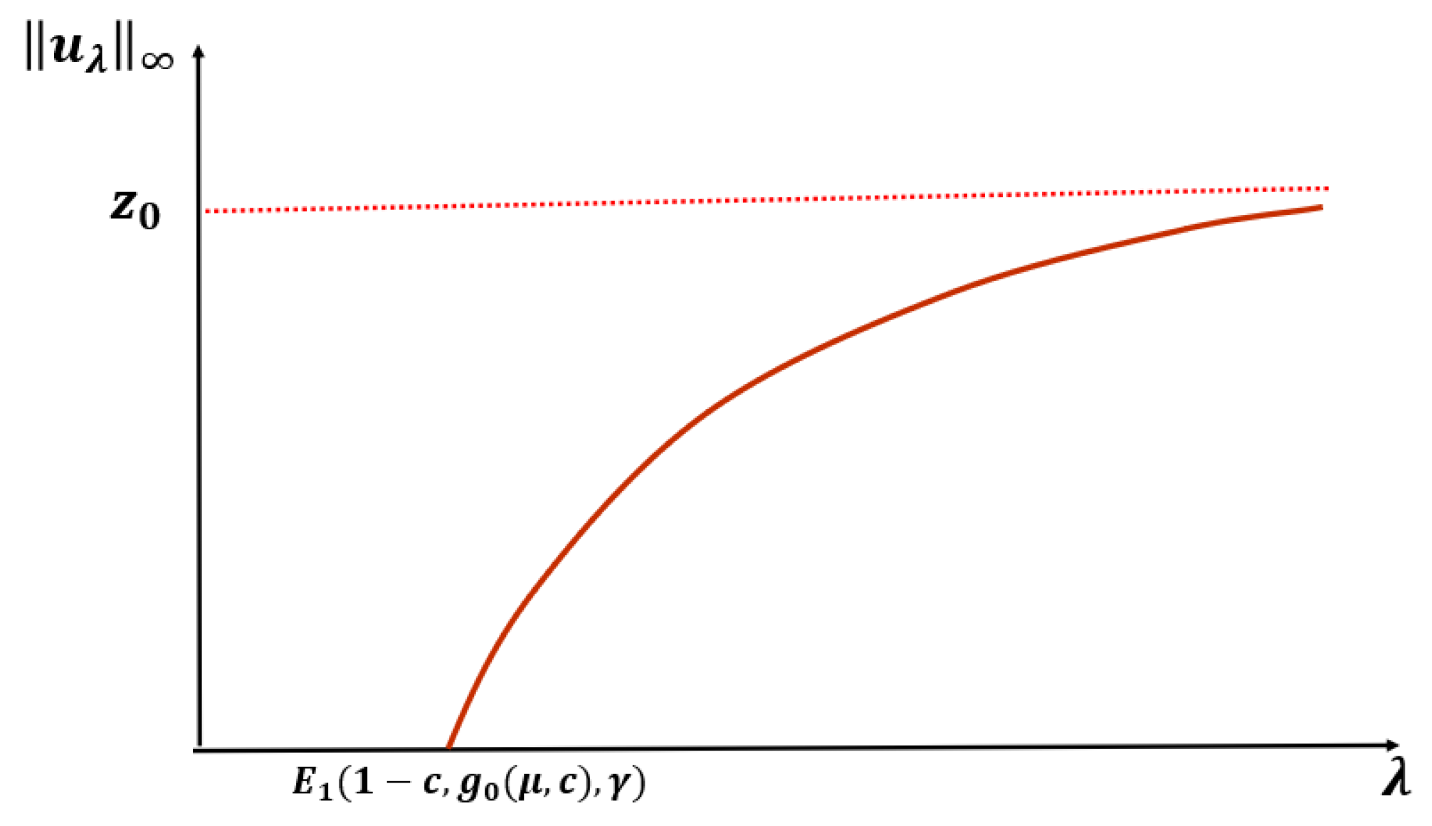
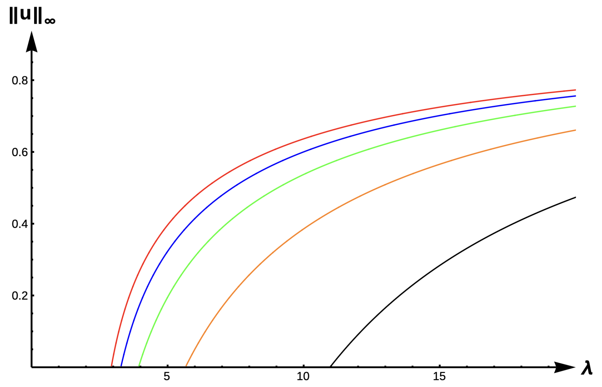
Theorem 2.

Let $g=g_1$ or $g_2$ and $\mu \ge 0$ be fixed. Then, (1) has a unique positive solution $u_{\lambda }$ for $\lambda >E_1(1-c,g_0(\mu ,c),\gamma )$ and no positive solution for $\lambda <E_1(1-c,g_0(\mu ,c),\gamma )$. Further, $\parallel u_{\lambda }{\parallel }_{\infty }\to 0$ as $\lambda \to E_1(1-c,g_0(\mu ,c),\gamma )$ and $\parallel u_{\lambda }{\parallel }_{\infty }\to z_0$ as $\lambda \to \infty$ (see Figure 3).

Figure 3. An expected bifurcation diagram for Case B constant-effort predation with $g=g_1$ (DIE) or $g=g_2$ (+DDE).

Remark 1.

Let $g=g_1$ or $g_2$, ${\mu }_1>{\mu }_2\ge 0$, $\lambda >E_1(1-c,g_0({\mu }_1,c),\gamma )$, $u_{{\mu }_1}$ and $u_{{\mu }_2}$ be the unique positive solutions of (1) when $\mu ={\mu }_1$ and $\mu ={\mu }_2$, respectively, then $u_{{\mu }_1}\left(x\right)<u_{{\mu }_2}\left(x\right),\forall x\in \overline{\Omega }$ (see Figure 4).

Figure 4. Variation of bifurcation diagrams when $\mu$ varies for Case B constant-effort predation, where $0<{\mu }_2<{\mu }_1<\infty$.

Before we state our next theorem, we define

$$\left\{\begin{array}{c}{\lambda }^{*}={\displaystyle \frac{E_1\left(1-c,g_0(\mu ,c),\gamma \right)+E_1\left(1-c,\frac{g_0(\mu ,c)+\mu c}{2},\gamma \right)}{2}}\\ I:=\left[{\lambda }^{*},E_1(1-c,g_0(\mu ,c),\gamma )\right]\end{array}\right.$$

(3)

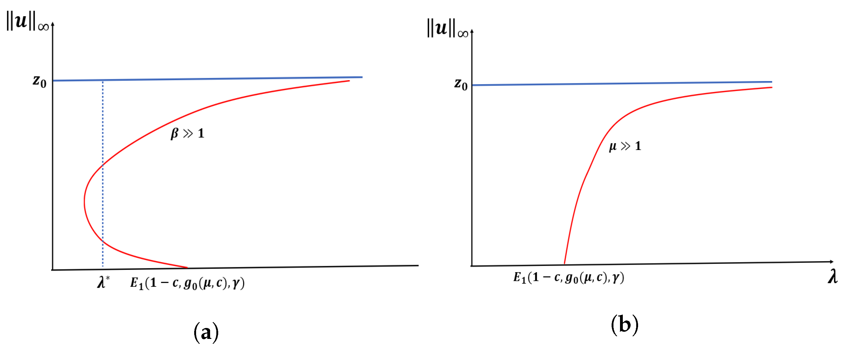
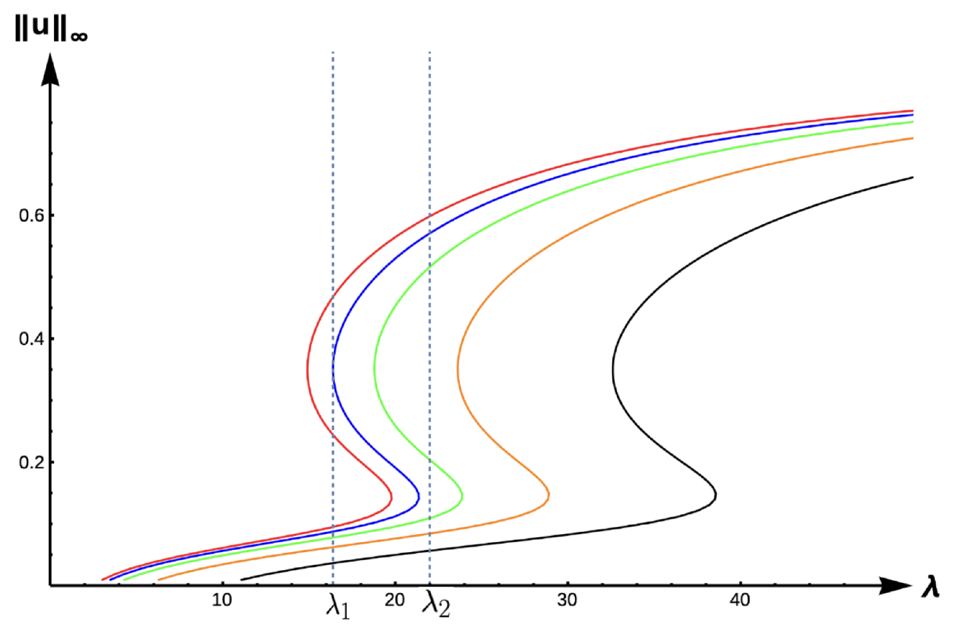
Theorem 3.

Let $g=g_3$. Then, for fixed $c>0$ and $\mu \ge 0$, there exists ${\beta }_1\left(\mu \right)>0$ such that a PAE occurs for $\lambda \in I$ for $\beta >{\beta }_1\left(\mu \right)$. Further, if ${\lambda }_0<E_1^D$ and $\beta >0$ are fixed, then there exists ${\mu }_1(\beta ,{\lambda }_0)>0$ such that (1) has no positive solution for $\lambda <{\lambda }_0$ when $\mu >{\mu }_1(\beta ,{\lambda }_0)$, where $E_1^D$ is the principal eigenvalue of

$$\left\{\begin{array}{c}-\Delta \varphi =E\varphi ;\Omega \\ \varphi =0;\partial \Omega \end{array}\right.$$

(4)

(see Figure 5).

Figure 5. Expected bifurcation diagrams for Case B constant-effort predation when $g=g_3$ (−DDE) with $\beta \gg 1$ in (a) and $\mu \gg 1$ in (b).

Next, we state the following conjecture based on our numerical results (see Section 2).

Conjecture: For any $g_i$ and fixed $\beta >0$, when $\mu \gg 1$, (1) has no positive solution for $\lambda <E_1(1-c,g_0(\mu ,c),\gamma )$, and (1) has a unique positive solution $u_{\lambda }$ for $\lambda >E_1(1-c,g_0(\mu ,c),\gamma )$ such that $\parallel u_{\lambda }{\parallel }_{\infty }\to 0^{+}$ as $\lambda \to E_1{(1-c,g_0(\mu ,c),\gamma )}^{+}$ and $\parallel u_{\lambda }{\parallel }_{\infty }\to z_0$ as $\lambda \to \infty$ (see Figure 6).

Figure 6. Expected bifurcation diagram for Case B constant-effort predation for any DDE and when $\mu \gg 1$.

• Results for Case C: Prey Switching Predation: $h(c,s)=h_3(c,s)={\displaystyle \frac{c{s}^2}{m+s^2}}$

Here, we state two hypotheses before we state our results. Let $R>0$ be the radius of the largest ball that can be inscribed inside the domain $\Omega$, $C_N:={\displaystyle \frac{{(N+1)}^{N+1}}{2N^N}}$$(>1)$, $f^{*}(c,s):=\underset{r\in [0,s]}{max}f(c,r)$, and given a $b>0$, denote $v(\mu ,b,c)$ as the unique solution of

$$\left\{\begin{array}{c}-\Delta v=1;\Omega \\ {\displaystyle \frac{\partial v}{\partial \eta }}+\gamma \tau (b,c)g_{\infty }\left(c\right)v=0;\partial \Omega \end{array}\right.$$

(5)

with $\tau (b,c)=\sqrt{{\displaystyle \frac{2bN{C}_N}{R^{2}f(c,b)}}}$ and $g_{\infty }\left(c\right)=\underset{s\in [0,z_0\left(c\right)]}{min}g(c,s)$.

Now, we state two hypotheses regarding f:

(H₁):

there exist $a,b>0$ such that $a<b<{\displaystyle \frac{z_0}{C_N}}$ and ${\displaystyle \frac{a}{f^{*}(c,a)}}/{\displaystyle \frac{b}{f(c,b)}}>{\displaystyle \frac{2N{C}_N{\parallel v(\mu ,b,c)\parallel }_{\infty }}{R^2}}$.

(H₂):

there exist $r_1\in (0,b)$ and $r_2\in (b{C}_N,z_0)$ such that f is non-decreasing in $(r_1,r_2)$.

Define

$$\left\{\begin{array}{c}{\lambda }^{**}={\displaystyle \frac{E_1\left(1,g_0(\mu ,c),\gamma \right)+E_1\left(1,\frac{g_0(\mu ,c)+\mu c}{2},\gamma \right)}{2}}\\ I^{*}:=\left[{\lambda }^{**},E_1(1,g_0(\mu ,c),\gamma )\right].\end{array}\right.$$

(6)

Theorem 4.

Let $g=g_3$. Then, for $c>0$ and fixed $\mu >0$, there exists ${\beta }_1\left(\mu \right)>0$ such that a PAE occurs for $\lambda \in I^{*}$ for $\beta >{\beta }_1\left(\mu \right)$. Further, if ${\lambda }_0<E_1^D$ and $\beta >0$ are fixed, there exists ${\mu }_1(\beta ,{\lambda }_0)>0$ such that (1) has no positive solution for $\lambda <{\lambda }_0$ when $\mu >{\mu }_1(\beta ,{\lambda }_0)$.

Theorem 5.

Let $g=g_1$, $g=g_2$, or $g=g_3$ with β be fixed. Let $\left(H_1\right)$ and $\left(H_2\right)$ hold. Then (1) has at least three positive solutions for $\lambda \in \left(max\left\{E_1(1,g_0(\mu ,c),\gamma ),{\displaystyle \frac{2bN{C}_N}{R^{2}f(c,b)}}\right\},min\left\{{\displaystyle \frac{a}{{\parallel v(\mu ,b,c)\parallel }_{\infty }{f}^{*}(c,a)}},{\displaystyle \frac{2r_{2}N}{f(c,b)R^2}}\right\}\right)$ (see Figure 7).

Figure 7. Occurrence of an S-shaped bifurcation diagram for Case C prey switching predation for any DDE form.

Remark 2.

In Section 4, when Ω is a ball of radius R, we prove that f and g satisfy the hypothesis of Theorem 5 for certain parameter values when μ is large.

Theorem 6.

Let $g=g_1$ or $g=g_2$. Then, (1) has no positive solution for $\lambda <E_1(1,g_0(\mu ,c),\gamma )$ (see Figure 7).

Remark 3.

In Case A, (1) has no positive solutions for $\lambda \approx 0$ and one can easily adapt the techniques used in the literature of semi-positone problems with Dirichlet boundary conditions to prove this. For Cases B and C, we will later establish that (1) has no positive solutions for $\lambda <E_1(1,g_{\infty }\left(c\right),\gamma )$.

In Section 2, we numerically compute complete bifurcation diagrams of the positive solutions in the one-dimensional case where $\Omega =(0,1)$ and discuss their biological relevance. We provide some mathematical preliminaries in Section 3, and in Section 4 we construct several sub- and supersolutions that we will use to establish our analytical results. Finally, we prove Theorems 1–6 and Remark 1 in Section 5.

2. One-Dimensional Results and Biological Conclusions

In this section, we present computationally generated results for the one-dimensional case when $\Omega =(0,1)$. In this way, we obtain more detailed bifurcation diagrams and provide some biological conclusions of these results. Namely, we consider the steady-state model:

$$\left\{\begin{array}{c}-u^{″}=\lambda \left[u(1-u)-h(c,u)\right];(0,1)\\ -u^{\prime }\left(0\right)+\gamma \sqrt{\lambda }g(c,u\left(0\right))u\left(0\right)=0\\ u^{\prime }\left(1\right)+\gamma \sqrt{\lambda }g(c,u\left(1\right))u\left(1\right)=0\end{array}\right.$$

(7)

and study the structure of positive solutions via bifurcation curves ($\lambda$ vs. ${\parallel u\parallel }_{\infty }$ curves) in order to contrast model predictions of the cases: $\mu =0$ (when predation does not affect emigration probability) and $\mu >0$ (when predation does influence the emigration probability). Here, we denote ${\parallel u\parallel }_{\infty }$ as the maximum density of the positive solution of (7). We obtain complete bifurcation diagrams via a quadrature method (presented in Lemma 3 of Section 3 and numerical computation using Mathematica (Wolfram Research Inc., version 14.0). See [32,39], and [40] for extensions of the original quadrature method developed in [41] for the case of Dirichlet boundary conditions. For completeness, we prove the extension of the quadrature method employed here in Appendix A. For simplicity of presentation, we choose $c=0.1$ for $h_1$ and $h_2$, and $c=0.13$ and $m=0.01$ for $h_3$. We note that a full exposition of the parameter space is outside the scope of this current work. Rather, we choose certain parameter ranges to provide prototypical model predictions. We also highlight several cases where predator-induced emigration and the strength of this response as measured in $\mu$ plays a significant role on model predictions.

2.1. Results for Case A: Constant-Yield Predation $h(c,s)=c$

In this subsection, we present results for the constant-yield predation case, where we have fixed $c=0.1$ and $\gamma =1$.

We note that when $h(c,s)=h_1(c,s)=c$, our model has a semi-positone structure (see [29]), and for Lemma 3 to hold, the $\rho$-value must be between $\theta$ and $z_0$, where $\theta$ is the first positive zero of F and $z_0$ is the falling positive zero of f (see Figure 8).

Figure 8. Shapes of $f(c,s)$ and $F(c,s)$ in the constant-yield predation case: $h(c,s)=h_1(c,s)$.

Before we state our results, we denote the $\lambda$-value associated with the minimum patch size as ${\lambda }_{min}$, namely, ${\lambda }_{min}$ is proportional to the minimum size of the habitat that will allow unconditional population persistence.

2.1.1. Bifurcation Diagrams for DIE: $g(c,s)=g_1(c,s)=1+\mu c$

The evolution of bifurcation curves with respect to PIE strength $\mu$ is shown in Figure 9, while Table 1 shows the evolution of ${\lambda }_{min}$, the uniqueness region, and the multiplicity region. Notice that for all $\lambda >0$, the smaller root of $f(c,u)$ is a supersolution of (7), implying that the time-dependent problem would predict extinction for any size patch if the initial density distribution is too small. Here, $\mu =0$ corresponds to the case where predation does not influence the emigration probability. We observe that the bifurcation curves shift from left to the right, the multiplicity region increases, and the uniqueness region decreases as $\mu$ increases. The bifurcation curves are approaching the bifurcation curve corresponding to a case of a completely lethal matrix (Dirichlet boundary condition) as the PIE strength $\mu \to \infty$. For a given $\lambda$-value, we see that the number of positive steady states also varies as $\mu$ changes. To highlight changes in model predictions with respect to the PIE strength, consider a patch with fixed matrix hostility and patch size yielding a $\lambda ={\lambda }_1=17$ as shown in Figure 9. In the absence of PIE ($\mu =0$), there is a unique positive solution of (7), $\mu =1$ and $\mu =3$ show two positive solutions, and no positive solution is possible (extinction) when $\mu >{\mu }^{*}$ for some ${\mu }^{*}>3$. Notice also that the red curve ($\mu =0$) and the black curve ($\mu \to \infty$) define an envelope of possible bifurcation curves, where PIE would have an effect on the model predictions of the population’s persistence. In other words, only populations with patch sizes having corresponding $\lambda$-values lying in this envelope could be adversely affected by the presence of PIE.

Figure 9. Bifurcation diagram of positive solutions for (7) with $g_1(c,u)=1+\mu c$ (DIE). Note that the dashed line is for ${\lambda }_1=17$, red represents $\mu =0$, blue $\mu =1$, green $\mu =3$, orange $\mu =10$, and black $\mu \to \infty$.

Table 1. $g_1(c,u)=1+\mu c$.

$\mu$	0	1	3	5	10
${\lambda }_{min}$	11.83	12.85	14.64	16.12	18.86
Uniqueness Region	$(15.88,\infty )$	$(17.51,\infty )$	$(20.44,\infty )$	$(22.98,\infty )$	$(27.91,\infty )$
Multiplicity Region	$(11.83,15.88]$	$(12.85,17.51]$	$(14.64,20.44]$	$(16.12,22.98]$	$(18.86,27.91]$

2.1.2. Bifurcation Diagrams for +DDE $g(c,s)=g_2(c,s)=1+\beta u+\mu c$

In the case of +DDE with strength measured in the nondimensional parameter $\beta$, the bifurcation diagram given in Figure 10 is very similar to that of the DIE case (Figure 9), albeit shifted further to the right. The ${\lambda }_{min}$, uniqueness region, and multiplicity region are given in Table 2 for $\beta =1$, and in Table 3 for $\beta =10$ (a stronger +DDE response). Model predictions are identical for this case as the previous one, including our ability to identify $\lambda$-values where the number of positive solutions changes from one to two, and then to none, as $\mu$ increases in the respective envelope.

Figure 10. Bifurcation diagram of positive solutions for (7) with $g_2(c,u)=1+u+\mu c$ (+DDE with $\beta =1$). Note that red represents $\mu =0$, blue $\mu =1$, green $\mu =3$, orange $\mu =10$, and black $\mu \to \infty$.

Table 2. $g_2(c,u)=1+u+\mu c$ (with $\beta =1$).

$\mu$	0	1	3	5	10
${\lambda }_{min}$	13.46	14.27	15.70	16.92	19.28
Uniqueness Region	$(17.43,\infty )$	$(18.83,\infty )$	$(21.40,\infty )$	$(23.68,\infty )$	$(28.24,\infty )$
Multiplicity Region	$(13.46,17.43]$	$(14.27,18.83]$	$(15.70,21.40]$	$(16.92,23.68]$	$(19.28,28.24]$

Table 3. $g_2(c,u)=1+10u+\mu c$ (with $\beta =10$).

$\mu$	0	1	3	5	10
${\lambda }_{min}$	18.85	19.15	19.72	20.25	21.38
Uniqueness Region	$(24.02,\infty )$	$(24.73,\infty )$	$(26.11,\infty )$	$(27.41,\infty )$	$(30.33,\infty )$
Multiplicity Region	$(18.85,24.02]$	$(19.25,24.73]$	$(19.72,26.11]$	$(20.25,27.41]$	$(21.38,30.33]$

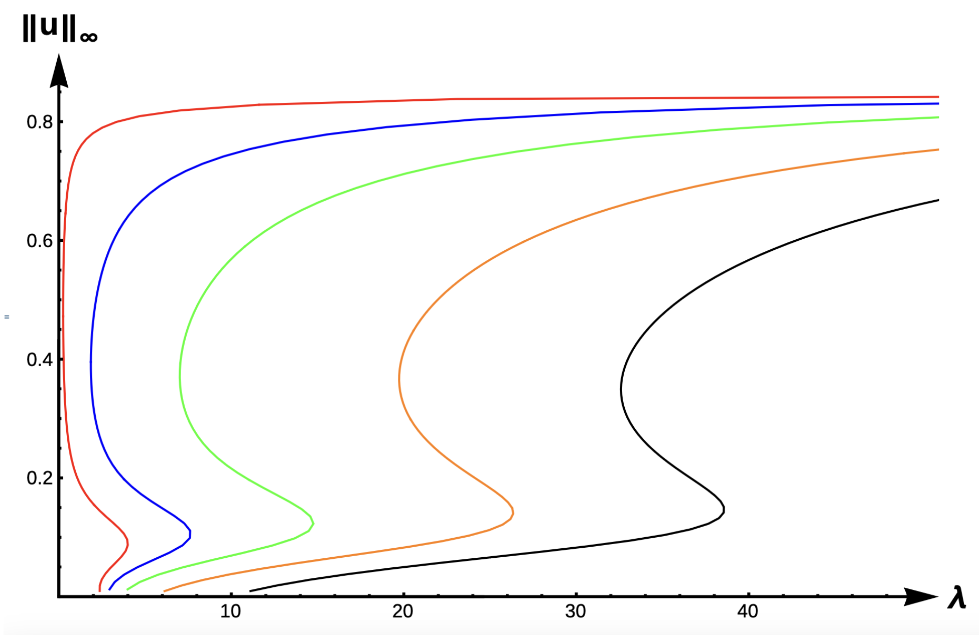
2.1.3. Bifurcation Diagrams for −DDE: $g(c,s)=g_3(c,s)={\displaystyle \frac{1}{1+\beta u}}+\mu c$

Figure 11 shows the evolution of bifurcation curves with respect to $\mu$, the −DDE case with $\beta =1$. Again, the bifurcation diagram is very similar to that of the DIE case (Figure 9), albeit shifted further to the left. The ${\lambda }_{min}$, uniqueness region, and multiplicity region are given in Table 4 for $\beta =1$, and in Table 5 for $\beta =10$ (a stronger +DDE response). Model predictions are identical for this case as the previous one, including our ability to identify $\lambda$-values where the number of positive solutions changes from one to two, and then to none, as $\mu$ increases in the respective envelope.

Figure 11. Bifurcation diagram of positive solutions for (7) with $g=g_3(c,u)={\displaystyle \frac{1}{1+u}}+\mu c$ (−DDE). Note that red represents $\mu =0$, blue $\mu =1$, green $\mu =3$, orange $\mu =10$, and black $\mu \to \infty$.

Table 4. $g_3(c,u)={\displaystyle \frac{1}{1+u}}+\mu c$ (with $\beta =1$).

$\mu$	0	1	3	5	10
${\lambda }_{min}$	9.72	11.07	13.36	15.19	18.40
Uniqueness Region	$(14.04,\infty )$	$(15.96,\infty )$	$(19.35,\infty )$	$(22.21,\infty )$	$(27.56,\infty )$
Multiplicity Region	$(9.72,14.04]$	$(11.07,15.96]$	$(13.36,19.35]$	$(15.19,22.21]$	$(18.40,27.56]$

Table 5. $g_3(c,u)={\displaystyle \frac{1}{1+10u}}+\mu c$ (with $\beta =10$).

$\mu$	0	1	3	5	10
${\lambda }_{min}$	1.21	2.72	6.23	9.54	15.42
Uniqueness Region	$(3.11,\infty )$	$(5.37,\infty )$	$(10.57,\infty )$	$(15.57,\infty )$	$(24.52,\infty )$
Multiplicity Region	$(1.21,3.11]$	$(2.72,5.37]$	$(6.23,10.57]$	$(9.54,15.57]$	$(15.42,24.52]$

2.2. Results for Case B: Constant-Effort Predation: $h(c,s)=h_2(c,s)=cs$

In this subsection, we present results for the constant-effort predation case, where we have fixed $c=0.1$ and $\gamma =1$. We note that $f(c,s)=s(1-s)-cs=s(1-c-s)$ has two zeros (0 and 0.9) when $c=0.1$. Here, Lemma 3 holds for $\rho \in (0,0.9)$ and the shapes of $f(c,s)$ and $F(c,s)$ are as in Figure 12.

Figure 12. Shapes of $f(c,s)$ and $F(c,s)$ in the case of constant-effort predation ($h(c,s)=h_2(c,s)$).

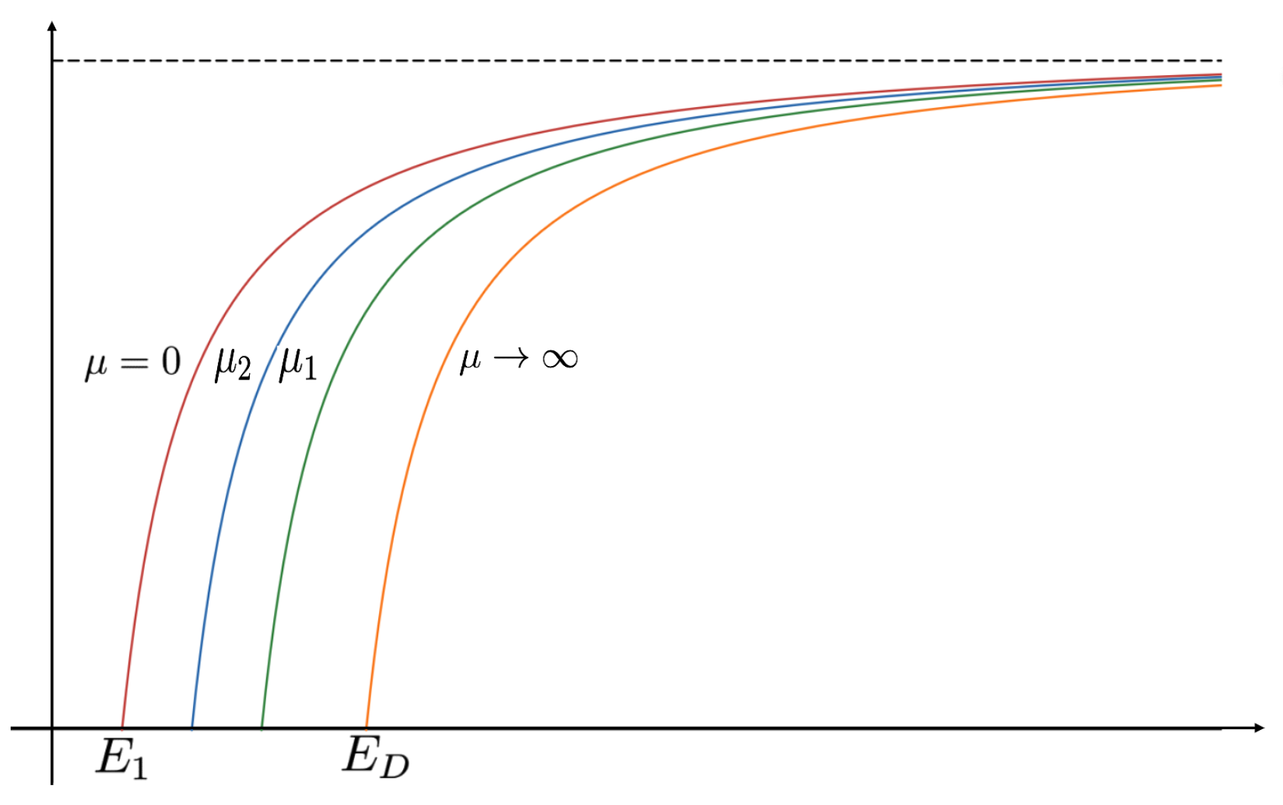
2.2.1. Bifurcation Diagrams for DIE: $g(c,s)=g_1(c,s)=1+\mu c$

For the DIE case, Figure 13 displays the bifurcation diagram of the positive solutions for (7), and Table 6 gives the corresponding ${\lambda }_{min}$-values for various $\mu$-values. We observe that the solution to (7) is always unique with a prediction of extinction for $\lambda \le {\lambda }_{min}$ and unconditional persistence for $\lambda >{\lambda }_{min}$. The bifurcations curve translate to the right, and hence ${\lambda }_{min}$-values increase as $\mu$ increases (see Table 6). The bifurcation curves are again approaching the bifurcation curve corresponding to the completely lethal matrix case (Dirichlet boundary condition) as $\mu \to \infty$. We again highlight that model predictions are drastically affected by PIE strength as measured in $\mu$ for patch sizes with a corresponding $\lambda$-value inside the envelope determined by the red ($\mu =0$) and black ($\mu \to \infty$) curves. For example, for a patch size with corresponding $\lambda ={\lambda }_1=5$, Figure 13 shows model predictions of unconditional persistence when $\mu =0,1,3$, and extinction when $\mu \ge {\mu }^{*}$ for some ${\mu }^{*}>3$.

Figure 13. Bifurcation diagram of positive solutions for (7) with $g_1(c,u)=1+\mu c$ (DIE). Note that the dashed line is for ${\lambda }_1=5$, red represents $\mu =0$, blue $\mu =1$, green $\mu =3$, orange $\mu =10$, and black $\mu \to \infty$.

Table 6. $g_1(c,u)=1+\mu c$.

$\mu$	0	1	3	5	10
${\lambda }_{min}=E_1(1,1+0.1\mu )$	2.95	3.30	3.96	4.53	5.69

2.2.2. Bifurcation Diagrams for +DDE: $g(c,s)=g_2(c,s)=1+\beta u+\mu c$

Figure 14 shows evolution of the bifurcation curves, and Table 7 gives the corresponding ${\lambda }_{min}$-values for the +DDE case with various $\mu$ values. The bifurcation curves translate to the right and approach the bifurcation curve corresponding to the completely lethal matrix case (Dirichlet boundary condition) as $\mu$ increases to ∞. Model predictions are identical to that of the DIE case.

Figure 14. Bifurcation diagram of positive solutions for (7) with $g=g_2(c,u)=1+u+\mu c$ (+DDE with $\beta =1$). Note that red represents $\mu =0$, blue $\mu =1$, green $\mu =3$, orange $\mu =10$, and black $\mu \to \infty$.

Table 7. $g_2(c,u)=1+u+\mu c$ (with $\beta =1$).

$\mu$	0	1	3	5	10
${\lambda }_{min}=E_1(1,1+0.1\mu )$	2.96	3.31	3.96	4.54	5.69

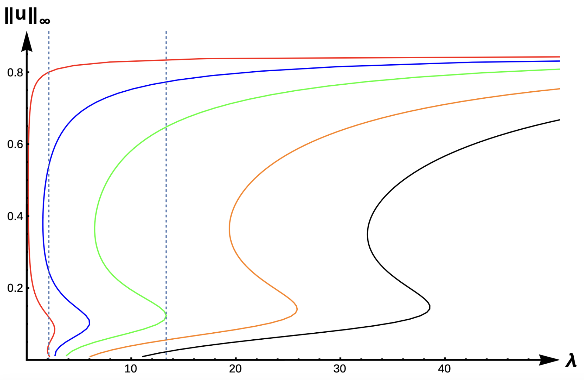
2.2.3. Bifurcation Diagrams for −DDE: $g(c,s)=g_3(c,s)={\displaystyle \frac{1}{1+\beta u}}+\mu c$

Figure 15 and Figure 16 show the bifurcation curves for the −DDE case with strength $\beta =1$ and $\beta =10$, respectively, for various PIE strength values $\mu$. Table 8 and Table 9 give ${\lambda }_{min}$-values, uniqueness regions, and multiplicity regions for various values of $\mu$ for $\beta =1$ and $\beta =10$, respectively. First, we observe that for any fixed DDE strength $\beta$, the bifurcation curves translate to the right as $\mu$ increases, approaching the bifurcation curve of the completely hostile matrix case (Dirichlet boundary condition) when $\mu \to \infty$. 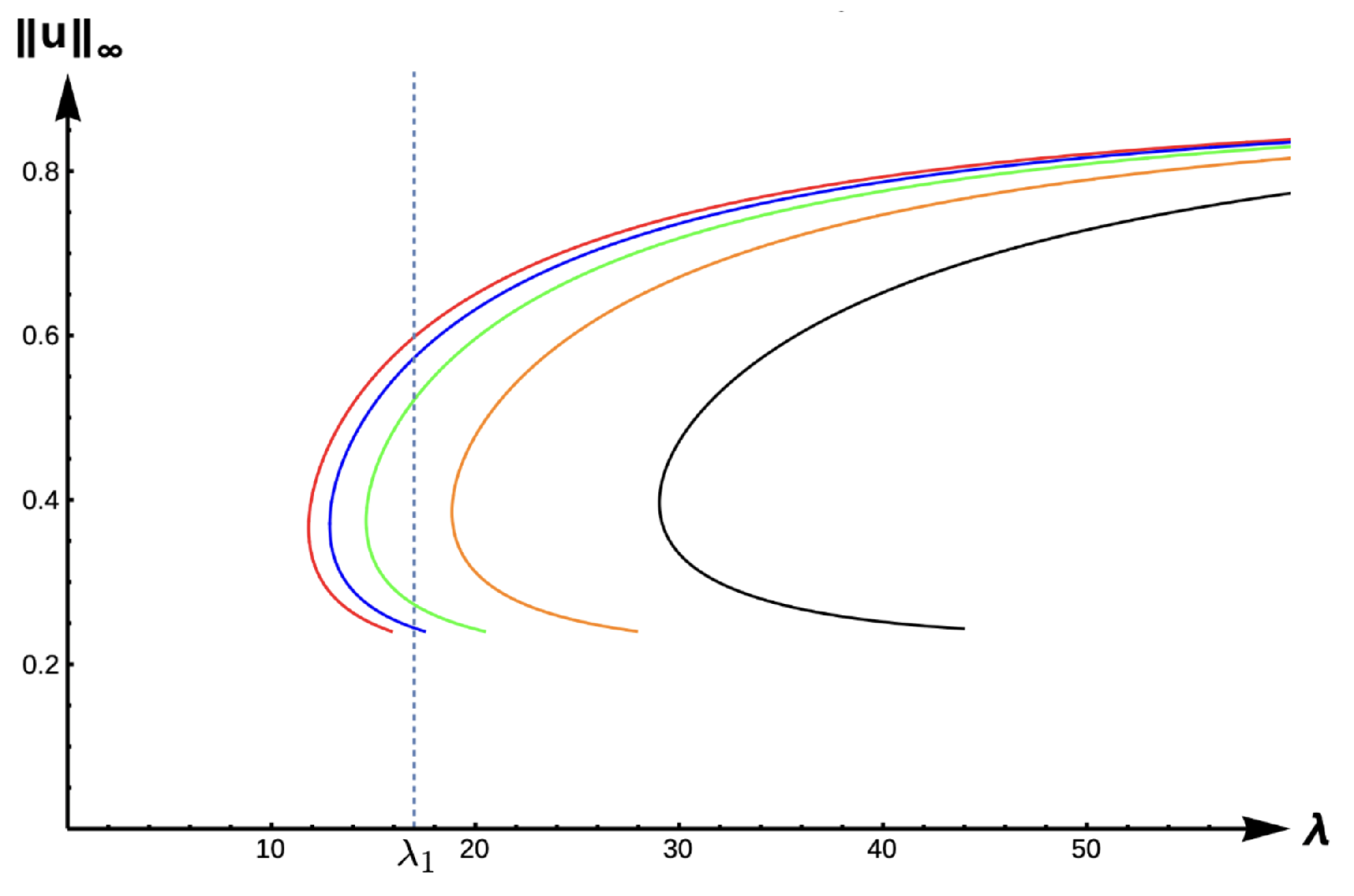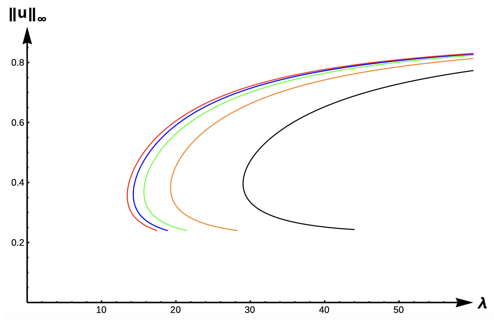For $\beta \approx 0$, model predictions are again similar to those of the previous DIE and +DDE cases. However, when the DDE strength is sufficiently high (as in Figure 16 with $\beta =10$), model predictions become much more interesting. For small PIE strength ($\mu \approx 0$, red, blue, green, and orange in Figure 16), there is a range of patch sizes where a patch-level Allee effect (PAE) is predicted by the model. For a patch with size corresponding to a $\lambda$-value in this range, the model predicts that the population will need to remain above a certain threshold in order to persist. Since the growth term is logistic, this PAE arises solely from the −DDE relationship. Similar cases of PAE have been noted by previous authors for the case when $\mu =0$ (see [18,32,37,42]). However, for higher PIE strength ($\mu \gg 1$, black in Figure 16), no such PAE is present and unconditional persistence is predicted by the model for patch sizes corresponding to $\lambda >{\lambda }_{min}$.

Figure 15. Bifurcation diagram of positive solutions for (7) with $g=g_3(c,u)={\displaystyle \frac{1}{1+u}}+\mu c$ (−DDE with $\beta =1$). Note that red represents $\mu =0$, blue $\mu =1$, green $\mu =3$, orange $\mu =10$, and black $\mu \to \infty$.

Figure 16. Bifurcation diagram of positive solutions for (7) with $g=g_3(c,u)={\displaystyle \frac{1}{1+10u}}+\mu c$ (−DDE with $\beta =10$). Note that the dashed lines represent ${\lambda }_1=1.28$ and ${\lambda }_2=5$, respectively, red represents $\mu =0$, blue $\mu =1$, green $\mu =3$, orange $\mu =10$, and black $\mu \to \infty$.

Table 8. $g_3(c,u)={\displaystyle \frac{1}{1+u}}+\mu c$ (with $\beta =1$).

$\mu$	0	1	3	5	10
${\lambda }_{min}=E_1(1,1+0.1\mu )$	2.94	3.29	3.95	4.53	5.68
Uniqueness Region	$(2.94,\infty )$	$(3.29,\infty )$	$(3.95,\infty )$	$(4.53,\infty )$	$(5.68,\infty )$

Table 9. $g_3(c,u)={\displaystyle \frac{1}{1+10u}}+\mu c$ (with $\beta =10$).

$\mu$	0	1	3	5	10
${\lambda }_{min}$	0.63	1.28	2.63	3.81	5.64
Uniqueness Region	$(2.84,\infty )$	$(3.20,\infty )$	$(3.88,\infty )$	$(4.47,\infty )$	$(5.65,\infty )$
Patch Allee Effect Region	$[0.63,2.84]$	$[1.28,3.20]$	$[2.63,3.88]$	$[3.81,4.47]$	$[5.64,5.65]$

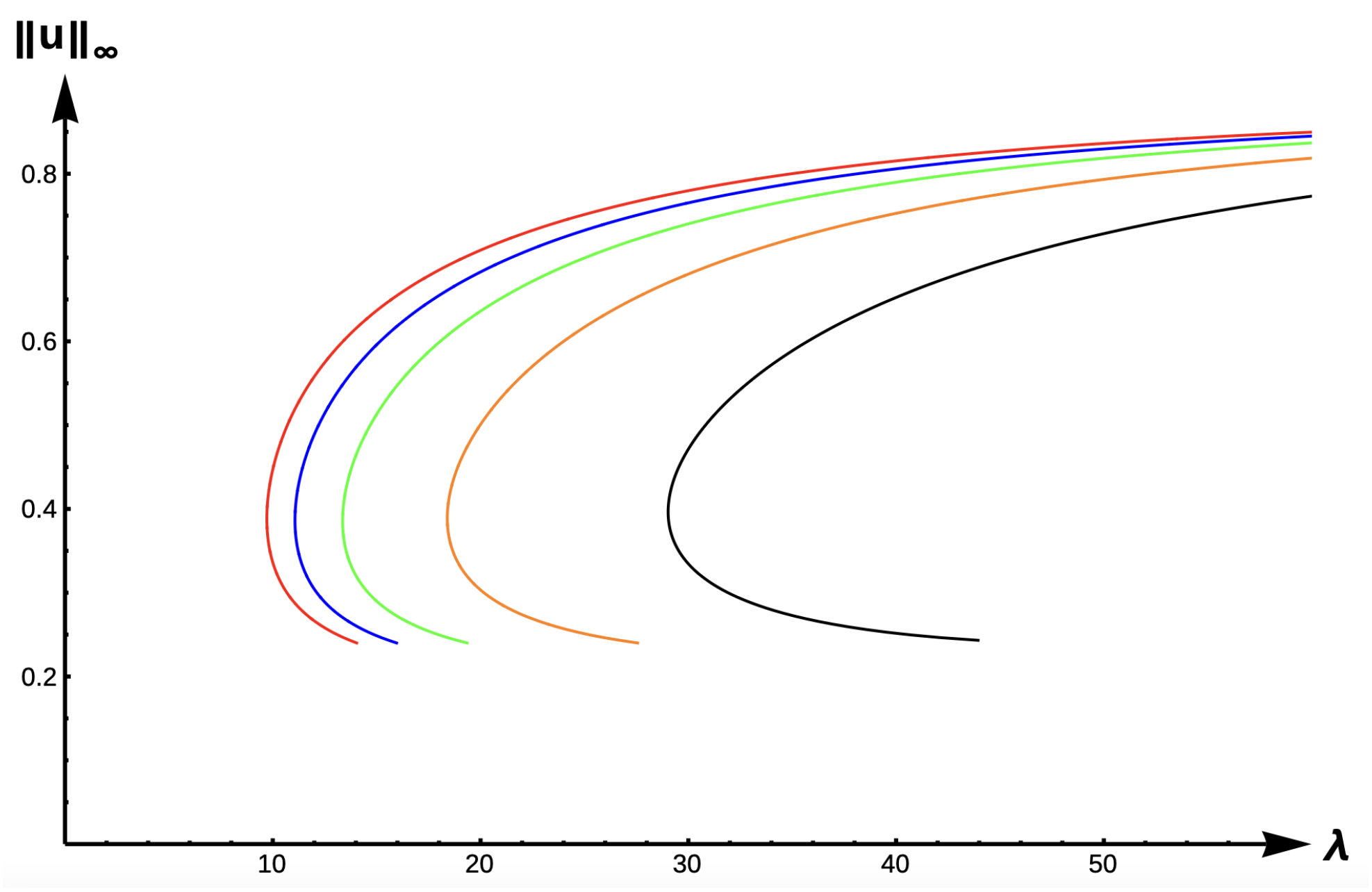
Notice the PIE envelope between the red and black curves in Figure 16 provides a varied range of predictions crucially dependent upon the PIE strength. As an example, a patch with size corresponding to $\lambda ={\lambda }_1$ would have predictions of a PAE for $\mu \approx 0$ and extinction for $\mu \gg 1$. For a patch corresponding to $\lambda ={\lambda }_2$, the model predicts the population is not as sensitive to PIE strength with unconditional persistence predicted for low PIE strength, a PAE for medium levels of PIE, and extinction predicted for high sensitivity to predation. For patches with corresponding ${\lambda }_{min}$ outside of this envelope, predictions of unconditional persistence for $\lambda >{\lambda }_{min}$ and extinction for $\lambda \le {\lambda }_{min}$ are unaffected by PIE altogether.

2.3. Results for Case C: Prey Switching Predation: $h(c,s)=h_3(c,s)={\displaystyle \frac{c{s}^2}{m+s^2}}$

In this subsection, we present the results for the prey switching predation (Holling Type III) case, where we have fixed $c=0.13$ and $m=0.01$. We note that $f(c,s)=s(1-s)-{\displaystyle \frac{c{s}^2}{m+s^2}}$ has two zeros (0 and 0.849) when $c=0.13$ and $m=0.01$. Here, Lemma 3 holds when $\rho \in (0,0.849)$ and $f(c,s)$, $F(c,s)$ have similar shapes to those in Figure 12.

2.3.1. Bifurcation Diagrams for DIE: $g(c,s)=g_1(c,s)=1+\mu c$

For these results, we fix the effective matrix hostility at $\gamma =1$. Figure 17 shows the bifurcation curves for the DIE case for various $\mu$-values. Regardless of the PIE strength, the model predicts one of four outcomes: (1) extinction for $\lambda \le {\lambda }_{min}$, (2) unconditional persistence at a low maximum density level, (3) multiple positive steady states (one at low max density and one at high density), or (4) unconditional persistence at a high maximum density level. Table 10 shows the evolution of the uniqueness region as $\mu$ varies and Table 11 gives multiplicity regions. We also observe that there are three solutions for a certain interval of $\lambda$ between the uniqueness regions. The $\lambda$ interval where the multiplicity occurs translates to the right as $\mu$ increases. The variation in ${\lambda }_{min}$-values is given in Table 12 and we observe that the bifurcation curves translate to the right, approaching the bifurcation curve of the completely lethal matrix case (Dirichlet boundary condition) when $\mu \to \infty$.

Figure 17. Bifurcation diagram of positive solutions for (7) with $g=g_1(c,u)=1+\mu c$ (DIE). Note that the dashed lines represent ${\lambda }_1=16.39$ and ${\lambda }_2=22$, respectively, red represents $\mu =0$, blue $\mu =1$, green $\mu =3$, orange $\mu =10$, and black $\mu \to \infty$.

Table 10. Uniqueness regions.

$\mathit{\mu }$	${\mathit{g}}_1=1+\mathit{\mu }\mathit{c}$	${\mathit{g}}_2=1+\mathit{u}+\mathit{\mu }\mathit{c}$ (With $\mathit{\beta }=1$)
0	$(3.00,14.91)\cup (19.79,\infty )$	$(3.02,16.57)\cup (20.57,\infty )$
1	$(3.45,16.39)\cup (21.37,\infty )$	$(3.47,17.73)\cup (21.98,\infty )$
3	$(4.27,18.79)\cup (23.87,\infty )$	$(4.28,19.67)\cup (24.26,\infty )$
5	$(4.96,20.61)\cup (25.75,\infty )$	$(4.97,21.20)\cup (26.02,\infty )$
10	$(6.25,23.62)\cup (28.88,\infty )$	$(6.25,23.87)\cup (29.00,\infty )$

Table 11. Multiplicity regions.

$\mathit{\mu }$	${\mathit{g}}_1=1+\mathit{\mu }\mathit{c}$	${\mathit{g}}_2=1+\mathit{u}+\mathit{\mu }\mathit{c}$ (With $\mathit{\beta }=1$)
0	$[14.91,19.79]$	$[16.57,20.57]$
1	$[16.39,21.37]$	$[17.73,21.98]$
3	$[18.79,23.87]$	$[19.67,24.26]$
5	$[20.61,25.75]$	$[21.20,26.02]$
10	$[23.62,28.88]$	$[23.87,29.00]$

Table 12. Variation in ${\lambda }_{min}=E_1(1,1+0.1\mu )$.

$\mu$	0	1	3	5	10
$g_1(c,u)=1+\mu c$	3.00	3.45	4.27	4.96	6.25
$g_2(c,u)=1+u+\mu c$ (with $\beta =1$)	3.02	3.47	4.28	4.97	6.25

As in previous cases, the envelope of $\lambda$-values for which model predictions are especially sensitive to PIE strength is given between the red and black curves in Figure 17. To highlight the effects of PIE, we first consider the example of a patch with size corresponding to $\lambda ={\lambda }_1$ in Figure 17. For a small PIE strength ($\mu \approx 0$), there is a non-Allee type bi-stability as denoted in case (3) above; however, for large PIE strength, unconditional persistence at a low density level (as in case (2) above) is predicted. For a larger patch with size corresponding to $\lambda ={\lambda }_2$, cases (2)–(4) from above are possible as the PIE strength increases. Again, the sensitivity of the predation–emigration relationship causes vast population dynamical outcomes, even for the same patch size and matrix quality.

2.3.2. Bifurcation Diagrams for +DDE: $g(c,s)=g_2(c,s)=1+\beta u+\mu c$, $\gamma =1$

For the +DDE case, we again fix $\gamma =1$. Figure 18 shows how the bifurcation curves translate to the right as the PIE strength $\mu$ increases. Corresponding ${\lambda }_{min}$-values are given in Table 12, while Table 10 shows the variation in the uniqueness regions as $\mu$ changes. The $\lambda$-interval where the multiplicity occurs translates to the right as $\mu$ increases. Model predictions are identical to those of the DIE case.

Figure 18. Bifurcation diagram of positive solutions for (7) with $g=g_2(c,u)=1+u+\mu c$ (+DDE with $\beta =1$). Note that red represents $\mu =0$, blue $\mu =1$, green $\mu =3$, orange $\mu =10$, and black $\mu \to \infty$.

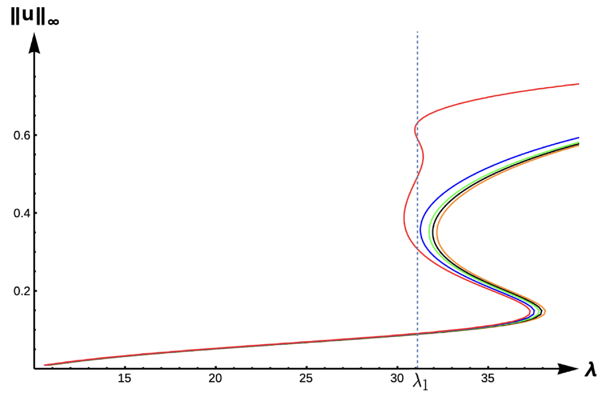
2.3.3. Bifurcation Diagrams for −DDE: $g(c,s)=g_3(c,s)={\displaystyle \frac{1}{1+\beta u}}+\mu c$

For the final case of −DDE, Figure 19, Figure 20 and Figure 21 show the evolution of bifurcation curves for $\beta =1,30,40$, respectively, as $\mu$ varies. Table 13 gives uniqueness regions, Table 14 gives multiplicity regions, Table 15 gives patch level Alllee effect regions, and Table 16 provide uniqueness regions and ${\lambda }_{min}$-values, respectively, as $\mu$ varies. The case of low DDE strength ($\beta =1$) gives a scenario that is identical to the DIE and +DDE cases but with a leftward translation in the curves as illustrated in Figure 19. However, the envelope created by the red and black curves in Figure 20 and Figure 21 show a myriad of possible model predictions.

Figure 19. Bifurcation diagram of positive solutions for (7) with $g=g_3(c,u)={\displaystyle \frac{1}{1+u}}+\mu c$ (−DDE with $\beta =1$). Note that red represents $\mu =0$, blue $\mu =1$, green $\mu =3$, orange $\mu =10$, and black $\mu \to \infty$.

Figure 20. Bifurcation diagram of positive solutions for (7) with $g=g_3(c,u)={\displaystyle \frac{1}{1+30u}}+\mu c$ (−DDE with $\beta =30$). Note that red represents $\mu =0$, blue $\mu =1$, green $\mu =3$, orange $\mu =10$, and black $\mu \to \infty$.

Figure 21. Bifurcation diagram of positive solutions for (7) with $g=g_3(c,u)={\displaystyle \frac{1}{1+40u}}+\mu c$ (−DDE with $\beta =40$). Note that the dashed lines represent ${\lambda }_1=2.11$ & ${\lambda }_2=13.35$, respectively, and red represents $\mu =0$, blue $\mu =1$, green $\mu =3$, orange $\mu =10$, and black $\mu \to \infty$.

Table 13. $g_3(c,u)={\displaystyle \frac{1}{1+\beta u}}+\mu c$, uniqueness regions.

$\mathit{\mu }$	$\mathit{\beta }=1$	$\mathit{\beta }=30$	$\mathit{\beta }=40$
0	$(2.98,12.67)\cup (18.91,\infty )$	$(4.00,\infty )$	$(2.68,\infty )$
1	$(3.43,14.66)\cup (20.70,\infty )$	$(2.40,4.32)\cup (6.37,\infty )$	$(6.02,\infty )$
3	$(4.25,17.73)\cup (23.46,\infty )$	$(3.85,7.01)\cup (14.76,\infty )$	$(3.72,6.50)\cup (13.35,\infty )$
5	$(4.95,19.93)\cup (25.48,\infty )$	$(4.64,12.01)\cup (19.75,\infty )$	$(4.55,11.49)\cup (18.75,\infty )$
10	$(6.24,23.34)\cup (28.77,\infty )$	$(6.09,19.73)\cup (26.35,\infty )$	$(6.04,19.38)\cup (25.88,\infty )$

Table 14. $g_3(c,u)={\displaystyle \frac{1}{1+\beta u}}+\mu c$, multiplicity region.

$\mathit{\mu }$	$\mathit{\beta }=1$	$\mathit{\beta }=30$	$\mathit{\beta }=40$
0	$[12.67,18.91]$	(2.37, 4.00]	$(2.19,2.68]$
1	$[14.66,20.70]$	$[4.32,6.37]$	$[2.73,6.02]$
3	$[17.73,23.46]$	$[7.01,14.76]$	$[6.50,3.35]$
5	$[19.93,25.48]$	$[12.01,19.75]$	$[11.49,18.75]$
10	$[23.34,28.77]$	$[19.73,26.35]$	$[19.38,25.88]$

Table 15. $g_3(c,u)={\displaystyle \frac{1}{1+\beta u}}+\mu c$, Patch Allee effect region.

$\mathit{\mu }$	$\mathit{\beta }=1$	$\mathit{\beta }=30$	$\mathit{\beta }=40$
0	None	$[0.25,2.37]$	$[0.14,2.19]$
1	None	$[1.86,2.90]$	$[1.55,2.73]$
3	None	None	None
5	None	None	None
10	None	None	None

Table 16. $g_3(c,u)={\displaystyle \frac{1}{1+\beta u}}+\mu c$, ${\lambda }_{min}$.

$\mu$	0	1	3	5	10
$\beta =1$	2.98	3.43	4.25	4.95	6.24
$\beta =30$	2.37	2.40	3.85	4.64	6.09
$\beta =40$	2.19	2.73	3.72	4.55	6.04

In the case of medium DDE strength ($\beta =30$ in Figure 20), potential model predictions include (1) extinction for $\lambda \le {\lambda }_{min}$, (2) a PAE, (3) unconditional persistence at a low maximum density level, (4) non-Allee effect type bi-stability (one positive steady state at low max density and one at high density), or (5) unconditional persistence at a high maximum density level. For the high DDE strength case ($\beta =40$), all five of these dynamical outcomes are possible with the addition of a scenario as illustrated at $\lambda ={\lambda }_1$ in the red curve of Figure 21. For this $\lambda$-value, a PAE occurs and persistence is possible at either a high maximum density or a small maximum density level. Increasing the PIE strength for this patch size will change model prediction to that of a PAE, followed by extinction for sufficiently high PIE strength. However, for a patch with size corresponding to $\lambda ={\lambda }_2$, outcomes (2)–(5) above are possible as the PIE sensitivity increases.

Next, we explore the effects of matrix hostility by considering the case with high DDE strength ($\beta =80$) and high matrix hostility ($\gamma =26$). Figure 22 illustrates the effect that extreme matrix hostility has on the model predictions, showing a new dynamical scenario at $\lambda ={\lambda }_1$. At this value, there are five positive solutions to the steady-state problem, showing a very complex situation. Here, persistence is possible but with a variety of different maximum density levels. Figure 23 shows the evolution of bifurcation curves for $\mu \approx 0$ as the PIE strength increases.

Figure 22. Bifurcation diagram of positive solutions for (7) with $g=g_3(c,u)={\displaystyle \frac{1}{1+80u}}+\mu c$ (−DDE with $\beta =80$) and $\gamma =26$. Note that the dashed line represents ${\lambda }_1=31.10$, red represents $\mu =0$, blue $\mu =1$, green $\mu =3$, orange $\mu =10$, and black $\mu \to \infty$.

Figure 23. Bifurcation diagram of positive solutions for (7) with $g=g_3(c,u)={\displaystyle \frac{1}{1+80u}}+\mu c$ (−DDE with $\beta =80$) and $\gamma =26$. Note that red represents $\mu =0$, blue $\mu =0.003$, green $\mu =0.005$, purple $\mu =0.01$, and orange $\mu =0.02$.

3. Preliminaries

In this section, we introduce definitions of the (strict) subsolution and (strict) supersolution of (1), state a sub-supersolution theorem that is used to prove the existence and multiplicity results of positive solutions, and state a lemma which we employ to numerically generate bifurcation curves.

By a subsolution of (1), we mean $\psi \in C^2(\Omega )\cap C^1\left(\overline{\Omega }\right)$ that satisfies

$$\left\{\begin{array}{c}-\Delta \psi \le \lambda f(c,\psi );\Omega \\ {\displaystyle \frac{\partial \psi }{\partial \eta }}+\gamma \sqrt{\lambda }g(c,\psi )\psi \le 0;\partial \Omega .\end{array}\right.$$

By a supersolution of (1), we mean $Z\in C^2(\Omega )\cap C^1\left(\overline{\Omega }\right)$ that satisfies

$$\left\{\begin{array}{c}-\Delta Z\ge \lambda f(c,Z);\Omega \\ {\displaystyle \frac{\partial Z}{\partial \eta }}+\gamma \sqrt{\lambda }g(c,Z)Z\ge 0;\partial \Omega .\end{array}\right.$$

By a strict subsolution (supersolution) of (1), we mean a subsolution (supersolution) which is not a solution. Then, the following results hold (see [43,44,45]):

Lemma 1.

Let ψ and Z be a subsolution and a supersolution of (1), respectively, such that $\psi \le Z$. Then, (1) has a solution $u\in C^2(\Omega )\cap C^1\left(\overline{\Omega }\right)$ such that $u\in [\psi ,Z]$.

Lemma 2.

Let ${\psi }_1$ and $Z_2$ be a subsolution and a supersolution of (1), respectively, such that ${\psi }_1\le Z_2$. Let ${\psi }_2$ and $Z_1$ be a strict subsolution and a strict supersolution of (1), respectively, such that ${\psi }_2$, $Z_1\in [{\psi }_1,Z_2]$ and ${\psi }_2\nleqq Z_1$. Then, (1) has at least three solutions, $u_1$, $u_2$ and $u_3$ where $u_i\in [{\psi }_i,Z_i];i=1,2$ and $u_3\in [{\psi }_1,Z_2]\setminus ([{\psi }_1,Z_1]\cup [{\psi }_2,Z_2])$.

Let u be a positive solution of (7) when $\Omega =(0,1)$. Since $g(c,s)s$ is increasing for all $s>0,$ it follows that u must be symmetric about $x={\displaystyle \frac{1}{2}}$ and has the shape as in Figure 24 below (see [32]). Let $u\left(0\right)=u\left(1\right)=q$ and ${\parallel u\parallel }_{\infty }=u\left({\displaystyle \frac{1}{2}}\right)=\rho$.

Figure 24. The shape of the symmetric positive solutions of (7).

Then the following result holds:

Lemma 3.

(See [32]). For $\lambda >0,$ (7) has a positive solution u such that ${\parallel u\parallel }_{\infty }=\rho$, $u\left(0\right)=u\left(1\right)=q$, with $0<q<\rho$ if and only if λ, ρ, and q satisfy

$$\lambda =2{\left({\int }_{q\left(\rho \right)}^{\rho }{\displaystyle \frac{ds}{\sqrt[]{F(c,\rho )-F(c,s)}}}\right)}^2$$

(8)

and

$$2[F(c,\rho )-F(c,q)]={\gamma }^2{\left(g(c,q)\right)}^2{q}^2$$

(9)

where $f(c,s)=s(1-s)-h(c,s)$ and $F(c,s)={\int }_0^{s}f(c,r)dr$.

Remark 4.

We provide the proof of Lemma 3 in the appendix for the convenience of the reader.

Next, we briefly explain how we obtain bifurcation curves using (8)–(9). Let $z_0$ be the unique positive falling zero of f and $x_i=\theta +{\displaystyle \frac{(z_0-\theta )}{n+1}}i;i=1,...,n$ for some $n\ge 1$, where $\theta$ is the smallest positive zero of F when $h(c,s)=h_1(c,s)$ and $\theta =0$ when $h(c,s)=h_2(c,s)$ or $h(c,s)=h_3(c,s)$. Letting $\rho =x_1$, we numerically solve the Equation (9) for q using the FindRoot command in Mathematica. The values of q and $\rho$ are substituted into (8) to find the corresponding value of $\lambda$. Repeating this procedure for $\rho =x_i$, $i=2,......,n$, we obtain $(\lambda ,\rho )$ points for the bifurcation diagram.

We note that, in our study, when $f(c,0)=0$, the branch of positive solutions bifurcates from $(\lambda ,0)$ at $E_1(M,g_0(\mu ,c),\gamma )$, where $E_1(M,g_0(\mu ,c),\gamma )$ is the principal (first positive) eigenvalue of

$$\left\{\begin{array}{c}-\varphi ″=EM\varphi ;(0,1)\\ -\varphi \prime \left(0\right)+\gamma \sqrt{E}{g}_0(\mu ,c)\varphi \left(0\right)=0\\ {\varphi }^{\prime }\left(1\right)+\gamma \sqrt{E}{g}_0(\mu ,c)\varphi \left(1\right)=0\end{array}\right.$$

(10)

with an eigenfunction $\varphi >0;[0,1]$. Here, $M=1-c$ when $h=h_2$ and $M=1$ when $h=h_3$.

4. Construction of Subsolutions and Supersolutions to Prove Theorems 1–6

Here, we state a couple of eigenvalue problems which are crucial to our proofs and recall some properties of their respective principal eigenvalues. For $M,b,\lambda ,\gamma >0$, let ${\sigma }_0={\sigma }_0(M,b,\lambda ,\gamma )$ be the principal eigenvalue, ${\varphi }_0>0;\overline{\Omega }$ be the corresponding normalized eigenfunction of

$$\left\{\begin{array}{c}-\Delta {\varphi }_0-\lambda M{\varphi }_0={\sigma }_0{\varphi }_0;\Omega \\ {\displaystyle \frac{\partial {\varphi }_0}{\partial \eta }}+\gamma \sqrt{\lambda }b{\varphi }_0=0;\partial \Omega \end{array}\right.$$

(11)

and let ${\sigma }_1={\sigma }_1(M,b,\lambda ,\gamma )$ be the principal eigenvalue and ${\varphi }_1>0;\overline{\Omega }$ be the corresponding normalized eigenfunction of

$$\left\{\begin{array}{c}-\Delta {\varphi }_1-\lambda M{\varphi }_1={\sigma }_1{\varphi }_1;\Omega \\ {\displaystyle \frac{\partial {\varphi }_1}{\partial \eta }}+\gamma \sqrt{\lambda }b{\varphi }_1={\sigma }_1{\varphi }_1;\partial \Omega .\end{array}\right.$$

(12)

Note that the existence of both principle eigenvalues is standard (see [15,46]). For simplicity of notation, we denote ${\tilde{\sigma }}_i={\sigma }_i(1-c,g_0(\mu ,c),\lambda ,\gamma )$ with corresponding normalized eigenfunction ${\tilde{\varphi }}_i$ for $i=0,1$.

The following lemma gives several useful properties of ${\sigma }_i(M,b,\lambda ,\gamma )$ and $E_1(M,b,\gamma )$ (see [15,46,47]).

Lemma 4.

Let $M,\gamma ,b>0$, ${\sigma }_0(M,b,\lambda ,\gamma )$ denote the principal eigenvalue of (11), ${\sigma }_1(M,b,\lambda ,\gamma )$ the principal eigenvalue of (12), and $E_1(M,b,\gamma )$ the principal eigenvalue of (2). Then, we have the following for $i=0,1$:

(1) 

${\sigma }_i(M,b,\lambda ,\gamma )\ge 0$ for $\lambda \le E_1(M,b,\gamma )$.

(2) 

${\sigma }_i(M,b,\lambda ,\gamma )<0$ for $\lambda >E_1(M,b,\gamma )$.

(3) 

${\sigma }_i(M,b,\lambda ,\gamma )$ is decreasing in M and increasing in b and γ.

(4) 

$\mathit{sgn}\left({\sigma }_0(M,b,\lambda ,\gamma )\right)=\mathit{sgn}\left({\sigma }_1(M,b,\lambda ,\gamma )\right)$.

(5) 

$E_1(M,b,\gamma )$ is decreasing in M and increasing in b and γ.

Now, we present the construction of several crucial sub- and supersolutions for (2).

• Construction of a subsolution ${\psi }_1$ when $\lambda >E_1(M,g_0(\mu ,c),\gamma )$ for $\gamma >0$, $h=h_2$ or $h=h_3$ and $g=g_1$ (DIE), $g=g_2$ (+DDE) or $g=g_3$ (−DDE), where $M=1-c$ when $h=h_2$ and $M=1$ when $h=h_3$.

For a fixed $\lambda >0$, recall that ${\tilde{\sigma }}_1={\sigma }_1(M,g_0(\mu ,c),\lambda ,\gamma )$ is the principal eigenvalue and ${\tilde{\varphi }}_1>0;\overline{\Omega }$ the corresponding normalized eigenfunction of (12). We note that ${\tilde{\sigma }}_1<0$ for $\lambda >E_1(M,g_0(\mu ,c),\gamma )$. Let ${\psi }_1:={\delta }_1{\tilde{\varphi }}_1$ for ${\delta }_1>0$ and $l\left(s\right)=({\tilde{\sigma }}_1+\lambda M)s-\lambda f(c,s).$ Then, we have $l\left(0\right)=0$ and $l^{\prime }\left(0\right)=({\tilde{\sigma }}_1+\lambda M)-\lambda f^{\prime }(c,0)={\tilde{\sigma }}_1<0$ since $f^{\prime }(c,0)=M$. Therefore, $l\left(s\right)<0; s\approx 0$. This implies that

$$\begin{array}{cc}\hfill -\Delta {\psi }_1& ={\delta }_1(\lambda +{\tilde{\sigma }}_1){\tilde{\varphi }}_1<\lambda f(c,{\delta }_1{\tilde{\varphi }}_1)=\lambda f(c,{\psi }_1);\Omega \hfill \end{array}$$

for ${\delta }_1\approx 0$. We also have

$$\begin{array}{cc}\hfill {\displaystyle \frac{\partial {\psi }_1}{\partial \eta }}+\gamma \sqrt{\lambda }g(c,{\psi }_1){\psi }_1& ={\delta }_1\left({\displaystyle \frac{\partial {\tilde{\varphi }}_1}{\partial \eta }}+\gamma \sqrt{\lambda }g(c,{\delta }_1{\tilde{\varphi }}_1){\tilde{\varphi }}_1\right)\hfill \\ \hfill & ={\delta }_1\left(-\gamma \sqrt{\lambda }b{\tilde{\varphi }}_1+{\tilde{\sigma }}_1{\tilde{\varphi }}_1+\gamma \sqrt{\lambda }g(c,{\delta }_1{\tilde{\varphi }}_1){\tilde{\varphi }}_1\right)\hfill \\ \hfill & ={\delta }_1{\tilde{\varphi }}_1\left(\gamma \sqrt{\lambda }(g(c,{\delta }_1{\tilde{\varphi }}_1)-g_0(\mu ,c))+{\tilde{\sigma }}_1\right)\hfill \\ \hfill & <0;\partial \Omega \hfill \end{array}$$

for ${\delta }_1\approx 0$ since $g(c,{\delta }_1{\tilde{\varphi }}_1)\approx g_0(\mu ,c)$ and ${\tilde{\sigma }}_1<0$ for $\lambda >E_1(M,g_0(\mu ,c),\gamma ).$ Hence, ${\psi }_1$ is a subsolution of (1) for $\lambda >E_1(M,g_0(\mu ,c),\gamma )$.

• Construction of a subsolution ${\psi }_2$ when $\lambda >E_1^D$ such that $\parallel {\psi }_2{\parallel }_{\infty }⟶1$ as $\lambda ⟶\infty$ for $\gamma >0$, $h=h_2$ and $g=g_1$ (DIE) or $g=g_2$ (+DDE).

Consider the following problem:

$$\left\{\begin{array}{c}-\Delta w=\lambda \left[w\right(1-w)-cw];\Omega \\ w=0;\partial \Omega .\end{array}\right.$$

(13)

Let $w_{\lambda }$ be the unique positive solution of (13) for $\lambda >E_1^D$ (see [15]), where $E_1^D$ is the principal eigenvalue of (4).

We note that $\parallel w_{\lambda }{\parallel }_{\infty }\to z_0$ as $\lambda \to \infty .$ Let ${\psi }_2:=w_{\lambda }$. Then, we have $-\Delta {\psi }_2=\lambda f(c,{\psi }_2);\Omega .$ Also,

$$\begin{array}{c}\hfill {\displaystyle \frac{\partial {\psi }_2}{\partial \eta }}+\gamma \sqrt{\lambda }g(c,{\psi }_2){\psi }_2={\displaystyle \frac{\partial w_{\lambda }}{\partial \eta }}<0;\partial \Omega \end{array}$$

by the Hopf maximum principle. Therefore, ${\psi }_2$ is a subsolution of (1) for $\lambda >E_1^D$ such that $\parallel {\psi }_2{\parallel }_{\infty }⟶z_0$ as $\lambda ⟶\infty$.

• Construction of a strict subsolution ${\psi }_3$ in $\left[{\lambda }^{*},E_1(1-c,g_0(\mu ,c),\gamma )\right]$ when $\gamma >0$, $h=h_2$, and $g=g_3(-\mathbf{DDE})$ when $\beta >{\beta }_1\left(\mu \right)$ for some ${\beta }_1\left(\mu \right)>0.$

Let $\lambda \in I$ where I is as in (3). Choose $M=1-c$ and $b={\displaystyle \frac{g_0(\mu ,c)+\mu c}{2}}$ in (11). Next, for a fixed $\lambda >0$, let ${\overline{\sigma }}_0={\sigma }_0(1-c,{\displaystyle \frac{g_0(\mu ,c)+\mu c}{2}},\lambda ,\gamma )$ be the principal eigenvalue and ${\overline{\varphi }}_0>0;\overline{\Omega }$ be the corresponding normalized eigenfunction of (11). We note that ${\overline{\sigma }}_0<0$ when $\lambda >E_1(1-c,{\displaystyle \frac{g_0(\mu ,c)+\mu c}{2}},\gamma )$. Define $H\left(s\right):=(\lambda (1-c)+{\overline{\sigma }}_0)s-\lambda f(c,s)$ for $\lambda \ge {\lambda }^{*}$. Then, $H\left(0\right)=0$ and $H^{\prime }\left(0\right)={\overline{\sigma }}_0<0$ since $f(c,0)=0$, $f^{\prime }(c,0)=1-c$, and ${\overline{\sigma }}_0<0$. This implies that $H\left(s\right)<0$ for $s\approx 0$. Let $s_{\lambda }\in (0,z_0)$ be such that

$$H\left(s\right)=(\lambda (1-c)+{\overline{\sigma }}_0)s-\lambda f(c,s)<0;\mathrm{for} \mathrm{all}s\in (0,s_{\lambda }].$$

(14)

Next, we define $K=K(a,\Omega ):=\underset{\lambda \in I}{min}\underset{\overline{\Omega }}{min}\left\{{\delta }_4{\overline{\varphi }}_0\right\}$ where ${\delta }_4:=\underset{\lambda \in I}{min}\left\{s_{\lambda }\right\}$. Observe that $0<{\delta }_4<z_0$, and $\parallel {\overline{\varphi }}_0{\parallel }_{\infty }\le 1$ implies that $K<z_0.$ Let $\lambda \in I$ and define ${\psi }_3:={\delta }_4{\overline{\varphi }}_0.$ From (14), we have

$$-\Delta {\psi }_3=-{\delta }_4\Delta {\overline{\varphi }}_0={\delta }_4(\lambda (1-c)+{\overline{\sigma }}_0){\overline{\varphi }}_0<\lambda f(c,{\delta }_4{\overline{\varphi }}_0)=\lambda f(c,{\psi }_3);\Omega .$$

Next, since ${\delta }_4{\overline{\varphi }}_0\ge K$, we have

$$\begin{array}{cc}\hfill 1+\beta {\delta }_4{\overline{\varphi }}_0& \ge 1+\beta K;\partial \Omega .\hfill \end{array}$$

This implies that

$$\begin{array}{cc}\hfill {\displaystyle \frac{1}{1+\beta {\delta }_4{\overline{\varphi }}_0}}+\mu c-\left({\displaystyle \frac{g_0(\mu ,c)+\mu c}{2}}\right)& \le {\displaystyle \frac{1}{1+\beta K}}+\mu c-\left({\displaystyle \frac{g_0(\mu ,c)+\mu c}{2}}\right);\partial \Omega .\hfill \end{array}$$

(15)

Let ${\beta }_1:={\beta }_1\left(\mu \right)$ be such that

$${\displaystyle \frac{1}{1+{\beta }_{1}K}}+\mu c-\left({\displaystyle \frac{g_0(\mu ,c)+\mu c}{2}}\right)=0.$$

This implies that ${\beta }_1={\displaystyle \frac{1}{K}}.$ Observe that ${\beta }_1>0$ and

$${\displaystyle \frac{1}{1+\beta K}}+\mu c-\left({\displaystyle \frac{g_0(\mu ,c)+\mu c}{2}}\right)<0$$

for $\beta >{\beta }_1.$ Now, for $\beta >{\beta }_1$, we have

$$\begin{array}{cc}\hfill {\displaystyle \frac{\partial {\psi }_3}{\partial \eta }}+\gamma \sqrt{\lambda }g(c,{\psi }_3){\psi }_3& ={\delta }_4\left({\displaystyle \frac{\partial {\overline{\varphi }}_0}{\partial \eta }}+\gamma \sqrt{\lambda }g(c,{\delta }_4{\overline{\varphi }}_0){\overline{\varphi }}_0\right)\hfill \\ \hfill & ={\delta }_4\gamma \sqrt{\lambda }{\overline{\varphi }}_0\left({\displaystyle \frac{1}{1+\beta {\delta }_4{\overline{\varphi }}_0}}+\mu c-\left({\displaystyle \frac{g_0(\mu ,c)+\mu c}{2}}\right)\right)\hfill \\ \hfill & <0;\partial \Omega \hfill \end{array}$$

by (15). Hence, ${\psi }_3$ is a strict subsolution of (1) for $\lambda \in I$ and $\beta >{\beta }_1.$

• Construction of a strict subsolution ${\psi }_4$ when $\left(H_1\right)$ & $\left(H_2\right)$ hold for $\lambda \in \left({\displaystyle \frac{2bN{C}_N}{R^{2}f(c,b)}},{\displaystyle \frac{2r_{2}N}{f(c,b)R^2}}\right)$.

Let $\tilde{g}\in C^1\left([0,\infty )\right)$ be such that $\tilde{g}$ is non-decreasing on $[0,r_2),0\le \tilde{g}\left(s\right)\le f(c,s)$ on $[0,r_1)$ and $\tilde{g}\left(s\right)=f(c,s)$ on $[r_1,r_2).$ Then, the following boundary value problem

$$\left\{\begin{array}{c}-\Delta w=\lambda \tilde{g}\left(w\right);\Omega \\ u=0;\partial \Omega ,\end{array}\right.$$

has a solution ${\tilde{w}}_{\lambda }\ge 0$ such that $\parallel {\tilde{w}}_{\lambda }{\parallel }_{\infty }\ge b$ for $\lambda \in \left({\displaystyle \frac{2bN{C}_N}{R^{2}f(c,b)}},{\displaystyle \frac{2r_{2}N}{f(c,b)R^2}}\right)$ provided $\left(H_3\right)$ and $\left(H_4\right)$ are satisfied (see [33]). Let ${\psi }_4:={\tilde{w}}_{\lambda }.$ Since $\tilde{g}\left(s\right)\le f(c,s)$ on $[0,z_0)$ and ${\displaystyle \frac{\partial {\tilde{w}}_{\lambda }}{\partial \eta }}<0$ on $\partial \Omega$ by the Hopf maximum principle, it is easy to show that ${\psi }_4$ is a strict subsolution of (1) for $\lambda \in \left({\displaystyle \frac{2bN{C}_N}{R^{2}f(c,b)}},{\displaystyle \frac{2r_{2}N}{f(c,b)R^2}}\right)$.

• Construction of a strict supersolution $Z_1$ for $\lambda >0$, $\gamma >0$, $h=h_1$, $h=h_2$, or $h=h_3$, and any form of g.
• $Z_1=z_0$ is a global supersolution of (1) for all $\lambda >0$.
• Construction of a strict supersolution $Z_2$ for $\lambda \in (0,E_1(M,g_0(\mu ,c),\gamma ))$, for $\gamma >0$, $h=h_2$ or $h=h_3$ and any form of g where $M=1-c$ when $h=h_2$ and $M=1$ when $h=h_3$.

For a fixed $\lambda >0$, recall ${\tilde{\sigma }}_1={\sigma }_1(M,g_0(\mu ,c),\lambda ,\gamma )$ is the principal eigenvalue and ${\tilde{\varphi }}_1>0;\overline{\Omega }$ the corresponding normalized eigenfunction of (12). We note that ${\tilde{\sigma }}_1>0$ for $\lambda <E_1(M,g_0(\mu ,c),\gamma )$ (see Lemma 4). Let $Z_2:=m_2{\tilde{\varphi }}_1$ and $l\left(s\right)=({\tilde{\sigma }}_1+\lambda M)s-\lambda f(c,s).$ Since $f(c,0)=0$ and $f^{\prime }(c,0)=M$, we have $l\left(0\right)=0$ and $l^{\prime }\left(0\right)=({\tilde{\sigma }}_1+\lambda M)-\lambda f^{\prime }(c,0)={\tilde{\sigma }}_1>0$ giving that $l\left(s\right)>0$ for $s\approx 0$. This implies that

$$\begin{array}{cc}\hfill -\Delta Z_2& =m_2(\lambda M+{\tilde{\sigma }}_1){\tilde{\varphi }}_1>\lambda f(c,m_2{\tilde{\varphi }}_1)=\lambda f(c,Z_2);\Omega \hfill \end{array}$$

and

$$\begin{array}{cc}\hfill {\displaystyle \frac{\partial Z_2}{\partial \eta }}+\gamma \sqrt{\lambda }g(c,Z_2)Z_2& =m_2\left({\displaystyle \frac{\partial {\tilde{\varphi }}_1}{\partial \eta }}+\gamma \sqrt{\lambda }g(c,m_2{\tilde{\varphi }}_1){\tilde{\varphi }}_1\right)\hfill \\ \hfill & =m_2\left(-\gamma \sqrt{\lambda }{g}_0(\mu ,c){\tilde{\varphi }}_1+{\tilde{\sigma }}_1{\tilde{\varphi }}_1+\gamma \sqrt{\lambda }g(c,m_2{\tilde{\varphi }}_1){\tilde{\varphi }}_1\right)\hfill \\ \hfill & =m_2{\tilde{\varphi }}_1\left(\gamma \sqrt{\lambda }(g(c,m_2{\tilde{\varphi }}_1)-g_0(\mu ,c))+{\tilde{\sigma }}_1\right)\hfill \\ \hfill & >0;\partial \Omega \hfill \end{array}$$

for $m_2\approx 0$ since $g(c,0)=g_0(\mu ,c).$ Hence, $Z_2$ is a strict supersolution of (1) for $\lambda <E_1(M,g_0(\mu ,c),\gamma )$ and $m_2\approx 0$.

• Construction of a small supersolution $Z_3$ for $\lambda >E_1(1-c,g_0(\mu ,c),\gamma )$ and $\lambda \approx E_1(1-c,g_0(\mu ,c),\gamma )$ when $h=h_2$ and $g=g_1$ (DIE) or $g=g_2$ (+DDE).

For a fixed $\lambda >0$, recall ${\tilde{\sigma }}_0={\sigma }_0(1-c,g_0(\mu ,c),\lambda ,\gamma )$ is the principal eigenvalue and ${\tilde{\varphi }}_0>0;\overline{\Omega }$ is the corresponding normalized eigenfunction of (11) (here, $M=1-c$ and $b=g_0(\mu ,c)=1+\mu c$). We note that ${\tilde{\sigma }}_0<0$ for $\lambda >E_1(1-c,g_0(\mu ,c),\gamma )$ (see Lemma 4). Define $Z_3:=m_3{\tilde{\varphi }}_0$, where $m_3={\displaystyle \frac{-{\tilde{\sigma }}_0}{\lambda \underset{\overline{\Omega }}{min}\left\{{\tilde{\varphi }}_0\right\}}}>0$. Then, we have

$$\begin{array}{cc}\hfill -\Delta Z_3-\lambda f(c,Z_3)& =m_3(\lambda (1-c)+{\tilde{\sigma }}_0){\tilde{\varphi }}_0-\lambda \left[m_3{\tilde{\varphi }}_0(1-m_3{\tilde{\varphi }}_0)-c{m}_3{\tilde{\varphi }}_0\right]\hfill \\ \hfill & =m_3{\tilde{\varphi }}_0\left[{\tilde{\sigma }}_0+\lambda (1-c)-\lambda (1-c)+\lambda m_3{\tilde{\varphi }}_0\right]\hfill \\ \hfill & =m_3{\tilde{\varphi }}_0({\tilde{\sigma }}_0+\lambda m_3{\tilde{\varphi }}_0)\hfill \\ \hfill & \ge m_3{\tilde{\varphi }}_0({\tilde{\sigma }}_0+\lambda m_3\underset{\overline{\Omega }}{min}\left\{{\tilde{\varphi }}_0\right\})=0;\Omega .\hfill \end{array}$$

Also, we have

$$\begin{array}{cc}\hfill {\displaystyle \frac{\partial Z_3}{\partial \eta }}+\gamma \sqrt{\lambda }g(c,Z_3)Z_3& =-m_3\gamma \sqrt{\lambda }{g}_0(\mu ,c){\tilde{\varphi }}_0+\gamma \sqrt{\lambda }g(c,m_3{\tilde{\varphi }}_0)m_3{\tilde{\varphi }}_0\hfill \\ \hfill & =\gamma \sqrt{\lambda }{m}_3{\tilde{\varphi }}_0[g(c,m_3{\tilde{\varphi }}_0)-g_0(\mu ,c)]\ge 0;\partial \Omega \hfill \end{array}$$

since $g\ge g_0(\mu ,c);[0,\infty ]$ when $g=g_1$ (DIE) or $g=g_3$ (+DDE). This implies that $Z_3$ is a supersolution of (1) when $\lambda >E_1(1-c,g_0(\mu ,c),\gamma )$. Since ${\tilde{\sigma }}_0\to 0$ as $\lambda \to E_1{(1-c,g_0(\mu ,c),\gamma )}^{+}$, $m_3\to 0$ as $\lambda \to E_1{(1-c,g_0(\mu ,c),\gamma )}^{+}$ and hence, $\parallel Z_3{\parallel }_{\infty }\to 0$ as $\lambda \to E_1{(1-c,g_0(\mu ,c),\gamma )}^{+}$.

• Construction of a strict supersolution $Z_4$ when $\left(H_1\right)$ & $\left(H_2\right)$ hold for $\lambda \in \left({\displaystyle \frac{2bN{C}_N}{R^{2}f(c,b)}},{\displaystyle \frac{a}{{\parallel v(\mu ,b,c)\parallel }_{\infty }{f}^{*}(c,a)}}\right).$

Let $Z_4:={\displaystyle \frac{av(\mu ,b,c)}{{\parallel v(\mu ,b,c)\parallel }_{\infty }}},$ where $v(\mu ,b,c)$ is the unique positive solution of (5). Thus, we have

$$\begin{array}{cc}\hfill -\Delta Z_4& ={\displaystyle \frac{a}{{\parallel v(\mu ,b,c)\parallel }_{\infty }}}\hfill \\ \hfill & >\lambda f^{*}(c,a)\hfill \\ \hfill & \ge \lambda f^{*}\left(c,{\displaystyle \frac{av(\mu ,b,c)}{{\parallel v(\mu ,b,c)\parallel }_{\infty }}}\right)\hfill \\ \hfill & \ge \lambda f\left(c,{\displaystyle \frac{av(\mu ,b,c)}{{\parallel v(\mu ,b,c)\parallel }_{\infty }}}\right)\hfill \\ \hfill & =\lambda f(c,Z_4);\Omega \hfill \end{array}$$

since $\lambda <{\displaystyle \frac{a}{{\parallel v(\mu ,b,c)\parallel }_{\infty }{f}^{*}(c,a)}}$ and $f^{*}(c,s)=\underset{t\in [0,s]}{max}f(c,t).$ Now, since $\lambda >{\displaystyle \frac{2bN{C}_N}{R^{2}f(c,b)}}$ and $g(c,s)\ge g_{\infty }\left(c\right);[0,z_0]$, we have

$$\begin{array}{cc}\hfill {\displaystyle \frac{\partial Z_4}{\partial \eta }}+\sqrt{\lambda }\gamma g(c,Z_4)Z_4& ={\displaystyle \frac{\partial \left(\frac{av(\mu ,b,c)}{{\parallel v(\mu ,b,c)\parallel }_{\infty }}\right)}{\partial \eta }}+\sqrt{\lambda }\gamma g\left(c,{\displaystyle \frac{av(\mu ,b,c)}{{\parallel v(\mu ,b,c)\parallel }_{\infty }}}\right){\displaystyle \frac{av(\mu ,b,c)}{{\parallel v(\mu ,b,c)\parallel }_{\infty }}}\hfill \\ \hfill & ={\displaystyle \frac{a}{{\parallel v(\mu ,b,c)\parallel }_{\infty }}}\left({\displaystyle \frac{\partial v(\mu ,b,c)}{\partial \eta }}+\sqrt{\lambda }\gamma g\left(c,{\displaystyle \frac{av(\mu ,b,c)}{{\parallel v(\mu ,b,c)\parallel }_{\infty }}}\right)v(\mu ,b,c)\right)\hfill \\ \hfill & \ge {\displaystyle \frac{a}{{\parallel v(\mu ,b,c)\parallel }_{\infty }}}\left({\displaystyle \frac{\partial v(\mu ,b,c)}{\partial \eta }}+\sqrt{{\displaystyle \frac{2bN{C}_N}{R^{2}f(c,b)}}}\gamma g_{\infty }\left(c\right)v(\mu ,b,c)\right)\hfill \\ \hfill & ={\displaystyle \frac{a}{{\parallel v(\mu ,b,c)\parallel }_{\infty }}}\left({\displaystyle \frac{\partial v(\mu ,b,c)}{\partial \eta }}+\gamma \tau (b,c)g_{\infty }\left(c\right)v(\mu ,b,c)\right)\hfill \\ \hfill & =0;\partial \Omega .\hfill \end{array}$$

Hence, $Z_4$ is a strict supersolution of (1) with $\parallel Z_4{\parallel }_{\infty }=a$.

5. Proofs of Theorems 1–4

In this section, we provide proofs of our main results.

Proof of Theorem 1. 

We note that the problem

$$\left\{\begin{array}{c}-\Delta u=\lambda \left[u(1-u)-h(c,u)\right];\Omega \\ u=0;\partial \Omega \end{array}\right.$$

has a positive solution $w_{\lambda }$ for $\lambda \gg 1$ such that $\parallel w_{\lambda }{\parallel }_{\infty }⟶z_0$ as $\lambda ⟶\infty$ (see [48]). Let ${\psi }^{*}=w_{\lambda }$. Then, we have $-\Delta {\psi }^{*}=\lambda f(c,{\psi }^{*});\Omega .$ Also,

$$\begin{array}{c}\hfill {\displaystyle \frac{\partial {\psi }^{*}}{\partial \eta }}+\gamma \sqrt{\lambda }g(c,{\psi }^{*}){\psi }^{*}={\displaystyle \frac{\partial {\psi }^{*}}{\partial \eta }}\le 0;\partial \Omega \end{array}$$

by the Hopf maximum principle. Therefore, ${\psi }^{*}$ is a subsolution of (1) for $\lambda \gg 1$. Further, $Z_1=z_0$ is a global supersolution of (1). Then, by Lemma 1, it follows that (1) has at least one positive solution in $[{\psi }^{*},Z_1]$ for $\lambda \gg 1.$ This implies that (1) has at least one positive solution $u_{\lambda }$ for $\lambda \gg 1$ such that $\parallel u_{\lambda }{\parallel }_{\infty }⟶z_0$ as $\lambda ⟶\infty$ since $\parallel {\psi }^{*}{\parallel }_{\infty }⟶z_0$ as $\lambda ⟶\infty$. □

Proof of Theorem 2. 

We first prove here the non-existence of a positive solution for $\lambda <E_1(1-c,g_0(\mu ,c),\gamma )$. Let ${\sigma }_0(1-c,g_0(\mu ,c),\gamma )$ be the principal eigenvalue and ${\varphi }_0>0;\overline{\Omega }$ be the corresponding normalized eigenfunction of (11). We note that ${\sigma }_0(1-c,g_0(\mu ,c),\gamma )>0$ when $\lambda <E_1(1-c,g_0(\mu ,c),\gamma )$ (see Lemma 4). Suppose $u_{\lambda }$ is a positive solution of (1) for $\lambda <E_1(1-c,g_0(\mu ,c),\gamma )$. Then, by Green’s Second Identity, we have

$$\begin{array}{ccc}\hfill {\int }_{\Omega }\left({\varphi }_0\Delta u_{\lambda }-u_{\lambda }\Delta {\varphi }_0\right)dx& =& {\int }_{\partial \Omega }\left({\varphi }_0{\displaystyle \frac{\partial u_{\lambda }}{\partial \eta }}-u_{\lambda }{\displaystyle \frac{\partial {\varphi }_0}{\partial \eta }}\right)ds\hfill \\ & =& {\int }_{\partial \Omega }\left(-{\varphi }_0\gamma \sqrt{\lambda }g(c,u_{\lambda })u_{\lambda }+\gamma u_{\lambda }\sqrt{\lambda }{g}_0(\mu ,c){\varphi }_0\right)ds\hfill \\ & =& {\int }_{\partial \Omega }\gamma {\varphi }_0{u}_{\lambda }\sqrt{\lambda }\left(g_0(\mu ,c)-g(c,u_{\lambda })\right)ds\hfill \\ & \le & 0.\hfill \end{array}$$

On the other hand, we have

$$\begin{array}{ccc}\hfill {\int }_{\Omega }\left({\varphi }_0\Delta u_{\lambda }-u_{\lambda }\Delta {\varphi }_0\right)dx& =& {\int }_{\Omega }\left(-{\varphi }_0\lambda f(c,u_{\lambda })+[(1-c)\lambda +{\sigma }_0]u_{\lambda }{\varphi }_0\right)dx\hfill \\ & >& {\int }_{\Omega }\left(-{\varphi }_0\lambda (1-c)u_{\lambda }+[(1-c)\lambda +{\sigma }_0]u_{\lambda }{\varphi }_0\right)dx\hfill \\ & =& {\int }_{\Omega }{\sigma }_0{\varphi }_0{u}_{\lambda }dx>0\hfill \end{array}$$

since $f(c,u_{\lambda })<(1-c)u_{\lambda }; u_{\lambda }\in (0,1)$ and ${\sigma }_0(1-c,g_0(\mu ,c),\gamma )>0$ when $\lambda <E_1(1-c,g_0(\mu ,c),\gamma )$. This is a contradiction. Thus, (1) has no positive solution for $\lambda <E_1(1-c,g_0(\mu ,c),\gamma ).$

We prove the existence of a positive solution, $u_{\lambda }$, for $\lambda >E_1(1-c,g_0(\mu ,c),\gamma )$ such that $\parallel u_{\lambda }{\parallel }_{\infty }\to z_0$ as $\lambda \to \infty .$

Recall the subsolution ${\psi }_1={\delta }_1{\tilde{\varphi }}_1$ for $\lambda >E_1(1-c,g_0(\mu ,c),\gamma )$ and the supersolution $Z_1\equiv z_0.$ Since ${\psi }_1<Z_1$, by Lemma 1, it follows that (1) has a positive solution in $[{\psi }_1,Z_1]$ for $\lambda >E_1(1-c,g_0(\mu ,c),\gamma ).$ Also, recall the subsolution ${\psi }_2=w_{\lambda }<z_0; \overline{\Omega }$ for $\lambda >E_1^D.$ Then, by Lemma 1, it follows that (1) has a positive solution in $[{\psi }_2,Z_1]$ for $\lambda >E_1^D.$ This implies that (1) has a positive solution $u_{\lambda }$ for $\lambda >E_1(1-c,g_0(\mu ,c),\gamma )$ such that $\parallel u_{\lambda }{\parallel }_{\infty }⟶z_0$ as $\lambda ⟶\infty$ since $\parallel {\psi }_2{\parallel }_{\infty }⟶z_0$ as $\lambda ⟶\infty$.

Next, we prove that $\parallel u_{\lambda }{\parallel }_{\infty }\to 0$ as $\lambda \to E_1{(1-c,g_0(\mu ,c),\gamma )}^{+}$. Recall the subsolution ${\psi }_1={\delta }_1{\tilde{\varphi }}_1$ and supersolution $Z_3=m_3{\tilde{\varphi }}_0$ and choose ${\delta }_1$ small enough such that ${\psi }_1\le Z_3$. Then, by Lemma 1, (1) has a positive solution $v_{\lambda }\in [{\psi }_1,Z_3]$ such that $\parallel v_{\lambda }{\parallel }_{\infty }\to 0$ as $\lambda \to E_1{(1-c,g_0(\mu ,c),\gamma )}^{+}$ since $\parallel Z_3{\parallel }_{\infty }\to 0$ as $\lambda \to E_1{(1-c,g_0(\mu ,c),\gamma )}^{+}$. But, the uniqueness of positive solutions of (1) proved above implies that $v_{\lambda }\equiv u_{\lambda }$. Hence, we have $\parallel u_{\lambda }{\parallel }_{\infty }\to 0$ as $\lambda \to E_1{(1-c,g_0(\mu ,c),\gamma )}^{+}.$

Now, we prove the uniqueness of the positive solution for $\lambda >E_1(1-c,g_0(\mu ,c),\gamma )$. Suppose that (1) has two distinct positive solutions, $u_1,u_2$, for $\lambda >E_1(1-c,g_0(\mu ,c),\gamma )$. Since $Z_1\equiv z_0$ is a global supersolution, it follows that (1) has a maximal solution. Thus, without loss of generality, we may assume that $u_2>u_1.$ Then, by Green’s Second Identity, we have

$$\begin{array}{cc}\hfill \underset{\Omega }{\int }(\Delta u_1{u}_2-\Delta u_2{u}_1)dx& =\underset{\partial \Omega }{\int }\left({\displaystyle \frac{\partial u_1}{\partial \eta }}{u}_2-{\displaystyle \frac{\partial u_2}{\partial \eta }}{u}_1\right)ds\hfill \\ \hfill & =\underset{\partial \Omega }{\int }\left(-\gamma \sqrt{\lambda }g(c,u_1)u_1{u}_2+\gamma \sqrt{\lambda }g(c,u_2)u_2{u}_1\right)ds\hfill \\ \hfill & =\underset{\partial \Omega }{\int }\gamma \sqrt{\lambda }{u}_1{u}_2\left(g(c,u_2)-g(c,u_1)\right)ds\hfill \\ \hfill & \ge 0,\hfill \end{array}$$

since g is non-decreasing and $u_2>u_1$. We note that ${\displaystyle \frac{f(c,s)}{s}}=1-c-s$ is decreasing, and hence

$$\begin{array}{cc}\hfill \underset{\Omega }{\int }(\Delta u_1{u}_2-\Delta u_2{u}_1)dx& =\underset{\Omega }{\int }\left(-\lambda f(c,u_1)u_2+\lambda f(c,u_2)u_1\right)ds\hfill \\ \hfill & =\underset{\Omega }{\int }\lambda u_1{u}_2\left({\displaystyle \frac{f(c,u_2)}{u_2}}-{\displaystyle \frac{f(c,u_1)}{u_1}}\right)ds\hfill \\ \hfill & <0\hfill \end{array}$$

since $u_2>u_1$. This is a contradiction. Hence, (1) has at most one positive solution for $\lambda >E_1(1-c,g_0(\mu ,c),\gamma )$. □

Proof of Remark 1. 

Let $\beta \ge 0$, ${\mu }_1>{\mu }_2>0$, $\lambda >E_1(1-c,g_0({\mu }_1,c),\gamma )$, $u_{{\mu }_1}$ and $u_{{\mu }_2}$ be the unique positive solutions of (1) when $\mu ={\mu }_1$ and $\mu ={\mu }_2$, respectively. Then, we have

$$\left\{\begin{array}{c}-\Delta u_{{\mu }_1}=\lambda \left[u_{{\mu }_1}(1-u_{{\mu }_1})-c{u}_{{\mu }_1}\right];\Omega \\ {\displaystyle \frac{\partial u_{{\mu }_1}}{\partial \eta }}+\sqrt{\lambda }\gamma [1+\beta u_{{\mu }_1}+{\mu }_{1}c]u_{{\mu }_1}=0;\partial \Omega .\end{array}\right.$$

(16)

It is clear that $u_{{\mu }_1}$ is a strict subsolution of

$$\left\{\begin{array}{c}-\Delta u=\lambda \left[u(1-u)-cu\right];\Omega \\ {\displaystyle \frac{\partial u}{\partial \eta }}+\sqrt{\lambda }\gamma [1+\beta u+{\mu }_{2}c]u=0;\partial \Omega .\end{array}\right.$$

(17)

Note that that $Z_1=z_0$ is a global supersolution of (17). Hence, by Lemma 1, (17) has a positive solution $v_{{\mu }_2}\in [u_{{\mu }_1},Z_1]$. Since the solution of (17) is unique by Theorem 2, we have $v_{{\mu }_2}=u_{{\mu }_2}$. Thus $u_{{\mu }_1}<u_{{\mu }_2}$. This completes the proof. □

Proof of Theorem 3. 

We note that ${\psi }_0\equiv 0$ is a solution and hence a subsolution of (1). Recall the strict subsolution ${\psi }_3={\delta }_4{\overline{\varphi }}_0\le z_0;\overline{\Omega }$ for $\lambda \in I=\left[{\lambda }^{*},E_1(1-c,g_0(\mu ,c),\gamma )\right]$ when $\beta >{\beta }_1\left(\mu \right)$, strict supersolution $Z_2=m_2{\tilde{\varphi }}_1\le 1; \overline{\Omega }$ (with $m_2\approx 0$) for $\lambda <E_1(1-c,g_0(\mu ,c),\gamma )$, and supersolution $Z_1\equiv z_0$ for $\lambda >0.$ We can also choose $m_2$ to be small enough such that ${\psi }_3\nleqq Z_2$. By Lemma 2, (1) has at least two positive solutions, $u_1\in [{\psi }_3,Z_1]$ and $u_2\in [{\psi }_0,Z_1]\setminus ([{\psi }_0,Z_2]\cup [{\psi }_3,Z_1])$, for $\lambda \in \left[{\lambda }^{*},E_1(1-c,g_0(\mu ,c),\gamma )\right)$. Since ${\psi }_0\equiv 0$ is a solution, Lemma 2 can only guarantee the existence of at least two positive solutions. Hence, there is a PAE for $\lambda \in \left[{\lambda }^{*},E_1(1-c,g_0(\mu ,c),\gamma )\right)$.

We now show that if ${\lambda }_0<E_1^D$ and $\beta >0$ are fixed, then there exists ${\mu }_1(\beta ,{\lambda }_0)>0$ such that (1) has no positive solution for $\lambda <{\lambda }_0$ when $\mu >{\mu }_1(\beta ,{\lambda }_0)$. Choose $b_0\in (0,\infty )$ in (11) such that ${\lambda }_0=E_1(1-c,b_0,\gamma )$ (see Lemma 4). For a given $\lambda <{\lambda }_0$, recall that ${\overline{\sigma }}_0={\sigma }_0(1-c,b_0,\lambda ,\gamma )$ is the principal eigenvalue, and ${\overline{\varphi }}_0>0;\overline{\Omega }$ is the corresponding normalized eigenfunction of (11). We note that ${\overline{\sigma }}_0>0$ for $\lambda <{\lambda }_0.$ (see Lemma 4). Now, suppose that (1) has a positive solution $u_{\lambda }$, for $\lambda <{\lambda }_0$. Then, we have $1+\beta u_{\lambda }<1+\beta ; \partial \Omega$. This implies that

$$\begin{array}{cc}\hfill b_0-{\displaystyle \frac{1}{1+\beta u_{\lambda }}}-\mu c& <b_0-{\displaystyle \frac{1}{1+\beta }}-\mu c;\partial \Omega .\hfill \end{array}$$

(18)

Clearly, there exists ${\mu }_1:={\mu }_1(\beta ,{\lambda }_0)>0$ such that

$$\begin{array}{c}\hfill b_0-{\displaystyle \frac{1}{1+\beta }}-\mu c<0\end{array}$$

(19)

for $\mu >{\mu }_1$. Then, by Green’s Second Identity, we have

$$\begin{array}{ccc}\hfill {\int }_{\Omega }\left(\Delta u_{\lambda }{\overline{\varphi }}_0-u_{\lambda }\Delta {\overline{\varphi }}_0\right)dx& =& {\int }_{\partial \Omega }\left({\displaystyle \frac{\partial u_{\lambda }}{\partial \eta }}{\overline{\varphi }}_0-{\displaystyle \frac{\partial \overline{\varphi }}{\partial \eta }}{u}_{\lambda }\right)ds\hfill \\ & =& {\int }_{\partial \Omega }\left(-\gamma \sqrt{\lambda }g(c,u_{\lambda })u_{\lambda }{\overline{\varphi }}_0+\gamma \sqrt{\lambda }{b}_0{\overline{\varphi }}_0{u}_{\lambda }\right)ds\hfill \\ & =& {\int }_{\partial \Omega }\gamma \sqrt{\lambda }{u}_{\lambda }{\overline{\varphi }}_0\left(b_0-g(c,u_{\lambda })\right)ds\hfill \\ & =& {\int }_{\partial \Omega }\gamma \sqrt{\lambda }{u}_{\lambda }{\overline{\varphi }}_0\left(b_0-{\displaystyle \frac{1}{1+\beta u_{\lambda }}}-\mu c\right)ds\hfill \\ & <& {\int }_{\partial \Omega }\gamma \sqrt{\lambda }{u}_{\lambda }{\overline{\varphi }}_0\left(b_0-{\displaystyle \frac{1}{1+\beta }}-\mu c\right)ds\hfill \\ & \le & 0\hfill \end{array}$$

for $\mu >{\mu }_1$ by (18) and (19). On the other hand, noting that $f(c,u_{\lambda })\le (1-c)u_{\lambda }; \Omega$, we have

$$\begin{array}{ccc}\hfill {\int }_{\Omega }\left(\Delta u_{\lambda }{\overline{\varphi }}_0-u_{\lambda }\Delta {\overline{\varphi }}_0\right)dx& =& {\int }_{\Omega }\left(-{\overline{\varphi }}_0\lambda f(c,u_{\lambda })+(\lambda (1-c)+{\overline{\sigma }}_0){\overline{\varphi }}_0{u}_{\lambda }\right)dx\hfill \\ & \ge & {\int }_{\Omega }\left((\lambda (1-c)+{\overline{\sigma }}_0){\overline{\varphi }}_0{u}_{\lambda }-{\overline{\varphi }}_0\lambda (1-c)u_{\lambda }\right)dx\hfill \\ & =& {\int }_{\Omega }{\overline{\varphi }}_0{u}_{\lambda }{\overline{\sigma }}_{0}dx\hfill \\ & >& 0\hfill \end{array}$$

since ${\overline{\sigma }}_0>0$ for $\lambda <{\lambda }_0$. This is a contradiction. Hence, (1) has no positive solution for $\lambda <{\lambda }_0$ when $\mu >{\mu }_1$. □

Proof of Theorem 4. 

The proof of this Theorem follows from the proof of Theorem 3. □

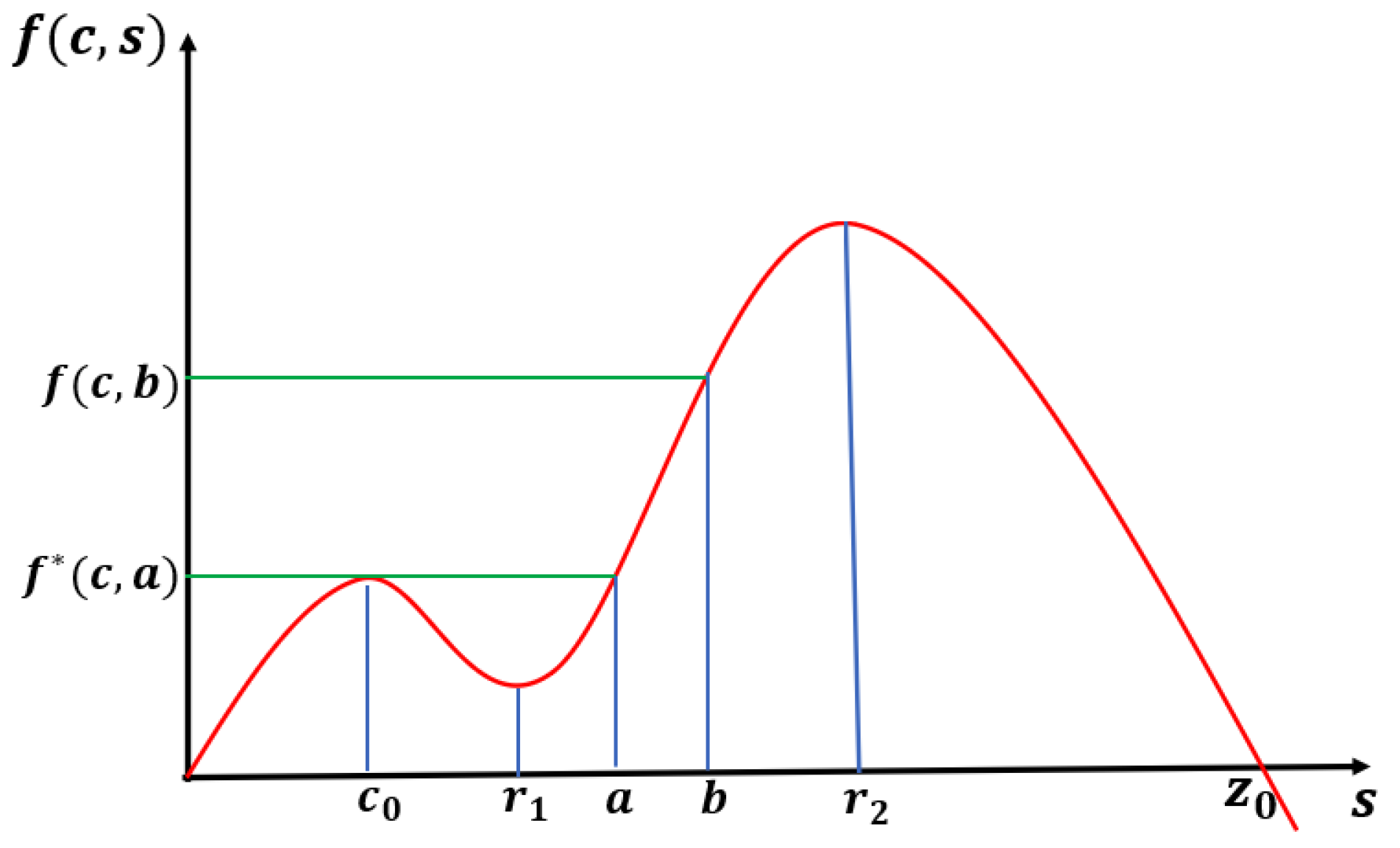
Proof of Theorem 5. 

Recall the subsolution ${\psi }_1:={\delta }_1{\tilde{\varphi }}_1$ for $\lambda >E_1(M,g_0(\mu ,c),\gamma )$ (here, $M=1$), strict subsolution ${\psi }_4$ for $\lambda \in \left({\displaystyle \frac{2bN{C}_N}{R^{2}f(c,b)}},{\displaystyle \frac{2r_{2}N}{f(c,b)R^2}}\right)$, supersolution $Z_1$ for $\lambda >0,$ and strict supersolution $Z_4={\displaystyle \frac{av(\mu ,b,c)}{{\parallel v(\mu ,b,c)\parallel }_{\infty }}}$ for $\lambda \in \left({\displaystyle \frac{2bN{C}_N}{R^{2}f(c,b)}},{\displaystyle \frac{a}{{\parallel v(\mu ,b,c)\parallel }_{\infty }{f}^{*}(c,a)}}\right).$ Since $a<z_0$, we have $Z_4<Z_1.$ By construction, we have $\parallel {\psi }_4{\parallel }_{\infty }>b>a={\parallel Z_4\parallel }_{\infty }.$ Choosing ${\delta }_1\approx 0$, we have ${\psi }_1\le {\psi }_4\le Z_1$. Then, by Lemma 2, the result follows. □

Justification of the Remark 3:

Here, we prove that our growth term f and emigration term g satisfy the conditions in Theorem 5 when $N=1,2,3$, and $\Omega$ is a ball of radius R.

Recall that $f(c,s)=s(1-s)-{\displaystyle \frac{c{s}^2}{m+s^2}}$. For simplicity of demonstration, we let $c=0.019,m=0.0001$. Note that

$$f^{\prime }(c,s)={\displaystyle \frac{2c{s}^3}{{(m+s^2)}^2}}-2s\left(1+{\displaystyle \frac{c}{m+s^2}}\right)+1=1-2s-{\displaystyle \frac{2mcs}{{(m+s^2)}^2}}$$

and $f^{\prime }(c,s)=0$ has three positive solutions $s=c_0,r_1$, and $r_2$ such that $c_0<r_1<r_2$ (see Figure 25). It can be shown that $c_0\approx 0.0032, r_1\approx 0.0097$, and $r_2\approx 0.5$. Note that $f(c,s)$ increases on $(0,c_0)\cup (r_1,r_2)$ and decreases on $(c_0,r_1)\cup (r_2,\infty )$ with respect to s. Hence $f(c,c_0)$ and $f(c,r_2)$ are the local maximum and $f(c,r_1)$ is a local minimum.

Figure 25. The shape of f along with the values of $c_0,a,b,r_1$, and $r_2$.

We choose $a=0.01454$ such that $f(c,a)=f(c,c_0)=f^{*}(c,a)$, and ${\displaystyle \frac{a}{f^{*}(c,a)}}\approx 10.1690$. Now, we will show that $b<{\displaystyle \frac{r_2}{C_N}}$ which will imply ${\displaystyle \frac{2N{C}_{N}b}{R^{2}f(c,b)}}<{\displaystyle \frac{2N{r}_2}{R^{2}f(c,b)}}$ for $N=1,2,3$. By choosing $b=0.1054$, we have $b<{\displaystyle \frac{r_2}{C_3}}\approx 0.1055$. This implies that $b<{\displaystyle \frac{r_2}{C_N}}$ for $N=1,2,3$ since $C_N$ is an increasing function of N. Then, we have

$$\begin{array}{c}\hfill {\displaystyle \frac{C_{3}b}{f(c,b)}}\approx 6.6217<{\displaystyle \frac{a}{f^{*}(c,a)}}\approx 10.1690\end{array}$$

(20)

We note that the solution $v(\mu ,b,c)$ of (5) is given by

$$v(\mu ,b,c)={\displaystyle \frac{R^2-{\left|x\right|}^2}{2N}}+{\displaystyle \frac{1}{\gamma g_{\infty }}}{\displaystyle \frac{R}{N}}\sqrt{{\displaystyle \frac{f(c,b)}{b}}{\displaystyle \frac{R^2}{2N{C}_N}}},$$

and ${\parallel v(\mu ,b,c)\parallel }_{\infty }\to {\displaystyle \frac{R^2}{2N}}$ as $\mu \to \infty$ since $g_{\infty }\ge \mu c\to \infty$ as $\mu \to \infty$. Hence, we have

$${\displaystyle \frac{2N{C}_{N}b}{R^{2}f(c,b)}}\le {\displaystyle \frac{2N}{R^2}}{\displaystyle \frac{C_{3}b}{f(c,b)}}<{\displaystyle \frac{2N}{R^2}}·{\displaystyle \frac{a}{f^{*}(c,a)}}={\displaystyle \frac{a}{\frac{R^2}{2N}{f}^{*}(c,a)}}$$

by (20) for $N=1,2,3$. Hence, when $\mu$ is large, we have

$${\displaystyle \frac{2N{C}_{N}b}{R^{2}f(c,b)}}<{\displaystyle \frac{a}{{\parallel v(\mu ,b,c)\parallel }_{\infty }{f}^{*}(c,a)}}.$$

Thus, we have ${\displaystyle \frac{2N{C}_{N}b}{R^{2}f(c,b)}}<min\left\{{\displaystyle \frac{a}{{\parallel v(\mu ,b,c)\parallel }_{\infty }{f}^{*}(c,a)}},{\displaystyle \frac{2N{r}_2}{R^{2}f(c,b)}}\right\}$ when $\mu$ is large for $N=1,2,3$.

We note that the principal eigenvalue $E_1^D$ (of (4)) when $\Omega$ is a ball of radius R is given by

$$E_1^D=\left\{\begin{array}{cc}{\displaystyle \frac{{\pi }^2}{4R^2}}\approx {\displaystyle \frac{2.4674}{R^2}}\hfill & N=1\hfill \\ {\displaystyle \frac{j_{0,1}^2}{R^2}}\approx {\displaystyle \frac{5.7832}{R^2}}\hfill & N=2\hfill \\ {\displaystyle \frac{j_{N/2-1,1}}{R^2}}<{\displaystyle \frac{\sqrt{N/2}(\sqrt{N/2+1}+1)}{R^2}}\hfill & N\ge 3\hfill \end{array}\right.$$

where $j_{n,1}$ is the first zero of the Bessel function of order n. From [33], we have $j_{n,1}<\sqrt{n+1}(\sqrt{n+2}+1)$ for $n>-1$, and $E_1^D<{\displaystyle \frac{\sqrt{N/2}(\sqrt{N/2+1}+1)}{R^2}}={\displaystyle \frac{\sqrt{1.5}(\sqrt{2.5}+1)}{R^2}}\approx {\displaystyle \frac{3.1612}{R^2}}$ when $N=3$. Then, $E_1^D<{\displaystyle \frac{6}{R^2}}$ and

$$E_1^D<{\displaystyle \frac{6}{R^2}}<{\displaystyle \frac{13.2520}{R^2}}={\displaystyle \frac{2r_2}{f(c,b)R^2}}\le {\displaystyle \frac{2N{r}_2}{f(c,b)R^2}}$$

for $N=1,2,3$. On the other hand, we have

$$E_1^D<{\displaystyle \frac{6}{R^2}}<{\displaystyle \frac{2\times 10.1690}{R^2}}={\displaystyle \frac{2a}{R^2{f}^{*}(c,a)}}\le {\displaystyle \frac{2Na}{R^2{f}^{*}(c,a)}}={\displaystyle \frac{a}{\frac{R^2}{2N}{f}^{*}(c,a)}}$$

This implies that $E_1(1,g_0(\mu ,c),\gamma )<E_1^D<{\displaystyle \frac{a}{{\parallel v(\mu ,b,c)\parallel }_{\infty }{f}^{*}(c,a)}}$ when $\mu$ is large for $N=1,2,3$ since ${\parallel v(\mu ,b,c)\parallel }_{\infty }\to {\displaystyle \frac{R^2}{2N}}$ as $\mu \to \infty$. Thus, we have $E_1(1,g_0(\mu ,c),\gamma )<min\left\{{\displaystyle \frac{a}{{\parallel v(\mu ,b,c)\parallel }_{\infty }{f}^{*}(c,a)}},{\displaystyle \frac{2N{r}_2}{R^{2}f(c,b)}}\right\}$ and

$$max\left\{E_1(1,g_0(\mu ,c),\gamma ),{\displaystyle \frac{2N{C}_{N}b}{R^{2}f(c,b)}}\right\}<min\left\{{\displaystyle \frac{a}{{\parallel v(\mu ,b,c)\parallel }_{\infty }{f}^{*}(c,a)}},{\displaystyle \frac{2N{r}_2}{R^{2}f(c,b)}}\right\}$$

holds when $N=1,2,3$. This completes the justification.

Proof of Theorem 6. 

Here, we prove the non-existence of a positive solution for $\lambda <E_1(1,g_0(\mu ,c),\gamma ).$

Note that $f(c,s)<s$ for all $s\in (0,\infty )$. Let ${\sigma }_0(1,g_0(\mu ,c),\lambda ,\gamma )$ be the principal eigenvalue and ${\varphi }_0>0;\overline{\Omega }$ be the corresponding normalized eigenfunction of (11). We note that ${\sigma }_0(1,g_0(\mu ,c),\lambda ,\gamma )>0$ when $\lambda <E_1(1,g_0(\mu ,c),\gamma )$ (see Lemma 4). Suppose $u_{\lambda }$ is a positive solution of (1) for $\lambda <E_1(1,g_0(\mu ,c),\gamma )$. Then, by Green’s Second Identity, we have

$$\begin{array}{ccc}\hfill {\int }_{\Omega }\left({\varphi }_0\Delta u_{\lambda }-u_{\lambda }\Delta {\varphi }_0\right)dx& =& {\int }_{\partial \Omega }\left({\varphi }_0{\displaystyle \frac{\partial u_{\lambda }}{\partial \eta }}-u_{\lambda }{\displaystyle \frac{\partial {\varphi }_0}{\partial \eta }}\right)ds\hfill \\ & =& {\int }_{\partial \Omega }\left(-{\varphi }_0\gamma \sqrt{\lambda }g(c,u_{\lambda })u_{\lambda }+\gamma u_{\lambda }\sqrt{\lambda }{g}_0(\mu ,c){\varphi }_0\right)ds\hfill \\ & =& {\int }_{\partial \Omega }\gamma {\varphi }_0{u}_{\lambda }\sqrt{\lambda }\left(g_0(\mu ,c)-g(c,u_{\lambda })\right)ds\hfill \\ & \le & 0.\hfill \end{array}$$

On the other hand, we have

$$\begin{array}{ccc}\hfill {\int }_{\Omega }\left({\varphi }_0\Delta u_{\lambda }-u_{\lambda }\Delta {\varphi }_0\right)dx& =& {\int }_{\Omega }\left(-{\varphi }_0\lambda f(c,u_{\lambda })+(\lambda +{\sigma }_0(1,g_0(\mu ,c),\lambda ,\gamma ))u_{\lambda }{\varphi }_0\right)dx\hfill \\ & >& {\int }_{\Omega }\left(-{\varphi }_0\lambda u_{\lambda }+(\lambda +{\sigma }_0(1,g_0(\mu ,c),\lambda ,\gamma ))u_{\lambda }{\varphi }_0\right)dx\hfill \\ & =& {\int }_{\Omega }{\sigma }_0(1,g_0(\mu ,c),\lambda ,\gamma ){\varphi }_0{u}_{\lambda }dx\hfill \\ & >& 0\hfill \end{array}$$

since $f(c,u_{\lambda })<u_{\lambda }$ and ${\sigma }_0(1,g_0(\mu ,c),\lambda ,\gamma )>0$ for $\lambda <E_1(1,g_0(\mu ,c),\gamma )$. This is a contradiction. Thus, (1) has no positive solution for $\lambda <E_1(1,g_0(\mu ,c),\gamma )$. □

Proof of Remark 3. 

Here, we prove non-existence for $\lambda <E_1(1,g_{\infty }\left(c\right),\gamma )$ in the Cases A and B. Recall that ${\sigma }_0={\sigma }_0(1,g_{\infty }\left(c\right),\gamma )>0$ for $\lambda <E_1(1,g_{\infty }\left(c\right),\gamma )$. Assume $u_{\lambda }$ is a positive solution of (1) for $\lambda <E_1(1,g_{\infty }\left(c\right),\gamma )$. Then, by Green’s Second Identity, we have

$$\begin{array}{cc}& {\int }_{\Omega }\left({\varphi }_0\Delta u_{\lambda }-u_{\lambda }\Delta {\varphi }_0\right)dx\hfill \\ \hfill & ={\int }_{\partial \Omega }\left({\varphi }_0{\displaystyle \frac{\partial u_{\lambda }}{\partial \eta }}-u_{\lambda }{\displaystyle \frac{\partial {\varphi }_0}{\partial \eta }}\right)ds\hfill \\ \hfill & ={\int }_{\partial \Omega }\left(-{\varphi }_0\sqrt{\lambda }\gamma g(c,u_{\lambda })u_{\lambda }+u_{\lambda }\sqrt{\lambda }\gamma g_{\infty }\left(c\right){\varphi }_0\right)ds\hfill \\ \hfill & ={\int }_{\partial \Omega }\gamma {\varphi }_0{u}_{\lambda }\sqrt{\lambda }\left(g_{\infty }\left(c\right)-g(c,u_{\lambda })\right)ds\hfill \\ \hfill & \le 0\hfill \end{array}$$

(21)

since $g(c,s)\ge g_{\infty }\left(c\right);[0,z_0]$. On the other hand, we have

$$\begin{array}{cc}& {\int }_{\Omega }\left({\varphi }_0\Delta u_{\lambda }-u_{\lambda }\Delta {\varphi }_0\right)dx\hfill \\ \hfill & ={\int }_{\Omega }\left(-{\varphi }_0\lambda f(c,u_{\lambda })+(\lambda +{\sigma }_0)u_{\lambda }{\varphi }_0\right)dx\hfill \\ \hfill & \ge {\int }_{\Omega }\left(-{\varphi }_0\lambda u_{\lambda }+(\lambda +{\sigma }_0)u_{\lambda }{\varphi }_0\right)dx\sin \mathrm{ce}f(c,u_{\lambda })\le u_{\lambda }\hfill \\ \hfill & ={\int }_{\Omega }{\varphi }_0{u}_{\lambda }\left(-\lambda +\lambda +{\sigma }_0\right)dx\hfill \\ \hfill & ={\int }_{\Omega }{\sigma }_0{\varphi }_0{u}_{\lambda }dx\hfill \\ \hfill & >0\sin \mathrm{ce}{\sigma }_0>0\mathrm{for}\lambda <E_1(1,g_{\infty }\left(c\right),\gamma ).\hfill \end{array}$$

(22)

This is a contradiction. Thus, (1) has no positive solution for $\lambda <E_1(1,g_{\infty }\left(c\right),\gamma )$. This completes the proof. □

Appendix A.1. Proof of Lemma 3

Let $u\left(x\right)$ be a positive solution of (7) such that $u\left(0\right)=u\left(1\right)=q$ and ${\parallel u\parallel }_{\infty }=\rho$. Multiplying both sides of (7) by $u^{\prime }$, we obtain

$$-u^{″}{u}^{\prime }=\lambda f(c,u)u^{\prime }.$$

Integrating both sides gives us

$$-{\displaystyle \frac{{\left(u^{\prime }\right)}^2}{2}}=\lambda F(c,u)+C.$$

Now using the fact that $u^{\prime }\left({\displaystyle \frac{1}{2}}\right)=\rho$, we obtain

$$u^{\prime }\left(x\right)=\sqrt[]{2\lambda \left[F\right(c,\rho )-F(c,u\left)\right]};\left[0,{\displaystyle \frac{1}{2}}\right)$$

(A1)

and

$$u^{\prime }\left(x\right)=-\sqrt[]{2\lambda \left[F\right(c,\rho )-F(c,u\left)\right]};\left({\displaystyle \frac{1}{2}},1\right].$$

(A2)

Since the solution is symmetric about $x={\displaystyle \frac{1}{2}}$, it is enough to consider the case $u^{\prime }\left(x\right)=\sqrt{2\lambda \left[F\right(c,\rho )-F(c,u\left)\right]}$ when $0<x<{\displaystyle \frac{1}{2}}$. Then, integrating both sides, we obtain

$${\int }_0^x{\displaystyle \frac{u^{\prime }\left(s\right)}{\sqrt[]{F(c,\rho )-F\left(u\right(s\left)\right)}}}ds=\sqrt{2\lambda }x;\left[0,{\displaystyle \frac{1}{2}}\right).$$

Using the substitution $z=u\left(s\right)$, we have

$${\int }_q^{u\left(x\right)}{\displaystyle \frac{ds}{\sqrt[]{F(c,\rho )-F(c,s)}}}=\sqrt{2\lambda }x;\left[0,{\displaystyle \frac{1}{2}}\right).$$

(A3)

By letting $x\to {\displaystyle \frac{1}{2}}$, we obtain

$${\int }_q^{\rho }{\displaystyle \frac{ds}{\sqrt[]{F(c,\rho )-F(c,s)}}}={\displaystyle \frac{\sqrt{2\lambda }}{2}};\left[0,{\displaystyle \frac{1}{2}}\right).$$

This implies that

$$\lambda =2{\left({\int }_{q\left(\rho \right)}^{\rho }{\displaystyle \frac{ds}{\sqrt[]{F(c,\rho )-F(c,s)}}}\right)}^2.$$

(A4)

Now, from (A1) and the boundary condition $-u^{\prime }\left(0\right)+\gamma \sqrt{\lambda }g(c,u\left(0\right))u\left(0\right)=0$ with $u\left(0\right)=q$, we obtain

$$-\sqrt{2\lambda \left[F\right(c,\rho )-F(c,q\left)\right]}+\gamma \sqrt{\lambda }g(c,q)q=0$$

which is equivalent to

$$2[F(c,\rho )-F(c,q)]={\gamma }^2{\left(g(c,q)\right)}^2{q}^2.$$

Conversely, assume that $\lambda ,\rho$ satisfy the equations

$$\lambda =2{\left({\int }_{q\left(\rho \right)}^{\rho }{\displaystyle \frac{ds}{\sqrt[]{F(c,\rho )-F(c,s)}}}\right)}^2$$

(A5)

and

$$2[F(c,\rho )-F(c,q)]={\gamma }^2{\left(g(c,q)\right)}^2{q}^2.$$

(A6)

Define $u:[0,1]\to [q,\rho ]$ by

$$\begin{array}{ccc}\hfill {\int }_q^{u\left(x\right)}{\displaystyle \frac{dz}{\sqrt{F(c,\rho )-F(c,z)}}}& =& \sqrt{2\lambda }x;x\in \left[0,{\displaystyle \frac{1}{2}}\right)\hfill \end{array}$$

(A7)

$$\begin{array}{ccc}\hfill {\int }_{\rho }^{u\left(x\right)}{\displaystyle \frac{dz}{\sqrt{F(c,\rho )-F(c,z)}}}& =& -\sqrt{2\lambda }\left(x-{\displaystyle \frac{1}{2}}\right);x\in \left({\displaystyle \frac{1}{2}},1\right]\hfill \end{array}$$

(A8)

and $u\left({\displaystyle \frac{1}{2}}\right)=\rho$.

We will now show that $u\left(x\right)$ is a positive solution of (7). The function

$$\begin{array}{c}\hfill {\displaystyle \frac{1}{\sqrt{2\lambda }}}{\int }_q^u{\displaystyle \frac{dz}{\sqrt{F(c,\rho )-F(c,z)}}},\end{array}$$

is a differentiable function of u which is strictly increasing from 0 to ${\displaystyle \frac{1}{2}}$ as u increases from q to $\rho$. Thus, for each $x\in [0,{\displaystyle \frac{1}{2}})$, there is a unique $u\left(x\right)$ such that

$$\begin{array}{ccc}\hfill {\int }_q^{u\left(x\right)}{\displaystyle \frac{dt}{\sqrt{F(c,\rho )-F(c,t)}}}& =& \sqrt{2\lambda }x.\hfill \end{array}$$

(A9)

Moreover, by the Implicit Function Theorem, $u\left(x\right)$ is differentiable with respect to x. Differentiating (A9) gives

$$\begin{array}{ccc}\hfill u^{\prime }\left(x\right)& =& \sqrt{2\left[F\right(c,\rho )-F(c,u\left(x\right)\left)\right]};x\in \left[0,{\displaystyle \frac{1}{2}}\right).\hfill \end{array}$$

(A10)

Through a similar argument, $u\left(x\right)$ is a differentiable, decreasing function of x for $x\in \left({\displaystyle \frac{1}{2}},1\right]$ with

$$\begin{array}{ccc}\hfill u^{\prime }\left(x\right)& =& -\sqrt{2\left[F\right(c,\rho )-F(c,u\left(x\right)\left)\right]};x\in \left({\displaystyle \frac{1}{2}},1\right].\hfill \end{array}$$

(A11)

These imply

$$\begin{array}{ccc}\hfill {\displaystyle \frac{{\left[u^{\prime }\left(x\right)\right]}^2}{2}}& =& F(c,\rho )-F(c,u(x\left)\right);x\in (0,1).\hfill \end{array}$$

Differentiating again, we have

$$\begin{array}{c}\hfill -u^{″}\left(x\right)=f(c,u\left(x\right));x\in (0,1).\end{array}$$

Thus, $u\left(x\right)$ satisfies Equation (7). Now, we show that $u\left(x\right)$ satisfies the boundary conditions in (7). Since q is a solution of (A6), we have

$$\begin{array}{c}\hfill F(c,\rho )-F(c,q)={\displaystyle \frac{{\gamma }^2{\left(g(c,q)\right)}^2{q}^2}{2}}.\end{array}$$

(A12)

Substituting $x=0$ into (A10) gives

$$\begin{array}{c}\hfill u^{\prime }\left(0\right)=\sqrt{2\lambda }\sqrt{F(c,\rho )-F(c,q)}.\end{array}$$

(A13)

Combining (A12) and (A13), we have

$$\begin{array}{c}\hfill -u^{\prime }\left(0\right)+\gamma \sqrt{\lambda }g(c,q)q=0.\end{array}$$

A similar argument shows that

$$\begin{array}{c}\hfill u^{\prime }\left(1\right)+\gamma \sqrt{\lambda }g(c,q)q=0.\end{array}$$

Hence, $u\left(x\right)$ satisfies (7), and the proof is complete.