On the Construction of a Two-Step Sixth-Order Scheme to Find the Drazin Generalized Inverse

Abstract

This study introduces a numerically efficient iterative solver for computing the Drazin generalized inverse, addressing a critical need for high-performance methods in matrix computations. The proposed two-step scheme achieves sixth-order convergence, distinguishing it as a higher-order method that outperforms several existing approaches. A rigorous convergence analysis is provided, highlighting the importance of selecting an appropriate initial value to ensure robustness. Extensive numerical experiments validate the analytical findings, showcasing the method’s superior speed and efficiency, making it an advancement in iterative solvers for generalized inverses.

1. Preliminary Remarks

The computation of generalized inverses remains an area of significant research in computational mathematics (see, for example, [1,2]). Over the past 63 years, substantial advancements have been achieved in this field. Early contributions by E.H. In 1920, Moore pioneered the concept of a generalized algebraic matrix inverse, yet the field gained momentum only after 1955, as marked by the works of Penrose (1955, 1956), Golub and Kahan (1965), and Rao and Mitra (1971) as discussed in [3]. These and other significant contributions have defined much of the field, establishing foundations that allow limited scope for new developments [4].

Terms such as “the pseudo-inverse”, “{2}-inverse”, and “the minimum-norm least squares inverse” are widely utilized, often more so than “Drazin inverse”, to denote unique matrix inverses in applications involving the resolution of linear systems and optimization [5].

Greville’s foundational partitioning approach in computing generalized inverses was examined in [3]. While effective, this solver incurs a high operational cost and greater round-off errors. Many numerical solvers devised for the Drazin generalized inverse often lack computational stability, prompting the need to explore and propose new iterative approaches that address these limitations; see the discussions in [6] for more.

In numerical computation, it is essential to counteract cumulative rounding errors effectively; symbolic computation achieves this by preserving variable precision throughout the process. However, the symbolic computation of the Drazin inverse becomes computationally intensive for matrices of high dimensionality, which has led investigators to propose computationally effective iteration solvers methods for this target [7,8].

The general solution for a square singular linear system of the form

$$\mathrm{\Gamma }y=\varphi ,$$

(1)

can be expressed as

$$y={\mathrm{\Gamma }}^D\varphi +(I-\mathrm{\Gamma }{\mathrm{\Gamma }}^D)z,$$

(2)

utilizing the Drazin generalized inverse, whereas z$\in \mathcal{N}\left(\mathrm{\Gamma }\right)+\mathcal{R}\left({\mathrm{\Gamma }}^{\iota -1}\right)$, as investigated in [9]. For example, in control theory, the Drazin inverse helps to determine the solution of descriptor systems, which are characterized by differential–algebraic equations. These systems often model engineering processes involving constraints, such as electrical circuits with dependent components or robotic mechanisms with non-holonomic constraints. The Drazin inverse ensures that solutions respect the system’s algebraic constraints, providing stability and robustness in the analysis.

We describe ${\mathbb{C}}^{N\times N}$ and ${\mathbb{C}}_r^{N\times N}$ as the sets of $N\times N$ square matrices with complex entries and those of rank r, in the respective order. Additionally, $\mathrm{\Gamma }$, $\mathcal{N}\left(\mathrm{\Gamma }\right)$, $\mathrm{rank}\left(\mathrm{\Gamma }\right)$, and $\mathcal{R}\left(\mathrm{\Gamma }\right)$ represent the conjugate transpose, null space, rank, and range of $\mathrm{\Gamma }\in {\mathbb{C}}^{N\times N}$.

Drazin introduced a generalized inverse, non-reflexive yet commuting with elements of associative rings and semigroups, in his seminal paper [10]. Wilkinson further elaborated on its significance and computation in [11]. The study of the Drazin inverse spans multiple domains, including matrix theory (specifically within generalized inverses) and ring theory.

A dynamical system governed by a homogeneous equation is referred to as pointwise complete if every possible terminal state of the system can be attained by appropriately selecting its initial state. Conversely, a system that fails to exhibit this property is described as pointwise degenerate. The concepts of pointwise completeness and degeneracy have been extensively studied in various contexts, including linear continuous-time systems with delays, as well as fractional linear discrete-time systems, as highlighted in the literature [12]. Furthermore, the Drazin inverse of matrices has proven to be a valuable tool for analyzing the pointwise completeness and degeneracy of descriptor fractional linear systems.

In recent years, significant advancements have been made in extending these mathematical notions. The author of [13] has generalized the concepts of the Drazin inverse, the Core–Moore–Penrose inverse, and the Drazin–Moore–Penrose inverse of finite square matrices to finite potent endomorphisms. This work has introduced numerous properties of these extended inverses, thereby broadening their applicability. Notably, all results derived for finite potent endomorphisms remain valid for the special case of finite square matrices, thereby enriching the theoretical framework and providing deeper insights into the structural characteristics of these systems.

The Drazin inverse is particularly useful in the computation of spectral projectors, which separate the behavior of a system into stable and unstable dynamics. This is essential for understanding and controlling dynamical systems in engineering fields like aerodynamics and robotics. It also has applications in network theory, where it aids in determining steady-state solutions in Markov chains with absorbing states, which is crucial for designing efficient communication or traffic flow systems.

To proceed, we first furnish some essential definitions [3].

Definition 1.

The minimum non-negative integer ι for which

$$rank\left({\mathrm{\Gamma }}^{\iota +1}\right)=rank\left({\mathrm{\Gamma }}^{\iota }\right),$$

(3)

holds is known as the index of Γ, represented by $ind\left(\mathrm{\Gamma }\right)$.

Definition 2.

Consider a complex matrix Γ of order $N\times N$. The Drazin inverse of Γ, shown via ${\mathrm{\Gamma }}^D$, is the distinct matrix Θ that fulfills the conditions below

$$\left(1\right){\mathrm{\Gamma }}^{\iota }\mathrm{\Theta }\mathrm{\Gamma }={\mathrm{\Gamma }}^{\iota },\left(2\right)\mathrm{\Theta }\mathrm{\Gamma }\mathrm{\Theta }=\mathrm{\Theta },\left(3\right)\mathrm{\Gamma }\mathrm{\Theta }=\mathrm{\Theta }\mathrm{\Gamma },$$

(4)

where $\iota =\mathrm{ind}\left(\mathrm{\Gamma }\right)$, the matrix index of Γ.

As long as $\mathrm{ind}\left(\mathrm{\Gamma }\right)=1$, $\mathrm{\Theta }$ is termed the group inverse of $\mathrm{\Gamma }$. For nonsingular $\mathrm{\Gamma }$, $\mathrm{ind}\left(\mathrm{\Gamma }\right)=0$, yielding ${\mathrm{\Gamma }}^D={\mathrm{\Gamma }}^{-1}$.

The idempotent matrix $\mathrm{\Gamma }{\mathrm{\Gamma }}^D$ serves as a projector onto $\mathcal{R}\left({\mathrm{\Gamma }}^{\iota }\right)$ along $\mathcal{N}\left({\mathrm{\Gamma }}^{\iota }\right)$, where $\mathcal{R}\left({\mathrm{\Gamma }}^{\iota }\right)$ is the range of ${\mathrm{\Gamma }}^{\iota }$ and $\mathcal{N}\left({\mathrm{\Gamma }}^{\iota }\right)$ its null space. For nilpotent $\mathrm{\Gamma }$, ${\mathrm{\Gamma }}^D=0$; see [14] for further details.

Matrix iteration schemes are sensitive to the selection of the starting value ${\mathrm{\Theta }}_0$ for convergence towards ${\mathrm{\Gamma }}^D$. Iteration solvers such as Schulz-like schemes are especially efficient for sparse matrices with sparse inverses, though often hampered by the need for an appropriate initial guess. The literature provides numerous approaches to this initial selection, as discussed comprehensively in [15].

To highlight key innovations of the proposed method compared to existing methods, in this article, we provide the following:

• Introduction of an iterative approach for computing the Drazin inverse.
• Improvement in CPU time compared to well-known existing methods.
• Analytical investigation of the method’s behavior.
• Superior computational efficiency due to reduced computational complexity.

Following this introduction in this section, the rest of the work is structured as follows:

• Section 2 reviews key iteration solvers for the inverse of Drazin.
• In Section 3, we present our novel high-order scheme. Section 4 examines its sixth-order convergence characteristics.
• Section 5 addresses the computational complexity of iterative schemes, identifying the optimal choice.
• Section 6 applies our new scheme to illustrate reduced CPU time.
• Section 7 presents the final observations and insights.

2. Associated Studies

A classic approach for computing the inverse of an invertible $\mathrm{\Gamma }$ is the Schulz scheme, presented in [16], as comes next:

$${\mathrm{\Theta }}_{\varpi +1}={\mathrm{\Theta }}_{\varpi }(2I-\mathrm{\Gamma }{\mathrm{\Theta }}_{\varpi }),\varpi =0,1,2,\dots ,$$

(5)

where I denotes the unit matrix with identical dimensions to $\mathrm{\Gamma }$.

The authors of [17] extended the applicability of the Schulz method (5) by proving its effectiveness to calculate the Drazin inverse for square matrices. They introduced the starting value below:

$${\mathrm{\Theta }}_0=\alpha {\mathrm{\Gamma }}^l,l\ge \mathrm{ind}\left(\mathrm{\Gamma }\right)=\iota ,$$

(6)

wherein $\alpha$ is selected such that we have

$$\parallel I-\mathrm{\Gamma }{\mathrm{\Theta }}_0\parallel <1.$$

(7)

Utilizing an initial guess as (6) in conjunction with (5) yields a quadratically convergent iteration process for computing the inverse of Drazin.

Next, we review several higher-order iterative methods for this purpose, recognizing that efficiency gains are essential since the Schulz method (5) converges slowly in the early iteration stages, thereby increasing the overall computational effort required for matrix inversion.

The authors of [18] proposed an iteration scheme with a cubic convergence rate, formulated as

$${\mathrm{\Theta }}_{\varpi +1}={\mathrm{\Theta }}_{\varpi }(3I-\mathrm{\Gamma }{\mathrm{\Theta }}_{\varpi }(3I-\mathrm{\Gamma }{\mathrm{\Theta }}_{\varpi })),\varpi =0,1,2,\dots ,$$

(8)

alongside an alternative scheme of the same order for approximating ${\mathrm{\Gamma }}^{-1}$ (or ${\mathrm{\Gamma }}^D$ with a suitable initial choice), defined by

$${\mathrm{\Theta }}_{\varpi +1}={\mathrm{\Theta }}_{\varpi }\left[{\displaystyle \frac{1}{2}}(I-\mathrm{\Gamma }{\mathrm{\Theta }}_{\varpi })(I+{(2I-\mathrm{\Gamma }{\mathrm{\Theta }}_{\varpi })}^2)+I\right],\varpi =0,1,2,\dots .$$

(9)

Additionally, a generalized approach to derive similar iteration sequences is outlined in [19] (Chapter 5). The authors provided a 4th-order solver as follows:

$${\mathrm{\Theta }}_{\varpi +1}={\mathrm{\Theta }}_{\varpi }(I+{\mathrm{\Xi }}_{\varpi }(I+{\mathrm{\Xi }}_{\varpi }(I+{\mathrm{\Xi }}_{\varpi }))),\varpi =0,1,2,\dots ,$$

(10)

where ${\mathrm{\Xi }}_{\varpi }=I-\mathrm{\Gamma }{\mathrm{\Theta }}_{\varpi }$. More broadly, by applying Schröder’s generalized iterative method [20] to the nonlinear problem

$$\mathrm{\Gamma }\mathrm{\Theta }=I,$$

(11)

we can derive the following solver [21]:

$$\begin{array}{ccc}{\mathrm{\Theta }}_{\varpi +1}\hfill & =\hfill & {\mathrm{\Theta }}_{\varpi }(I+{\mathrm{\Xi }}_{\varpi }+{\mathrm{\Xi }}_{\varpi }^2+\cdots +{\mathrm{\Xi }}_{\varpi }^{m-1})\hfill \\ \hfill & =\hfill & {\mathrm{\Theta }}_{\varpi }(I+{\mathrm{\Xi }}_{\varpi }(I+{\mathrm{\Xi }}_{\varpi }(\cdots +{\mathrm{\Xi }}_{\varpi })\dots )),\varpi =0,1,2,\dots ,\hfill \end{array}$$

(12)

with convergence order m, which requires m Horner-like matrix multiplications, where ${\mathrm{\Xi }}_{\varpi }=I-\mathrm{\Gamma }{\mathrm{\Theta }}_{\varpi }$.

Recently, the authors of [5], through additional factorization and simplification steps, proposed the following iterative scheme:

$${\mathrm{\Theta }}_{\varpi +1}={\mathrm{\Theta }}_{\varpi }\left(I+{\mathrm{\Xi }}_{\varpi }\right)\left[(I+{\beta }_1{\mathrm{\Xi }}_{\varpi }^2+{\mathrm{\Xi }}_{\varpi }^4)(I+{\beta }_2{\mathrm{\Xi }}_{\varpi }^2+{\mathrm{\Xi }}_{\varpi }^4)\right],$$

(13)

which reduces the computational load to only six matrix–matrix multiplications per cycle. Here, the constants ${\beta }_1$ and ${\beta }_2$ are given by

$${\beta }_1={\displaystyle \frac{1}{2}}\left(1-\sqrt{5}\right),{\beta }_2={\displaystyle \frac{1}{2}}\left(1+\sqrt{5}\right).$$

(14)

3. Development of a Novel Iterative Approach

The impetus for this manuscript is to develop a multi-step rapid iterative solver that enhances both accuracy and efficiency in addressing nonlinear equations; see the pioneer discussions in the works [22,23]. By avoiding the necessity for second Fréchet derivatives, our approach seeks to mitigate the complexities and computational overhead associated with existing methodologies.

An iterative family of Chebyshev–Halley methods was first introduced and studied by [24,25], designed to locate simple roots of the following nonlinear problem:

$$g\left(x\right)=0,$$

which can be presented as follows:

$$x_{\varpi +1}=x_{\varpi }-\left(1+{\displaystyle \frac{1}{2}}{\displaystyle \frac{L\left(x_{\varpi }\right)}{1-aL\left(x_{\varpi }\right)}}\right){\displaystyle \frac{g\left(x_{\varpi }\right)}{g^{\prime }\left(x_{\varpi }\right)}},$$

(15)

wherein $a\in \mathbb{R}$,

$$L\left(x_{\varpi }\right)={\displaystyle \frac{g^{″}\left(x_{\varpi }\right)g\left(x_{\varpi }\right)}{g^{\prime }{\left(x_{\varpi }\right)}^2}},$$

and the convergence order is cubic; for recent discussions about the solutions of nonlinear equations, see [26,27,28]. This scheme is an extension of the famous Newton’s solver [29], which is given by

$$x_{\varpi +1}=x_{\varpi }-{\displaystyle \frac{g\left(x_{\varpi }\right)}{g^{\prime }\left(x_{\varpi }\right)}},$$

(16)

Here, we need to resolve the nonlinear problem below:

$$X^{-1}=A.$$

(17)

In the scalar version of (17), we obtain Schulz and Chebyshev’s methods as discussed in Section 2. To propose a two-step method, we combine these two solvers by using

$$\begin{array}{c}\hfill \left\{\begin{array}{c}{y}_{\varpi }=x_{\varpi }-\left(1+{\displaystyle \frac{1}{2}}{\displaystyle \frac{g^{″}\left(x_{\varpi }\right)g\left(x_{\varpi }\right)}{g^{\prime }{\left(x_{\varpi }\right)}^2}}\right){\displaystyle \frac{g\left(x_{\varpi }\right)}{g^{\prime }\left(x_{\varpi }\right)}},\hfill \\ x_{\varpi +1}=y_{\varpi }-{\displaystyle \frac{g\left(y_{\varpi }\right)}{g^{\prime }\left(y_{\varpi }\right)}}.\hfill \end{array}\right.\end{array}$$

(18)

Note that for Chebyshev’s method, involved in the first step of (18), its convergence for nonlinear equations was studied in [30]. To enhance the efficiency of this approach, we apply a series of factorization steps to streamline the expression in (18) to solve (17), thereby decreasing the matrix–matrix products involved. This yields

$$\begin{array}{c}\hfill \left\{\begin{array}{c}{\mathrm{\Lambda }}_{\varpi }={\mathrm{\Theta }}_{\varpi }(3I-\mathrm{\Gamma }{\mathrm{\Theta }}_{\varpi }(3I-\mathrm{\Gamma }{\mathrm{\Theta }}_{\varpi })),\hfill \\ {\mathrm{\Theta }}_{\varpi +1}={\mathrm{\Lambda }}_{\varpi }(2I-\mathrm{\Gamma }{\mathrm{\Lambda }}_{\varpi }),\hfill \end{array}\right.\end{array}$$

(19)

which requires five matrix–matrix products per iteration.

Schulz-type iterations, as exemplified in (19), are inherently numerically stable, exhibiting a self-correcting property and based primarily on efficient matrix multiplications per cycle as long as a proper initial guess is used. This framework is well suited to parallel processing, particularly with sparse matrices. Integrating (19) with sparse-saving techniques can further alleviate the computational demands of matrix–matrix products within each cycle.

The scheme in (19) for calculating the Drazin inverse converges, provided that the initial approximation is selected as [31]

$${\mathrm{\Theta }}_0={\displaystyle \frac{2}{\mathrm{Tr}\left({\mathrm{\Gamma }}^{\iota +1}\right)}}{\mathrm{\Gamma }}^{\iota },$$

(20)

or equivalently,

$${\mathrm{\Theta }}_0={\displaystyle \frac{1}{{2\parallel \mathrm{\Gamma }\parallel }_2^{\iota +1}}}{\mathrm{\Gamma }}^{\iota },$$

(21)

where $\mathrm{Tr}(·)$ denotes the trace of a matrix under $\iota$.

An examination of the convergence behavior of this solver is provided in the next section, and we offer detailed insights into the selection of an initial approximation that maintains the iteration convergence rate. Additionally, we outline conditions under which this novel approach may be effectively applied to compute the Drazin inverse of square matrices.

Before presenting the primary theorems concerning the convergence analysis and convergence speed of the furnished solver, we first outline several key lemmas.

Proposition 1

([31]). Consider $\mathrm{\Gamma }\in {\mathbb{C}}^{N\times N}$ and a given $\epsilon >0$. A norm $\parallel ·\parallel$ is identified for which

$$\rho \left(\mathrm{\Gamma }\right)+ϵ\ge \parallel \mathrm{\Gamma }\parallel \ge \rho \left(\mathrm{\Gamma }\right),$$

(22)

where $\rho \left(\mathrm{\Gamma }\right)$ represents the spectral radius of Γ, defined as the maximum absolute value of its eigenvalues.

Proposition 2

([31]). Let $P_{L,M}$ denote the projection onto a subspace L along a subspace M. Next,

(i) $P_{L,M}Q=Q$ iff $\mathcal{R}\left(Q\right)\subseteq L$;

(ii) $Q{P}_{L,M}=Q$ iff $\mathcal{N}\left(Q\right)\supseteq M$.

4. Theoretical Parts

Theorem A0.

Suppose that $\mathrm{\Gamma }\in {\mathbb{C}}^{N\times N}$ is an invertible matrix. Additionally, suppose the starting matrix ${\mathrm{\Theta }}_0$ is chosen according to either (6) or (20) and (21). Consequently, the sequence of matrices ${\left\{{\mathrm{\Theta }}_{\varpi }\right\}}_{\varpi =0}^{\infty }$ generated by (19) adheres to the following error bound for approximating the Drazin inverse:

$${\displaystyle \frac{\parallel {\mathrm{\Gamma }}^D-{\mathrm{\Theta }}_{\varpi }\parallel }{\parallel {\mathrm{\Gamma }}^D\parallel }}\le {\parallel I-\mathrm{\Gamma }{\mathrm{\Theta }}_0\parallel }^{6^{\varpi }}.$$

(23)

Moreover, the convergence rate of the method is six.

Proof. 

We proceed by considering

$$\begin{array}{ll}{\mathrm{\Xi }}_{\varpi +1}& =I-\mathrm{\Gamma }{\mathrm{\Theta }}_{\varpi +1}\\ & =I-\mathrm{\Gamma }\left({\mathrm{\Lambda }}_{\varpi }(2I-\mathrm{\Gamma }{\mathrm{\Lambda }}_{\varpi })\right)\\ & =I-\mathrm{\Gamma }\left(\left({\mathrm{\Theta }}_{\varpi }(3I-\mathrm{\Gamma }{\mathrm{\Theta }}_{\varpi }(3I-\mathrm{\Gamma }{\mathrm{\Theta }}_{\varpi }))\right)\right(2I\\ & -\mathrm{\Gamma }\left({\mathrm{\Theta }}_{\varpi }(3I-\mathrm{\Gamma }{\mathrm{\Theta }}_{\varpi }(3I-\mathrm{\Gamma }{\mathrm{\Theta }}_{\varpi }))\right)\left)\right)\\ & ={(I-\mathrm{\Gamma }{\mathrm{\Theta }}_{\varpi })}^6\\ & ={\mathrm{\Xi }}_{\varpi }^6.\end{array}$$

(24)

By applying an arbitrary matrix norm to the expression in (24), one can rewrite it as follows:

$$\parallel {\mathrm{\Xi }}_{\varpi +1}\parallel \le \parallel {\mathrm{\Xi }}_{\varpi }{\parallel }^6.$$

(25)

Given that ${\mathrm{\Theta }}_0$ is selected according to either (6) or (20) and (21), it subsequently follows that

$$\mathrm{\Xi }\left({\mathrm{\Theta }}_0\right)\subseteq \mathrm{\Xi }\left({\mathrm{\Gamma }}^{\iota }\right).$$

(26)

This can now be expressed as

$$\mathrm{\Xi }\left({\mathrm{\Theta }}_{\varpi }\right)\subseteq \mathrm{\Xi }\left({\mathrm{\Theta }}_{\varpi -1}\right).$$

(27)

It is now concluded that

$$\mathrm{\Xi }\left({\mathrm{\Theta }}_{\varpi }\right)\subseteq \mathrm{\Xi }\left({\mathrm{\Gamma }}^{\iota }\right),\varpi \ge 0.$$

(28)

In a similar fashion, if the proposed solver for computing the Drazin inverse is formulated by performing left multiplication on ${\mathrm{\Theta }}_{\varpi }$, it can be concluded that

$$\mathcal{N}\left({\mathrm{\Theta }}_{\varpi }\right)\supseteq \mathcal{N}\left({\mathrm{\Gamma }}^{\iota }\right),\varpi \ge 0.$$

(29)

At this point, by applying the definition of the Drazin inverse, one obtains

$$\mathrm{\Gamma }{\mathrm{\Gamma }}^D={\mathrm{\Gamma }}^D\mathrm{\Gamma }=P_{\mathcal{R}\left({\mathrm{\Gamma }}^{\iota }\right),\mathcal{N}\left({\mathrm{\Gamma }}^{\iota }\right)}.$$

(30)

By combining Proposition 2 with the expressions in (28)–(30), it follows that

$${\mathrm{\Theta }}_{\varpi }\mathrm{\Gamma }{\mathrm{\Gamma }}^D={\mathrm{\Theta }}_{\varpi }={\mathrm{\Gamma }}^D\mathrm{\Gamma }{\mathrm{\Theta }}_{\varpi },\varpi \ge 0.$$

(31)

In order to finalize the proof, we continue as outlined below. The matrix representing the error is given by ${\delta }_{\varpi }={\mathrm{\Gamma }}^D-{\mathrm{\Theta }}_{\varpi }$ satisfies the following

$$\begin{array}{ll}{\delta }_{\varpi }& ={\mathrm{\Gamma }}^D-{\mathrm{\Theta }}_{\varpi }\\ & ={\mathrm{\Gamma }}^D-{\mathrm{\Gamma }}^D\mathrm{\Gamma }{\mathrm{\Theta }}_{\varpi }\\ & ={\mathrm{\Gamma }}^D\left(I-\mathrm{\Gamma }{\mathrm{\Theta }}_{\varpi }\right)\\ & ={\mathrm{\Gamma }}^D{\mathrm{\Xi }}_{\varpi }.\end{array}$$

Utilizing (25), one attains

$$\parallel {\delta }_{\varpi }\parallel =\parallel {\mathrm{\Gamma }}^D\parallel \parallel {\mathrm{\Xi }}_{\varpi }\parallel \le \parallel {\mathrm{\Gamma }}^D\parallel \parallel {\mathrm{\Xi }}_0{\parallel }^{6^{\varpi }}.$$

(32)

This serves as a verification of the result in (23). As an immediate consequence of (32) and Proposition 2, it follows that we can derive

$$\begin{array}{ll}\mathrm{\Gamma }{\delta }_{\varpi +1}& =\mathrm{\Gamma }{\mathrm{\Gamma }}^D-\mathrm{\Gamma }{\mathrm{\Theta }}_{\varpi +1}\\ & =\mathrm{\Gamma }{\mathrm{\Gamma }}^D-I+I-\mathrm{\Gamma }{\mathrm{\Theta }}_{\varpi +1}\\ & =\mathrm{\Gamma }{\mathrm{\Gamma }}^D-I+{\mathrm{\Xi }}_{\varpi +1}.\end{array}$$

(33)

By examining (24) and performing a series of simplifications, we arrive at the conclusion that

$$\mathrm{\Gamma }{\delta }_{\varpi +1}=\mathrm{\Gamma }{\mathrm{\Gamma }}^D-I+{\mathrm{\Xi }}_{\varpi }^6.$$

(34)

Utilizing the idempotent characteristic ${(I-\mathrm{\Gamma }{\mathrm{\Gamma }}^D)}^t=(I-\mathrm{\Gamma }{\mathrm{\Gamma }}^D)$, where $t\ge 1$ denotes a natural number, along with the subsequent result derived from (31), we obtain the following:

$$\begin{array}{ll}(I-\mathrm{\Gamma }{\mathrm{\Gamma }}^D)\mathrm{\Gamma }{\delta }_{\varpi }& =(I-\mathrm{\Gamma }{\mathrm{\Gamma }}^D)\mathrm{\Gamma }({\mathrm{\Gamma }}^D-{\mathrm{\Theta }}_{\varpi })\\ & ={\mathrm{\Theta }}_{\varpi }-\mathrm{\Gamma }{\mathrm{\Gamma }}^D{\mathrm{\Theta }}_{\varpi }\\ & =0.\end{array}$$

(35)

As a result, for every $t\ge 1$, we arrive at the following expression (where we apply (35) during the simplification process):

$$\begin{array}{ll}{\left({\mathrm{\Xi }}_{\varpi }\right)}^t+\mathrm{\Gamma }{\mathrm{\Gamma }}^D-I& ={(I-\mathrm{\Gamma }{\mathrm{\Theta }}_{\varpi })}^t+\mathrm{\Gamma }{\mathrm{\Gamma }}^D-I\\ & ={(I-\mathrm{\Gamma }{\mathrm{\Gamma }}^D+\mathrm{\Gamma }{\mathrm{\Gamma }}^D-\mathrm{\Gamma }{\mathrm{\Theta }}_{\varpi })}^t+\mathrm{\Gamma }{\mathrm{\Gamma }}^D-I\\ & ={\left((I-\mathrm{\Gamma }{\mathrm{\Gamma }}^D)+\mathrm{\Gamma }{\delta }_{\varpi }\right)}^t+\mathrm{\Gamma }{\mathrm{\Gamma }}^D-I\\ & =I-\mathrm{\Gamma }{\mathrm{\Gamma }}^D+{\left(\mathrm{\Gamma }{\delta }_{\varpi }\right)}^t+\mathrm{\Gamma }{\mathrm{\Gamma }}^D-I\\ & ={\left(\mathrm{\Gamma }{\delta }_{\varpi }\right)}^t.\end{array}$$

(36)

By combining (34) and (36), it follows that

$$\mathrm{\Gamma }{\delta }_{\varpi +1}={\left(\mathrm{\Gamma }{\delta }_{\varpi }\right)}^6.$$

(37)

Finally, one obtains

$$\parallel \mathrm{\Gamma }{\delta }_{\varpi +1}\parallel \le \parallel \mathrm{\Gamma }{\delta }_{\varpi }{\parallel }^6.$$

(38)

At this point, it becomes evident how to determine the error bound for the proposed iterative scheme (19), by taking into account (38) along with the second criterion outlined in (4), which pertains to the computation of the Drazin inverse, as demonstrated below:

$$\begin{array}{ll}\parallel {\delta }_{\varpi +1}\parallel & =\parallel {\mathrm{\Theta }}_{\varpi +1}-{\mathrm{\Gamma }}^D\parallel \\ & =\parallel {\mathrm{\Gamma }}^{D}A{V}_{\varpi +1}-{\mathrm{\Gamma }}^D\mathrm{\Gamma }{\mathrm{\Gamma }}^D\parallel \\ & =\parallel {\mathrm{\Gamma }}^D(\mathrm{\Gamma }{\mathrm{\Theta }}_{\varpi +1}-\mathrm{\Gamma }{\mathrm{\Gamma }}^D)\parallel \\ & \le \parallel {\mathrm{\Gamma }}^D\parallel \parallel \mathrm{\Gamma }{\delta }_{\varpi +1}\parallel \\ & \le {\parallel {\mathrm{\Gamma }}^D\parallel \parallel {\delta }_{\varpi }\parallel }^6.\end{array}$$

(39)

The inequalities presented in (39) lead to the conclusion that ${\mathrm{\Theta }}_{\varpi }$ converges to ${\mathrm{\Gamma }}^D$ as $\varpi \to +\infty$, with a convergence rate of the sixth order. We consider summarizing key points for readers unfamiliar with iterative methods as follows:

• The convergence proof demonstrates that the error decreases exponentially, with a sixth-order convergence rate, ensuring rapid approximation of the Drazin inverse.
• A key feature is the reduction in computational effort due to fewer matrix–matrix multiplications while maintaining high accuracy.
• The choice of an appropriate initial value plays a crucial role in ensuring the method’s reliability.
• These insights provide a clear understanding of why the proposed method outperforms existing iterative schemes in both speed and efficiency, especially when the matrix norm-2 is required for each computing step.

This completes the proof.    □

5. Efficiency Comparison

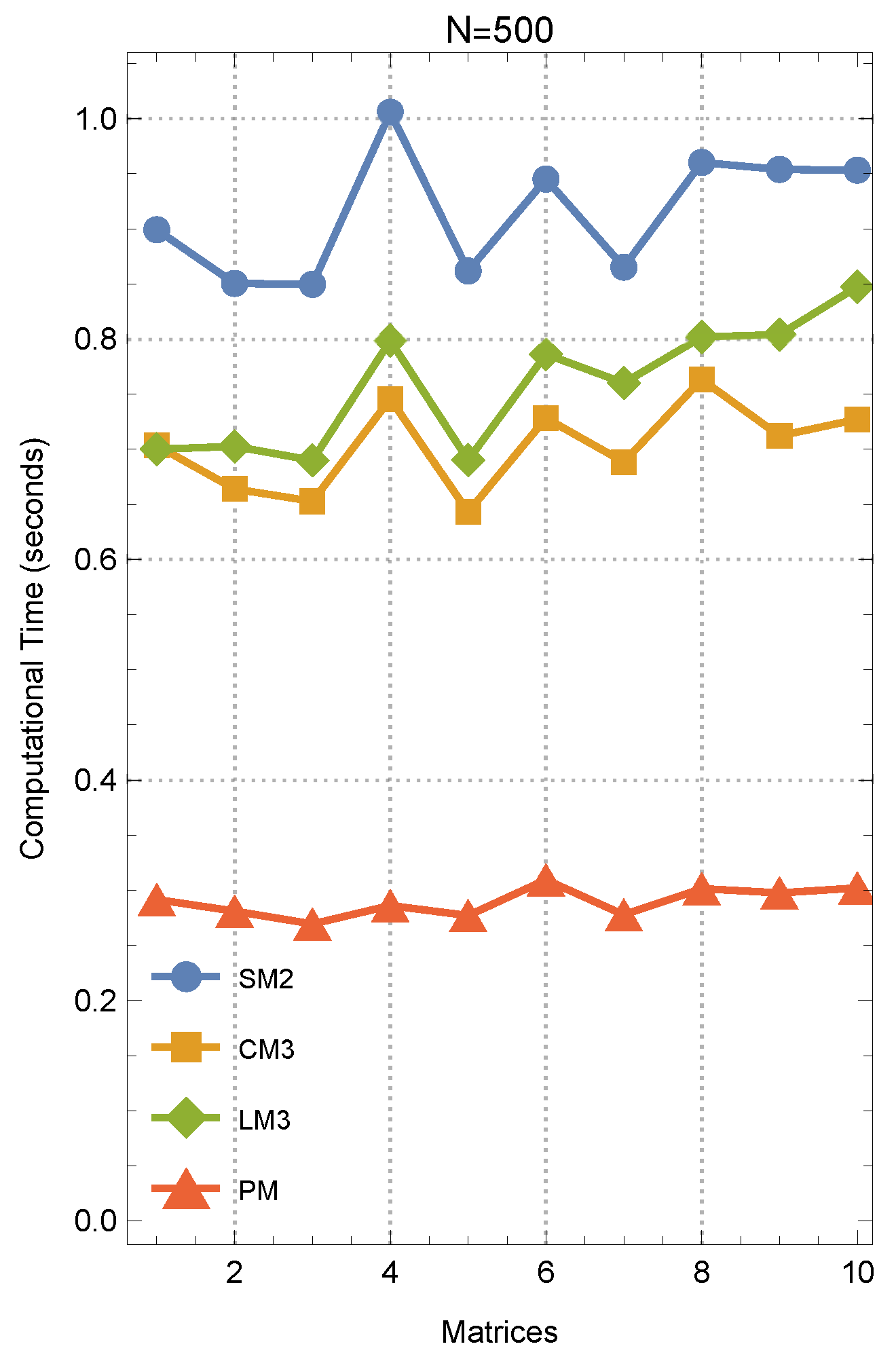
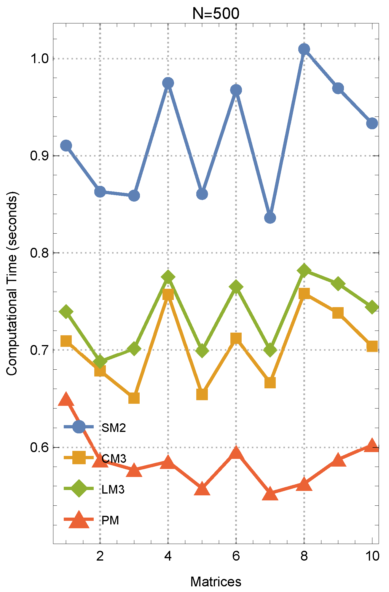
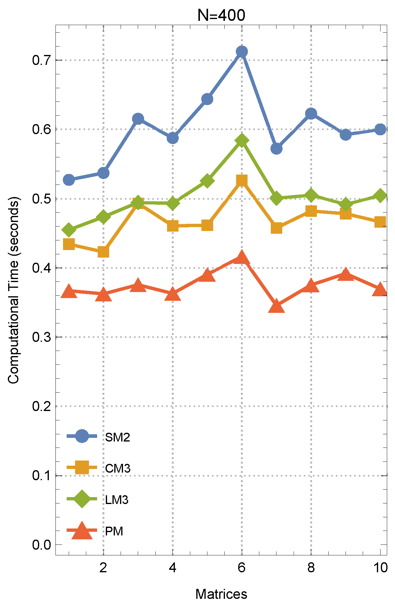
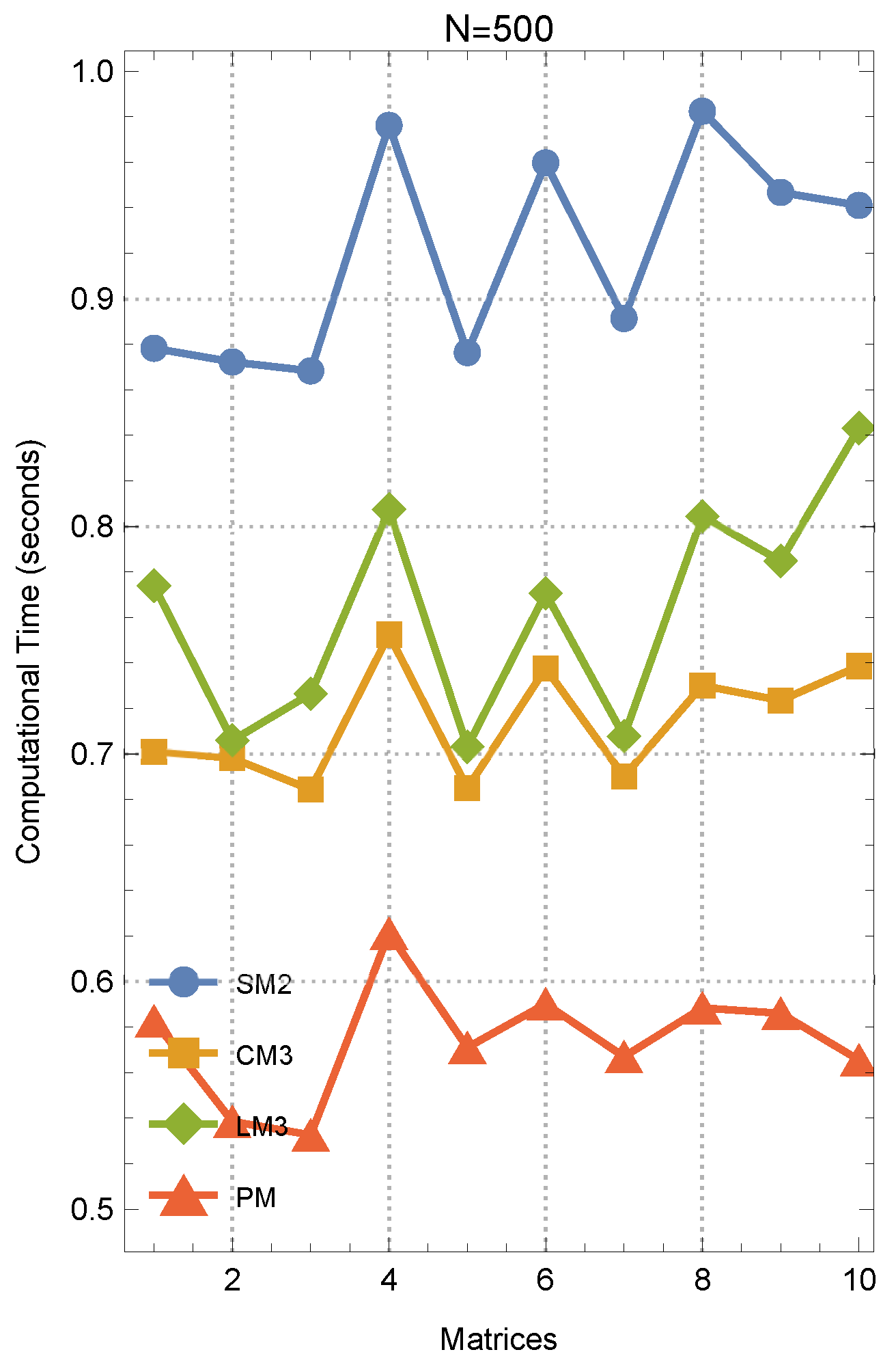
As discussed earlier, an effective iterative method is distinguished by its high convergence rate paired with minimal computational cost. When finding the Drazin inverse, a significant portion of computational resources is often consumed by matrix products.

Assuming unit cost for each matrix–matrix product, as is typical in floating-point calculations, we recall the inverse-finder informational efficiency index (IEI). It utilizes $\rho$ and $\kappa$, representing the convergence rate and the quantity of matrix–matrix multiplications, in the respective order, and is defined as follows [20]:

$$IEI={\displaystyle \frac{\rho }{\kappa }}.$$

(40)

On the other hand, the efficiency index (EI) for iterative solvers is defined as follows [20]:

$$EI=\sqrt[\kappa ]{\rho },$$

(41)

where $\kappa$ represents the total computational cost. Thus, we undertake a theoretical analysis to compare the computational efficiency of various iterative schemes—namely, (5), (8), (9), (10), and (19)—as each of these approaches can converge to ${\mathrm{\Gamma }}^D$ provided a suitable initial guess is selected (6). An analytically favorable scheme should, therefore, aim to achieve a high convergence speed $\rho$ with a minimal quantity of matrix–matrix products $\kappa$ relative to competing methods, ideally satisfying $\kappa \le \rho$.

The results summarized in Table 1 demonstrate that, for various values of $\upsilon$, the EIs of PM1 and PM2 outperform those of their competitors. The results confirm the almost equal or superior performance and enhanced efficiency of PM methods when compared to the main competing methods.

Table 1. A comparative analysis of the computational load associated with various methods, each evaluated across various indices.

Solvers	(5)	(8)	(9)	(10)	(19)
$\rho$	2	3	3	4	6
$\kappa$	2	3	4	4	5
IEI	${\displaystyle \frac{2}{2}}=1$	${\displaystyle \frac{3}{3}}=1$	${\displaystyle \frac{3}{4}}=0.75$	${\displaystyle \frac{4}{4}}=1$	${\displaystyle \frac{6}{5}}\approx 1.2$
EI	$2^{\frac{1}{2}}\simeq 1.41$	$3^{\frac{1}{3}}\simeq 1.44$	$3^{\frac{1}{4}}\simeq 1.31$	$4^{\frac{1}{4}}\simeq 1.41$	$6^{\frac{1}{5}}\simeq 1.43$

6. Experiments

This section examines the computational precision and efficiency in calculating the Drazin inverse. The proposed iterative scheme (19) is notable for its implementation without requiring matrix exponentiation, facilitating its straightforward application in computing generalized inverses. For comparative computational analysis, we employ the schemes (5), (8), (9), and (19), referenced as SM2, CM3, LM3, and PM, in the respective order.

Several points merit attention:

• Simulations are conducted using Mathematica 13.0 [32,33].
• Computation times for obtaining approximate inverses are measured in seconds.
• When reporting elapsed times, all methods under comparison are executed within an identical computational environment.

Experiment 1.

This test is conducted to compute the Drazin inverse, given that the matrix is specified as in [17]:

$$\mathrm{\Gamma }=\left[\begin{array}{cccccccccccc}2& 4/10& 0& 0& 0& 0& 0& 0& 0& 0& 0& 0\\ -2& 4/10& 0& 0& 0& 0& 0& 0& 0& 0& 0& 0\\ -1& -1& 1& -1& 0& 0& 0& 0& -1& 0& 0& 0\\ -1& -1& -1& 1& 0& 0& 0& 0& 0& 0& 0& 0\\ 0& 0& 0& 0& 1& 1& -1& -1& 0& 0& -1& 0\\ 0& 0& 0& 0& 1& 1& -1& -1& 0& 0& 0& 0\\ 0& 0& 0& -1& -2& 4/10& 0& 0& 0& 0& 0& 0\\ 0& 0& 0& 0& 2& 4/10& 0& 0& 0& 0& 0& 0\\ 0& -1& 0& 0& 0& 0& 0& 0& 1& -1& -1& -1\\ 0& 0& 0& 0& 0& 0& 0& 0& -1& 1& -1& -1\\ 0& 0& 0& 0& 0& 0& 0& 0& 0& 0& 4/10& -2\\ 0& 0& 0& 0& 0& 0& 0& 0& 0& 0& 4/10& 2\end{array}\right],$$

with $\iota =\mathrm{ind}\left(\mathrm{\Gamma }\right)=3$. The Drazin inverse in its exact form can be expressed as

$${\mathrm{\Gamma }}^D=\left[\begin{array}{cccccccccccc}0.25& -0.25& 0.& 0.& 0.& 0.& 0.& 0.& 0.& 0.& 0.& 0.\\ 1.25& 1.25& 0.& 0.& 0.& 0.& 0.& 0.& 0.& 0.& 0.& 0.\\ -1.66& -0.99& 0.25& -0.25& 0.& 0.& 0.& 0.& -0.06& -0.06& 0.& 0.15\\ -1.19& -0.67& -0.25& 0.25& 0.& 0.& 0.& 0.& -0.06& 0.18& 0.68& 1.34\\ -2.76& -1.04& -1.87& -1.25& -1.25& 1.25& 1.25& 1.25& 1.48& 2.57& 3.32& 6.64\\ -2.76& -1.04& -1.87& -1.25& -1.25& 1.25& 1.25& 1.25& 1.48& 2.57& 4.57& 8.51\\ 14.10& 6.30& 6.62& 3.37& 5.& -3.& -5.& -5.& -4.18& -8.5& -10.50& -22.46\\ -19.32& -8.50& -9.75& -5.25& -7.5& 4.5& 7.5& 7.5& 6.37& 12.56& 15.97& 33.78\\ -0.62& -0.31& 0.& 0.& 0.& 0.& 0.& 0.& 0.25& -0.25& -0.87& -1.62\\ -1.25& -0.93& 0.& 0.& 0.& 0.& 0.& 0.& -0.25& 0.25& -0.87& -1.62\\ 0.& 0.& 0.& 0.& 0.& 0.& 0.& 0.& 0.& 0.& 1.25& 1.25\\ 0.& 0.& 0.& 0.& 0.& 0.& 0.& 0.& 0.& 0.& -0.25& 0.25\end{array}\right].$$

The termination criterion is defined as $\parallel {\mathrm{\Theta }}_{\iota +1}-{\mathrm{\Theta }}_{\iota }{\parallel }_{\infty }\le {10}^{-6}$. Verifying the requirements outlined in Definition 2 for the proposed iterative method PM leads to

$$\begin{gathered} \parallel {\mathrm{\Gamma }}^{\iota +1}{\mathrm{\Gamma }}^D-{\mathrm{\Gamma }}^{\iota }{\parallel }_{\infty }=2.58\times {10}^{-11}, \\ \parallel {\mathrm{\Gamma }}^D\mathrm{\Gamma }{\mathrm{\Gamma }}^D-{\mathrm{\Gamma }}^D{\parallel }_{\infty }=4.87\times {10}^{-11}, \\ {\parallel \mathrm{\Gamma }{\mathrm{\Gamma }}^D-{\mathrm{\Gamma }}^D\mathrm{\Gamma }\parallel }_{\infty }=7.64\times {10}^{-9}, \end{gathered}$$

(42)

which provides validation for the theoretical analysis.

Experiment 2.

The purpose of this test is to evaluate and compare the CPU times taken by various solvers when applied to ten randomly generated square matrices (denoted here by A for simplicity in coding) using the following piece of code:

• ClearAll["Global‘*"]
• SeedRandom[12];
• n1 = 500; n2 = n1; number = 10; max1 = 75;
• Table[A[j] = RandomReal[{0, 1}, {n1, n2}], {j, number}];
• In this test, convergence is determined by the stopping criterion $\parallel {\mathrm{\Theta }}_{\varpi +1}-{\mathrm{\Theta }}_{\varpi }{\parallel }_2\le {10}^{-6}$. Additionally, the initial value is generated by means of

  $${\mathrm{\Theta }}_0={\displaystyle \frac{{\mathrm{\Gamma }}^T}{{\left|\right|\mathrm{\Gamma }\left|\right|}_2^2}}.$$

The outcomes of the comparative analysis for this test are displayed in Figure 1 and Figure 2 (for two different choices of input size), where computations for regular inverses were carried out with a standard precision of 15 digits. Evidently, higher-order methods necessitate fewer iterations for convergence; hence, the primary emphasis is placed on the computational time required to achieve the specified tolerance. It can be observed that our proposed scheme (19) outperforms its competitors, further validating the theoretical discussions in Section 3.

Figure 1. A comparative analysis of CPU times for different solvers, as conducted for Experiment 2, is presented for matrices of size $400\times 400$.

Figure 2. A comparison of the CPU times for different solvers for Experiment 2 for matrices of size $500\times 500$.

Experiment 3.

The objective of this test is to evaluate and compare the CPU times required by various solvers under the conditions of Experiment 2, modifying only the stopping criteria: $\parallel {\mathrm{\Theta }}_{\varpi +1}-{\mathrm{\Theta }}_{\varpi }{\parallel }_2\le {10}^{-4}$ and ${\parallel {\mathrm{\Theta }}_{\varpi +1}-{\mathrm{\Theta }}_{\varpi }\parallel }_2\le {10}^{-8}$.

The results of the comparative analysis are illustrated in Figure 3, Figure 4, Figure 5 and Figure 6, and they provide evidence supporting the effectiveness and robustness of the proposed two-step solver for computing (generalized) inverses. The numerical experiments demonstrate that the sixth-order convergence of our method outperforms traditional iterative approaches, particularly in terms of computational efficiency and in norm 2. Across all test cases, our method requires fewer iterations and exhibits faster computational times, even when subjected to diverse stopping criteria. Furthermore, the method demonstrates exceptional scalability, effectively handling matrices of varying dimensions, including those with randomly generated entries.

Figure 3. A comparison of the CPU times for different solvers for Experiment 3 for matrices of size $400\times 400$ when $\parallel {\mathrm{\Theta }}_{\varpi +1}-{\mathrm{\Theta }}_{\varpi }{\parallel }_2\le {10}^{-4}$.

Figure 4. A comparison of the CPU times for different solvers for Experiment 3 for matrices of size $500\times 500$ when $\parallel {\mathrm{\Theta }}_{\varpi +1}-{\mathrm{\Theta }}_{\varpi }{\parallel }_2\le {10}^{-4}$.

Figure 5. A comparison of the CPU times for different solvers for Experiment 3 for matrices of size $400\times 400$ when $\parallel {\mathrm{\Theta }}_{\varpi +1}-{\mathrm{\Theta }}_{\varpi }{\parallel }_2\le {10}^{-8}$.

Figure 6. A comparison of the CPU times for different solvers for Experiment 3 for matrices of size $500\times 500$ when $\parallel {\mathrm{\Theta }}_{\varpi +1}-{\mathrm{\Theta }}_{\varpi }{\parallel }_2\le {10}^{-8}$.

Additionally, the two-step iterative framework ensures that the solver remains computationally efficient under varying input configurations, which is critical for applications involving high-dimensional datasets. Moreover, the high order of convergence directly translates into reduced computational complexity, making the method particularly advantageous for resource-intensive scenarios. Unlike lower-order methods, which may struggle to balance speed and accuracy, our solver achieves a trade-off between these two metrics. This makes it an ideal choice for real-world applications requiring rapid solutions to generalized inverse problems.

7. Conclusions

The Drazin inverse is a fundamental concept in matrix theory, with its calculation being both challenging and highly applicable in practice. In conclusion, this study has presented a numerically efficient two-step iterative solver designed for calculating the Drazin generalized inverse with a sixth-order convergence rate, which qualifies it as a higher-order solver. We have rigorously analyzed the convergence properties of the proposed scheme, particularly emphasizing the importance of selecting an appropriate initial value, ${\mathrm{\Theta }}_0$, to ensure convergence towards ${\mathrm{\Gamma }}^D$.

Our findings have demonstrated that matrix iteration schemes are highly sensitive to this initial value selection, especially for sparse matrices. The proposed method builds upon traditional Schulz-like iteration schemes, addressing the challenges associated with requiring an optimal initial guess while providing enhanced computational efficiency.

Extensive numerical tests have confirmed the theoretical results, showcasing both the speed and effectiveness of the proposed solver. Moreover, our analysis has revealed that this novel iterative approach achieves substantial improvements in CPU time over existing methods by reducing the quantity of matrix–matrix products. The obtained results further validate the effectiveness of the proposed iterative method (19), demonstrated by a notable decrease in the elapsed CPU times. This efficiency makes our solver particularly suitable for applications requiring the Drazin inverse, contributing a significant advancement to iteration solvers in numerical linear algebra.

References

- Ghorbanzadeh, M.; Mahdiani, K.; Soleymani, F.; Lotfi, T. A class of Kung-Traub-Type iterative algorithms for matrix inversion. Int. J. Appl. Comput. Math. 2016, 2, 641–648. [Google Scholar] [CrossRef]
- Zehra, A.; Younus, A.; Tunç, C. Controllability and observability of linear impulsive differential algebraic system with Caputo fractional derivative. Comput. Methods Differ. Equ. 2022, 10, 200–214. [Google Scholar]
- Ben-Israel, A.; Greville, T.N.E. Generalized Inverses: Theory and Applications, 2nd ed.; Springer: New York, NY, USA, 2003. [Google Scholar]
- Ma, X.; Kumar Nashine, H.; Shil, S.; Soleymani, F. Exploiting higher computational efficiency index for computing outer generalized inverses. Appl. Numer. Math. 2022, 175, 18–28. [Google Scholar] [CrossRef]
- Jebreen, H.B.; Chalco-Cano, Y. An improved computationally efficient method for finding the Drazin inverse. Discrete Dyn. Nat. Soc. 2018, 2018, 6758302. [Google Scholar] [CrossRef]
- Guo, L.; Hu, G.; Yu, D.; Luan, T. A representation of the Drazin inverse for the sum of two matrices and the anti-triangular block matrices. Mathematics 2023, 11, 3661. [Google Scholar] [CrossRef]
- Sayevand, K.; Pourdarvish, A.; Machado, J.A.T.; Erfanifar, R. On the calculation of the Moore-Penrose and Drazin inverses: Application to fractional calculus. Mathematics 2021, 9, 2501. [Google Scholar] [CrossRef]
- Shil, S.; Kumar Nashine, H.; Soleymani, F. On an inversion-free algorithm for the nonlinear matrix problem . Int. J. Comput. Math. 2022, 99, 2555–2567. [Google Scholar] [CrossRef]
- Wei, Y. Index splitting for the Drazin inverse and the singular linear system. Appl. Math. Comput. 1998, 95, 115–124. [Google Scholar] [CrossRef]
- Drazin, M.P. Pseudoinverses in associative rings and semigroups. Amer. Math. Monthly 1958, 65, 506–514. [Google Scholar] [CrossRef]
- Wilkinson, J.H. Note on the practical significance of the Drazin inverse. In Recent Applications of Generalized Inverses, Pitman Advanced Publishing Program; Campbell, S.L., Ed.; Research Notes in Mathematics No. 66, Boston; Pitman: London, UK, 1982; pp. 82–99. [Google Scholar]
- Kaczorek, T.; Ruszewski, A. Application of the Drazin inverse to the analysis of pointwise completeness and pointwise degeneracy of descriptor fractional linear continuous-time systems. Int. J. Appl. Math. Comput. Sci. 2020, 30, 219–223. [Google Scholar] [CrossRef]
- Romo, F.P. On G-Drazin inverses of finite potent endomorphisms and arbitrary square matrices. Linear and Multilinear Algebra 2022, 70, 2227–2247. [Google Scholar] [CrossRef]
- Kyrchei, I. Explicit formulas for determinantal representations of the Drazin inverse solutions of some matrix and differential matrix equations. Appl. Math. Comput. 2013, 219, 7632–7644. [Google Scholar] [CrossRef]
- Pan, V.Y. Structured Matrices and Polynomials: Unified Superfast Algorithms; BirkhWauser: Boston, FL, USA; Springer: New York, NY, USA, 2001. [Google Scholar]
- Schulz, G. Iterative Berechnung der Reziproken matrix. Z. Angew. Math. Mech. 1933, 13, 57–59. [Google Scholar] [CrossRef]
- Li, X.; Wei, Y. Iterative methods for the Drazin inverse of a matrix with a complex spectrum. Appl. Math. Comput. 2004, 147, 855–862. [Google Scholar] [CrossRef]
- Li, H.-B.; Huang, T.-Z.; Zhang, Y.; Liu, X.-P.; Gu, T.-X. Chebyshev-type methods and preconditioning techniques. Appl. Math. Comput. 2011, 218, 260–270. [Google Scholar] [CrossRef]
- Krishnamurthy, E.V.; Sen, S.K. Numerical Algorithms—Computations in Science and Engineering; Affiliated East-West Press: New Delhi, India, 1986. [Google Scholar]
- Traub, J.F. Iterative Methods for Solution of Equations; Prentice-Hall: Englewood Cliffs, NJ, USA, 1964. [Google Scholar]
- Sen, S.K.; Prabhu, S.S. Optimal iterative schemes for computing Moore-Penrose matrix inverse. Int. J. Sys. Sci. 1976, 8, 748–753. [Google Scholar] [CrossRef]
- Bini, D.A. Numerical computation of the roots of Mandelbrot polynomials: An experimental analysis. Electron. Trans. Numer. Anal. 2024, 61, 1–27. [Google Scholar] [CrossRef]
- Ogbereyivwe, O.; Atajeromavwo, E.J.; Umar, S.S. Jarratt and Jarratt-variant families of iterative schemes for scalar and system of nonlinear equations. Iran. J. Numer. Anal. Optim. 2024, 14, 391–416. [Google Scholar]
- Hernández, M.; Salanova, M. A family of Chebyshev-Halley type methods. Int. J. Comput. Math. 1993, 47, 59–63. [Google Scholar] [CrossRef]
- Ivanov, S.I. Unified convergence analysis of Chebyshev-Halley methods for multiple polynomial zeros. Mathematics 2022, 10, 135. [Google Scholar] [CrossRef]
- Amat, S.; Busquier, S. After notes on Chebyshev’s iterative method. Appl. Math. Nonlinear Sci. 2017, 2, 1–12. [Google Scholar]
- Artidiello, S.; Cordero, A.; Torregrosa, J.R.P.; Vassileva, M. Generalized inverses estimations by means of iterative methods with memory. Mathematics 2020, 8, 2. [Google Scholar] [CrossRef]
- Torkashvand, V.; Kazemi, M.; Azimi, M. Efficient family of three-step with-memory methods and their dynamics. Comput. Methods Differ. Equ. 2024, 12, 599–609. [Google Scholar]
- Canela, J.; Evdoridou, V.; Garijo, A.; Jarque, X. On the basins of attraction of a one-dimensional family of root finding algorithms: From Newton to Traub. Math. Z. 2023, 303, 55. [Google Scholar] [CrossRef]
- Kostadinova, S.G.; Ivanov, S.I. Chebyshev’s method for multiple zeros of analytic functions: Convergence, dynamics and real-world applications. Mathematics 2024, 12, 3043. [Google Scholar] [CrossRef]
- Soleymani, F.; Stanimirović, P.S. A higher order iterative method for computing the Drazin inverse. Sci. World J. 2013, 2013, 708647. [Google Scholar] [CrossRef]
- Sánchez León, J.G. Mathematica Beyond Mathematics: The Wolfram Language in the Real World; Taylor & Francis Group: Boca Raton, FL, USA, 2017. [Google Scholar]
- Trott, M. The Mathematica Guide-Book for Numerics; Springer: New York, NY, USA, 2006. [Google Scholar]
Disclaimer/Publisher’s Note: The statements, opinions and data contained in all publications are solely those of the individual author(s) and contributor(s) and not of MDPI and/or the editor(s). MDPI and/or the editor(s) disclaim responsibility for any injury to people or property resulting from any ideas, methods, instructions or products referred to in the content. |
© 2024 by the authors. Licensee MDPI, Basel, Switzerland. This article is an open access article distributed under the terms and conditions of the Creative Commons Attribution (CC BY) license (https://creativecommons.org/licenses/by/4.0/).