Research on Change Point Detection during Periods of Sharp Fluctuations in Stock Prices–Based on Bayes Method β-ARCH Models

Abstract

In periods of dramatic stock price volatility, the identification of change points in stock price time series is important for analyzing the structural changes in financial market data, as well as for risk prevention and control in the financial market. As their residuals follow a generalized error distribution, the problem of estimating the change point parameters of the $\beta$-ARCH model is solved by combining the Kalman filtering method and the Bayes method innovatively, and we give a method for parameter estimation of the Bayes factors for the occurrences of change points, the expected values of the change point positions, and the variance of the change points. By detecting the change points of the price of eight stocks with a high number of limit up and limit down changes occurring in the observation period, the following conclusions are obtained: (1) Change point detection using the $\beta$-ARCH model based on the Bayes method is effective. (2) For different values of $\beta$, this research study finds that based on the classical ARCH model (i.e., $\beta =1$) of the change point parameter, the results are relatively optimal. (3) The accuracy of change point detection can be improved by correcting stock short-term effects by using the Kalman filtering method.

1. Introduction

In recent years, due to the acceleration of financial deleveraging and other policies, China’s stock markets have experienced many instances of volatility, which have brought large losses to investors and triggered economic turmoil. In this context, scientifically analyzing the structural changes in stock prices is crucial for investors’ investment decisions and regulators’ risk prevention and control.

With the widespread application of statistical inference theories and methods in the financial industry, more scholars have found that the study of change point problems has good predictive effects for identifying major events such as financial crises. Change points are actually qualitative changes in the data structure. It is very meaningful to accurately judge or predict the occurrences or locations of change points based on existing, historical, and all observable information [1].

When there is a significant fluctuation in the stock market, it is usually accompanied by limit up and limit down changes in individual stock prices. The price limits of the Chinese stock markets form a type of price stability mechanism, which is an institutional tool used by exchanges to control abnormal market fluctuations. They externally control trading prices within a certain range rather than as a natural result of price formation. Therefore, most scholars are concerned about how they affect the pricing efficiency of the market, i.e., whether there is a “cooling effect”, a “magnetic attraction effect”, or a “volatility spillover” [2,3,4], and few scholars have focused on their impact on the statistical characteristics of securities market prices. From the perspective of statistical inference, the impact of price limits on the market is short-term market friction formed by trading mechanisms on stock prices, which should not cause structural changes in price time series but may cause statistical bias. If this issue is ignored, there may be a certain degree of deviation in the estimation of the change point.

The statistical biases due to price limits in stock markets may originate from price latency problems. Price latency is the phenomenon of lagging price adjustments to traded assets under market friction. Previous studies have shown that low stock liquidity can lead to price delays, resulting in spurious auto-positive correlation in the index yield series and spurious auto-negative correlation in the time series of bases, which lead to statistical artifacts [3,5]. Harris pointed out that price limits can also lead to price latency problems [6]. In our preliminary work, we found that after correcting for the price distortion caused by price limits on CSI 500 Index components, the autocorrelation of index returns disappeared. Obviously, if the problem of statistical artifacts caused by price delays is ignored, the market may be misinterpreted; thus, wrong conclusions may be drawn. Therefore, during periods of significant market volatility, if the statistical biases caused by price limits can be corrected to some extent, this is expected to improve the accuracy of change point detection.

The study of statistical inference for change point problems started with Page [7] and has been a branch of research in statistics; it effectively integrates fixed sampling methods, successive sampling methods, hypothesis testing, statistical controls, Bayes methods, and other methods to solve the problems of change point occurrence and position estimation.

Based on their statistical methods, the existing studies can be divided into two categories. One category uses parameters and semi-parameters for change point testing and estimation; the other category uses the nonparametric testing and estimation of change points. For research on the change point problem in finance, due to the consensus in the academic community that ARCH models are suitable for analyzing financial market data, and the relatively low efficiency of nonparametric tests and their poor ability to detect differences, the estimation of change point parameters based on ARCH models has been widely adopted.

These studies achieve change point estimation based on the cumulative sums of residuals, likelihood functions, distribution functions, and Bayes methods. Among them, the studies presented by Kokoszka and Leipus [8,9], Lee et al. [10,11,12], Kim [13], and Andreou and Ghysels et al. [14] mainly constructed the cumulative sum of the residuals by the least squares method and used this statistic to estimate a solution to the change point problem based on the ARCH term parameters, mean, variance, and cross-covariance by using ARCH or GARCH models. In the study of estimating change points by using likelihood functions, it is common to construct statistics based on likelihood functions to identify the occurrence of change points. For example, Carsoule and Franses [15] proposed a sequential testing approach based on a maximum likelihood estimation method to solve the variance estimation problem and the ARCH model in the EUR exchange rate market. Berkes et al. [16] used a quasi-likelihood method to construct scoring statistics to solve the problem of change point estimation when using a GARCH model. Bardet and Kengne [17] proposed a change point estimation method suitable for a cluster of causal models (such as AR(∞), ARCH(∞), TARCH(∞), and ARMA-GARCH); the authors discussed a quasi-likelihood estimation index. In a study using distribution functions, Horvath and Kokoszka [18] derived the asymptotic distribution of a squared empirical residual term and applied it to the variation point detection problem by using an ARCH model. Na et al. [19] considered the problem of monitoring distribution change points for independent random sequences by using GARCH and other models by implementing an empirical distribution function model and empirical feature function type statistics. In the study of the change point problem using classical Bayes methods, parameter estimation is often carried out for models with relatively complex forms; e.g., Lai and Xing [20] studied the Bayesian change point parameter estimation problem by using an ARX-GARCH model. Wang et al. [21] proposed a quantile regression model with multiple random change points for a special panel to analyze the potential structural changes in the price capacity relationship after short-term stock issuances on the Chinese growth enterprise market. There are also some studies that focused on the detection of multivariate points in time-series models. Most of these studies transform multivariate point detection into a single-change point detection problem through binary segmentation. Representative studies include Fryzlewic and Rao [22], Cho and Fryzlewicz [23], etc.

In addition, since the Bayes method avoids the difficulty of finding a sampling distribution, it can also solve the problem of change point estimation through a general programming process under the condition of an abnormal prior assumption. Therefore, it has been widely applied in other fields. For example, Chen et al. [24] studied the identification of change points under the condition that climate change follows the Pareto distribution. Monfared, Dehghan and Fazlollah [25] studied change point identification under the assumption of a gamma distribution. Bianchi et al. [26] assumed that the volatility of macroeconomic risk exposure factors follows a breakpoint latent process and estimated the change point problem of risk factors. Jung, Song, and Chung [27] studied change point estimation under the condition of dynamic level distribution. Cai et al. [28] constructed a Bayes probability statistical inference model by using the Poisson distribution, the power-law distribution, and the log-normal distribution as prior distributions to test the change points of crude oil.

Through the above literature review, it is found that research on the estimation of change point parameters can be further supplemented in the following aspects: (1) The statistical bias caused by the price limits may be ignored. (2) Most existing studies only give research results on standard ARCH or GARCH models, while there is relatively little research on extended forms of ARCH models, such as the $\beta$-ARCH model. (3) The characteristics of the sharp peaks and heavy tails of financial asset prices lead to the fact that it is usually difficult to satisfy the assumption of normal distribution of model residuals, and Bayes change point detection using the generalized error distribution as a prior assumption is still rare.

Based on such a research status, this study is planned to be carried out along the following lines: First, in Section 2, a general extension form for the ARCH model, the $\beta$-ARCH model assuming that the residual follows a generalized error distribution, uses the classical Bayes methods to solve the parameter estimation problem of identifying the occurrence of change points and determining the position of change points. Then, in Section 3, by taking individual stocks with high frequency triggering the price limit in the Chinese stock market as an example, we use the Kalman filtering method to correct price distortions caused by price limits. Finally, in Section 4, the empirical test of change point detection is given, and the corresponding conclusions are obtained for the method proposed in this paper.

2. ARCH Model Change Point Detection

2.1. Introduction to the Model

In this paper, a nonlinear time-series model of the ARCH model is used to describe the time series of stock returns (see Equation (1)).

$$\left\{\begin{array}{c}{Y}_t={\epsilon }_t·h_t^{1/m}\\ h_t={\alpha }_0+{\alpha }_1{\left|Y_{t-1}\right|}^{m\beta }+\cdots +{\alpha }_q{\left|Y_{t-q}\right|}^{m\beta }\end{array}\right.$$

(1)

where $m>0,0<\beta \le 1$; ${\alpha }_0>0$, and ${\alpha }_i\ge 0$, with $i=1,\cdots ,q$. ${\epsilon }_t$, $t\ge 1$ are independently and identically distributed random variables (i.i.d.) and satisfy $E{\epsilon }_t=0E|{\epsilon }_t{|}^m=1$. In addition, we assume that $\left\{{\epsilon }_t\right\}$ is a “continuous density function that is positive everywhere”, which is independent of $\{Y_s,s<t\}$. When $m=2$, the model is called $\beta$-ARCH(q) model, as first proposed by Diebolt and Guégan [29]. When $m=2$ and $\beta =1$, the $\beta$-ARCH(q) model reduces to the classical ARCH(q) model, as proposed by Engle [30]. When modeling an ARCH model for a time series, it is usually assumed that the residual terms follow a normal distribution, a t-distribution, or a generalized error distribution (GED). Since the GED can flexibly account for positive, negative, or zero excess kurtosis of the time series [31], this paper adopts the residual term ${\epsilon }_t$. The nonlinear time-series model of the ARCH model obeying the GED inscribes the heavy-tail characteristics of the stock return time series.

Definition 1 (Generalized Error Distribution). 

If X obeys a certain GED, its probability density function GED $\left(\mu ,{\sigma }^{\gamma },\gamma ,\right)$ can be expressed as

$$f\left(x;\mu ,\sigma ,\gamma \right)={\displaystyle \frac{\gamma }{{\lambda }^{2\left(1+1/\gamma \right)}\mathrm{\Gamma }\left(1/\gamma \right)}}{\displaystyle \frac{1}{\sigma }}\exp \left\{-{\displaystyle \frac{1}{2}}{\displaystyle \frac{{\left|x-\mu \right|}^{\gamma }}{{\lambda }^{\gamma }{\sigma }^{\gamma }}}\right\}$$

(2)

Among them, $\lambda ={\left[{\displaystyle \frac{2^{-2/\gamma }\mathrm{\Gamma }\left(1/\gamma \right)}{\mathrm{\Gamma }\left(3/\gamma \right)}}\right]}^{{\displaystyle \frac{1}{2}}}$ and $\mathrm{\Gamma }\left(·\right)$ is the gamma function $\left(\mathrm{\Gamma }\left(\alpha \right)={\int }_0^{+\infty }{x}^{\alpha -1}{e}^{-x}dx\right)$. $\gamma$ it is known as the tail characteristic indicator: when $\gamma =2$, the generalized error distribution is normal; when $\gamma =1$, the generalized error distribution is a Laplace distribution; when $0<\gamma <2$, the time series exhibits heavy-tail characteristics; when $\gamma >2$, the time series presents thin-tail characteristics. We set $a\left(\gamma \right)={\displaystyle \frac{\gamma }{{\lambda }^{2\left(1+1/\gamma \right)}\mathrm{\Gamma }\left(1/\gamma \right)}}$ and $b\left(\gamma \right)={\displaystyle \frac{1}{2}}{\lambda }^{-\gamma }$; then, the X probability density function can be abbreviated as the following form:

$$f\left(x;\mu ,\sigma ,\gamma \right)=a\left(\gamma \right){\displaystyle \frac{1}{\sigma }}\exp \left\{-b\left(\gamma \right){\displaystyle \frac{{\left|x-\mu \right|}^{\gamma }}{{\sigma }^{\gamma }}}\right\}$$

(3)

Theorem 1. 

If the random variable $X\sim \mathit{GED}\left(\mu ,{\sigma }^{\gamma },\gamma \right),E\left(X\right)=0$, with $E{\left|X\right|}^m=1$, then $X\sim \mathit{GED}\left(0,{\sigma }^{\gamma },\gamma \right)$, where ${\sigma }^{\gamma }={\left({\displaystyle \frac{\gamma b{\left(\gamma \right)}^{\left(m+1\right)/\gamma }}{2a\left(\gamma \right)\mathrm{\Gamma }\left(\left(m+1\right)/\gamma \right)}}\right)}^{{\displaystyle \frac{\gamma }{m}}}$.

Proof of Theorem 1. 

(1)

Since $E\left(X\right)={\int }_{-\infty }^{+\infty }xa\left(\gamma \right){\displaystyle \frac{1}{\sigma }}\exp \left\{-b\left(\gamma \right){\displaystyle \frac{{\left|x-\mu \right|}^{\gamma }}{{\sigma }^{\gamma }}}\right\}dx$, we set $t=x-\mu$; then,

$$\begin{array}{cc}E\left(X\right)\hfill & =a\left(\gamma \right){\int }_{-\infty }^{+\infty }{\displaystyle \frac{t+\mu }{\sigma }}exp\left\{-b\left(\gamma \right){\displaystyle \frac{{\left|t\right|}^{\gamma }}{{\sigma }^{\gamma }}}\right\}dt\hfill \\ \hfill & =a\left(\gamma \right){\int }_{-\infty }^{+\infty }{\displaystyle \frac{t}{\sigma }}exp\left\{-b\left(\gamma \right){\displaystyle \frac{{\left|t\right|}^{\gamma }}{{\sigma }^{\gamma }}}\right\}dt+a\left(\gamma \right){\displaystyle \frac{2\mu }{\sigma }}{\int }_0^{+\infty }exp\left\{-b\left(\gamma \right){\displaystyle \frac{{\left|t\right|}^{\gamma }}{{\sigma }^{\gamma }}}\right\}dt\hfill \end{array}$$

Clearly, the first integral on the right-hand side of the equation above is zero, and the second one is not.

(2)

$E{\left|X\right|}^m={\int }_{-\infty }^{+\infty }{\left|x\right|}^{m}a\left(\gamma \right){\displaystyle \frac{1}{\sigma }}\exp \left\{-b\left(\gamma \right){\displaystyle \frac{{\left|x-\mu \right|}^{\gamma }}{{\sigma }^{\gamma }}}\right\}dx$; then,

$$E{\left|X\right|}^m={\displaystyle \frac{a\left(\gamma \right)}{\sigma }}{\sigma }^m\underset{-\infty }{\overset{+\infty }{\int }}{\displaystyle \frac{{\left|x\right|}^m}{{\sigma }^m}}\exp \left\{-b\left(\gamma \right){\displaystyle \frac{{\left|x\right|}^r}{{\sigma }^r}}\right\}dx=2a\left(\gamma \right){\sigma }^{m-1}\underset{0}{\overset{+\infty }{\int }}{\displaystyle \frac{x^m}{{\sigma }^m}}\exp \left\{-b\left(\gamma \right){\displaystyle \frac{x^r}{{\sigma }^r}}\right\}dx.$$

We set $b\left(\gamma \right){\displaystyle \frac{x^r}{{\sigma }^r}}=t$; then, we have

$$E{\left|X\right|}^m=2a\left(\gamma \right){\sigma }^m{\displaystyle \frac{1}{\gamma b{\left(\gamma \right)}^{\frac{m+1}{\gamma }}}}\underset{0}{\overset{+\infty }{\int }}{t}^{{\displaystyle \frac{m+1}{\gamma }}-1}{e}^{-t}dt={\displaystyle \frac{2a\left(\gamma \right){\sigma }^m}{rb{\left(\gamma \right)}^{\frac{m+1}{\gamma }}}}\mathrm{\Gamma }\left({\displaystyle \frac{m+1}{\gamma }}\right)$$

and $E{\left|X\right|}^m=1$, ${\sigma }^{\gamma }={\left({\displaystyle \frac{\gamma b{\left(\gamma \right)}^{\left(m+1\right)/\gamma }}{2a\left(\gamma \right)\mathrm{\Gamma }\left(\left(m+1\right)/\gamma \right)}}\right)}^{{\displaystyle \frac{\gamma }{m}}}$.

□

It is useful to set the residuals of model (1) ${\epsilon }_t\sim \mathrm{GED}\left(0,{\sigma }^{\gamma },\gamma \right)$ and ${\left({\displaystyle \frac{\gamma b{\left(\gamma \right)}^{\left(m+1\right)/\gamma }}{2a\left(\gamma \right)\mathrm{\Gamma }\left(\left(m+1\right)/\gamma \right)}}\right)}^{{\displaystyle \frac{\gamma }{m}}}$. It is easy to show that if ${\epsilon }_t\sim \mathrm{GED}\left(0,{\sigma }^{\gamma },\gamma \right)$, $Y_t$ is the conditional distribution of the residuals on ${\mathcal{F}}_{t-1}=\left(Y_0,\cdots ,Y_{t-1}\right)$, the conditional distribution obeys $\mathrm{GED}\left(0,{\left(h_t^{1/m}\sigma \right)}^{\gamma },\gamma \right)$, where $\sigma$ is a certain positive number. Its density function is given by the following:

$$f\left(y_t,\sigma |{\mathcal{F}}_{t-1}\right)=a\left(\gamma \right){\displaystyle \frac{1}{h_t^{1/m}\sigma }}\exp \left\{-b\left(\gamma \right){\displaystyle \frac{{\left|y_t\right|}^{\gamma }}{{\left(h_t^{1/m}\sigma \right)}^{\gamma }}}\right\}$$

(4)

2.2. Bayes Method for Estimating the Number and Location of Change Points

In this paper, the Bayes factor given by Kass and Raftery is used to determine the presence or absence of a change point [32]. The form of the Bayes factor $B_{10}$ is as follows:

$$B_{10}={\displaystyle \frac{f_1\left(\mathrm{D}\right|H_1)}{f_0\left(\mathrm{D}\right|H_0)}}$$

where D represents the observed data and $f_1\left(\mathrm{D}\right|H_1)$ is the alternative hypothesis $H_1$; the marginal probability density function under $f_0\left(\mathrm{D}\right|H_0)$ is the original hypothesis $H_0$. According to Jeffreys [33], we determine the change point recognition rule based on the Bayes factor as follows:

(1)

If $B_{10}<1$, it is considered that there is no change point;

(2)

If $1\le B_{10}<3$, the difference is considered negligible when this dataset has no change points;

(3)

If $3\le B_{10}<20$, more certain support exists for the existence of a change point;

(4)

If $20\le B_{10}<150$, then stronger support exists for the existence of a change point;

(5)

If $150\le B_{10}$, there is extremely strong support for the existence of a change point.

The Bayes statistical analysis of the ARCH model is given below as an example of single-change point detection. Based on the ARCH model (1), the original hypothesis ($H_0$) and alternative hypothesis ($H_1$) are given by the following:

$${\mathrm{H}}_0:h_t={\alpha }_0+{\alpha }_1{\left|Y_{t-1}\right|}^{m\beta }+\cdots +{\alpha }_q{\left|Y_{t-q}\right|}^{m\beta }$$

$${\mathrm{H}}_1:h_t=\left\{\begin{array}{cc}{\alpha }_0^{\prime }+{\alpha }_1^{\prime }{\left|Y_{t-1}\right|}^{m\beta }+\cdots +{\alpha }_q^{\prime }{\left|Y_{t-q}\right|}^{m\beta },& 1\le t\le k\\ {\alpha }_0^{\ast }+{\alpha }_1^{\ast }{\left|Y_{t-1}\right|}^{m\beta }+\cdots +{\alpha }_q^{\ast }{\left|Y_{t-q}\right|}^{m\beta },& k<t\le n\end{array}\right.$$

where k is the location of the change point and n is the sample length of the time series.

2.2.1. Statistical Analyses under the Original Assumptions

Such that $\alpha =\left({\alpha }_0,{\alpha }_1,\cdots ,{\alpha }_q\right)$, its prior distribution is $\alpha \sim N\left({\mu }_{\alpha },{\mathrm{\Sigma }}_{\alpha }\right)I_{C_1}\left(\alpha \right)$, where $I_{C_1}\left(\alpha \right)$ is an indicator function, which is used in $\alpha$. When the constraints are satisfied, $I_{C_1}\left(\alpha \right)=1$; otherwise, $I_{C_1}\left(\alpha \right)=0$, denoted by ${\pi }_0\left(\alpha \right)=N\left({\mu }_{\alpha },{\mathrm{\Sigma }}_{\alpha }\right)I_{C_1}\left(\alpha \right)$. For simplicity of expression, let $\xi ={\alpha }_0+{\alpha }_1{\left|Y_{t-1}\right|}^{m\beta }+\cdots +{\alpha }_q{\left|Y_{t-q}\right|}^{m\beta }$. From (4), it follows that for $\left(Y_1,\cdots ,Y_t\right)$ with respect to a given ${\mathcal{F}}_0$, the prior joint probability density function is given by the following formula:

$$f_0\left(y_1,y_2,\cdots ,y_n|{\mathcal{F}}_0,\alpha ,\gamma \right)={\alpha }^n\left(\gamma \right)\prod _{t=1}^n{\displaystyle \frac{1}{\sigma {\xi }^{1/m}}}\exp \left\{{\displaystyle \frac{-b\left(\gamma \right){\left|y_t\right|}^{\gamma }}{{\left|\sigma {\xi }^{1/m}\right|}^{\gamma }}}\right\}$$

(5)

The joint probability density function is given by the following:

$U_0\left(y_1,y_2,\cdots ,y_n,{\mathcal{F}}_0,\alpha ,\gamma \right)=f_0\left(y_1,y_2,\cdots ,y_n|{\mathcal{F}}_0,\alpha ,\gamma \right){\pi }_0\left(\alpha \right)$

$$\begin{array}{c}\hfill U_0\left(y_1,y_2,\cdots ,y_n,{\mathcal{F}}_0,\alpha ,\gamma \right)=f_0\left(y_1,y_2,\cdots ,y_n|{\mathcal{F}}_0,\alpha ,\gamma \right){\pi }_0\left(\alpha \right)\\ \hfill ={\alpha }^n\left(\gamma \right)\prod _{t=1}^n{\displaystyle \frac{1}{\sigma {\xi }^{1/m}}}\exp \left\{{\displaystyle \frac{-b\left(\gamma \right){\left|y_t\right|}^{\gamma }}{{\left|\sigma {\xi }^{1/m}\right|}^{\gamma }}}\right\}N\left({\mu }_{\alpha },{\mathrm{\Sigma }}_{\alpha }\right)I_{C_1}\left(\alpha \right)\end{array}$$

(6)

thus, the marginal probability density function is given by the formula

$$L_0\left(y_1,y_2,\cdots ,y_n,{\mathcal{F}}_0,\gamma \right)={\int }_{\alpha }{\alpha }^n\left(\gamma \right)\prod _{t=1}^n{\displaystyle \frac{1}{\sigma {\xi }^{1/m}}}\exp \left\{{\displaystyle \frac{-b\left(\gamma \right){\left|y_t\right|}^{\gamma }}{{\left|\sigma {\xi }^{1/m}\right|}^{\gamma }}}\right\}N\left({\mu }_{\alpha },{\mathrm{\Sigma }}_{\alpha }\right)I_{C_1}\left(\alpha \right)d\alpha$$

(7)

2.2.2. Statistical Analyses under Alternative Hypotheses

Under the alternative hypothesis, K is the location of the change point, denoted by ${\alpha }^{\prime }=\left({\alpha }_0^{\prime },{\alpha }_1^{\prime },\cdots ,{\alpha }_q^{\prime }\right)$ and ${\alpha }^{\ast }=\left({\alpha }_0^{\ast },{\alpha }_1^{\ast },\cdots ,{\alpha }_q^{\ast }\right)$. It may be useful to set k, ${\alpha }_1^{\prime }$, and ${\alpha }_1^{\ast }$, which are independent of each other. Given the prior distribution,

$${\pi }_1\left({\alpha }^{\prime }\right)=N\left({\mu }_{{\alpha }^{\prime }},{\mathrm{\Sigma }}_{{\alpha }^{\prime }}\right)I_{C_2}\left({\alpha }^{\prime }\right)$$

$${\pi }_1\left({\alpha }^{\ast }\right)=N\left({\mu }_{{\alpha }^{\ast }},{\mathrm{\Sigma }}_{{\alpha }^{\ast }}\right)I_{C_3}\left({\alpha }^{\ast }\right)$$

$${\pi }_1\left(k\right)=\left\{\begin{array}{cc}{\displaystyle \frac{1}{n-2}},& k=2,\cdots ,n-1;\\ 0,& \mathrm{Others}.\end{array}\right.$$

Among them, the definitions of $I_{C_2}\left({\alpha }^{\prime }\right)$ and $I_{C_3}\left({\alpha }^{\ast }\right)$ are the same as $I_{C_1}\left(\alpha \right)$. Then, the joint probability density function with known prior information is as follows:

$$\begin{array}{cc}\hfill & f_1\left(y_1,y_2,\cdots ,y_n|{\mathcal{F}}_0,\alpha ,{\alpha }^{\prime },{\alpha }^{\ast },k,\gamma \right)\hfill \\ \hfill & ={\alpha }^n\left(\gamma \right)\underset{t=1}{\prod ^k}{\displaystyle \frac{1}{\sigma {\xi }_{\prime }^{1/m}}}\exp \left\{{\displaystyle \frac{-b\left(\gamma \right){\left|y_t\right|}^{\gamma }}{{\left|\sigma {\xi }_{\prime }^{1/m}\right|}^{\gamma }}}\right\}\underset{t=k+1}{\prod ^n}{\displaystyle \frac{1}{\sigma {\xi }_{\ast }^{1/m}}}\exp \left\{{\displaystyle \frac{-b\left(\gamma \right){\left|y_t\right|}^{\gamma }}{{\left|\sigma {\xi }_{\ast }^{1/m}\right|}^{\gamma }}}\right\}\hfill \end{array}$$

(8)

Among them, ${\xi }_{\prime }={\alpha }_0^{\prime }+{\alpha }_1^{\prime }{\left|Y_{t-1}\right|}^{m\beta }+\cdots +{\alpha }_q^{\prime }{\left|Y_{t-q}\right|}^{m\beta }$, and ${\xi }_{\ast }={\alpha }_0^{\ast }+{\alpha }_1^{\ast }{\left|Y_{t-1}\right|}^{m\beta }+\cdots +{\alpha }_q^{\ast }{\left|Y_{t-q}\right|}^{m\beta }$. By combining (8) and the prior distributions of the parameters, the joint probability density function can be obtained as follows:

$$\begin{array}{cc}\hfill & U_1\left(y_1,y_2,\cdots ,y_n,{\mathcal{F}}_0,{\alpha }^{\prime },{\alpha }^{\ast },k,\gamma \right)\hfill \\ \hfill & ={\displaystyle \frac{1}{n-2}}N\left({\mu }_{{\alpha }^{\prime }},{\mathrm{\Sigma }}_{{\alpha }^{\prime }}\right)I_{C_2}\left({\alpha }^{\prime }\right)N\left({\mu }_{{\alpha }^{\ast }},{\mathrm{\Sigma }}_{{\alpha }^{\ast }}\right)I_{C_3}\left({\alpha }^{\ast }\right){\alpha }^n\left(\gamma \right)\hfill \\ \hfill & \prod _{t=1}^k{\displaystyle \frac{1}{\sigma {\xi }_{\prime }^{1/m}}}\exp \left\{{\displaystyle \frac{-b\left(\gamma \right){\left|y_t\right|}^{\gamma }}{{\left|\sigma {\xi }_{\prime }^{1/m}\right|}^{\gamma }}}\right\}\prod _{t=k+1}^n{\displaystyle \frac{1}{\sigma {\xi }_{\ast }^{1/m}}}\exp \left\{{\displaystyle \frac{-b\left(\gamma \right){\left|y_t\right|}^{\gamma }}{{\left|\sigma {\xi }_{\ast }^{1/m}\right|}^{\gamma }}}\right\}\hfill \end{array}$$

(9)

This leads to the marginal probability density function:

$$L_1\left(y_1,\cdots ,y_n,{\mathcal{F}}_0,\gamma ,k\right)={∯}_{{\alpha }^{\prime }{\alpha }^{\ast }}{\sum }_{k=2}^{n-1}{U}_1\left(y_1,y_2,\cdots ,y_n,{\mathcal{F}}_0,{\alpha }^{\prime },{\alpha }^{\ast },k,\gamma \right)d{\alpha }^{\prime }d{\alpha }^{\ast }$$

(10)

Furthermore, the posterior distribution of the parameters can be obtained:

$${\pi }_1\left({\alpha }^{\prime },{\alpha }^{\ast },k|{\mathcal{F}}_0,\gamma ,y_1,y_2,\cdots ,y_n\right)={\displaystyle \frac{U_1\left(y_1,y_2,\cdots ,y_n,{\mathcal{F}}_0,{\alpha }^{\prime },{\alpha }^{\ast },k,\gamma \right)}{L_1\left(y_1,\cdots ,y_n,{\mathcal{F}}_0,\gamma ,k\right)}}$$

(11)

2.2.3. Bayes Factors and Bayes Estimation

The Bayes factor can be calculated from posterior marginal probability density functions (7) and (10) as follows:

$$\begin{array}{cc}\hfill B_{10}& ={\displaystyle \frac{L_1\left(y_1,\cdots ,y_n,{\mathcal{F}}_0,\gamma ,k\right)}{L_0\left(y_1,y_2,\cdots ,y_n,{\mathcal{F}}_0,\gamma \right)}}\hfill \\ \hfill & ={\displaystyle \frac{{∯}_{{\alpha }^{\prime }{\alpha }^{\ast }}{\sum }_{k=2}^{n-1}{U}_1\left(y_1,y_2,\cdots ,y_n,{\mathcal{F}}_0,{\alpha }^{\prime },{\alpha }^{\ast },k,\gamma \right)d{\alpha }^{\prime }d{\alpha }^{\ast }}{{\int }_{\alpha }{\alpha }^n\left(\gamma \right){\prod }_{t=1}^n\frac{1}{\sigma {\xi }^{1/m}}\exp \left\{\frac{-b\left(\gamma \right){\left|y_t\right|}^{\gamma }}{{\left|\sigma {\xi }^{1/m}\right|}^{\gamma }}\right\}N\left({\mu }_{\alpha },{\mathrm{\Sigma }}_{\alpha }\right)I_{C_1}\left(\alpha \right)d\alpha }}\hfill \end{array}$$

(12)

The formula contains ${\mathcal{F}}_0$, $\gamma$, m, and $\beta$, four unknown parameters. It can be determined in the empirical analysis based on previous financial data that ${\mathcal{F}}_0$, $\gamma$, m, and $\beta$ are chosen to be more flexible; for example, when $m=\gamma =2$ and $\beta =1$, the ARCH model is simplified to the classical ARCH model. At the same time, the distribution of $\left\{{\epsilon }_t\right\}$ is also transformed from a generalized error distribution to a normal distribution.

On the basis of (11), the marginal distribution of the change point position K can be obtained:

$${\pi }_1\left(k|y_1,y_2,\cdots ,y_n\right)={\int \int }_{{\alpha }^{\prime }{\alpha }^{\ast }}{\pi }_1({\alpha }^1,{\alpha }^{\ast },k|\gamma ,{\mathcal{F}}_0)d{\alpha }^{1}d{\alpha }^{\ast }$$

(13)

From this result, the mean and variance of the change point position K can be given:

$$E\left(k|y_1,y_2,\cdots ,y_n\right)={\sum }_{k=2}^{n-1}k{\pi }_1\left(k|y_1,y_2,\cdots ,y_n\right)$$

(14)

$$Var\left(k|y_1,y_2,\cdots ,y_n\right)={\sum }_{k=2}^{n-1}{\left(k-E\left(k|y_1,y_2,\cdots ,y_n\right)\right)}^2{\pi }_1\left(k|y_1,y_2,\cdots ,y_n\right)$$

(15)

3. Kalman Filtering Algorithm and Its Parameter Estimation Methods

The Kalman filtering algorithm is a method of sequential data assimilation and is an efficient recursive filter based on the minimum mean square error estimation criterion, with optimal applicability for dynamic observation systems. Its basic idea is to obtain the optimal estimation of the current state variable of the dynamic system by utilizing the estimated state values from the previous moment and the observed values from the current moment. In recent years, the Kalman filtering method has been widely used for stock price forecasting. In this paper, Harvey’s method [34] has been drawn on, and a model based on the ARMA model and the Kalman filtering model to correct the short-term distortion of stock prices caused by upward and downward stops has been employed, i.e., the time series of stock prices satisfying ARMA have been discussed. In this paper, we adopt the Kalman filtering model based on Harvey’s method to correct the short-term distortion of stock prices by transforming the stock price time series that satisfies the model into a state-space model and then re-estimating the stock prices distorted by the upward and downward stops by adopting the Kalman recursive algorithm and inserting the re-estimated prices into the original time series to complete the correction of stock prices.

3.1. Introduction to Kalman Filtering Algorithm

Kalman filtering is based on the following state and measurement equations:

$$X_k={\mathrm{\Phi }}_k{X}_{k-1}+{\beta }_k{W}_k$$

(16)

$$Z_k=H_k{X}_k+V_k$$

(17)

where $X_k={\left(X_{1k},\cdots ,X_{mk}\right)}^T$ is the m dimensional state vector, $Z_k={\left(Z_{1k},\cdots ,Z_{nk}\right)}^T$ is the n dimensional observation vector, ${\mathrm{\Phi }}_k$ and $Z_k$ are the coefficient matrices of $m\times m$ and $n\times m$, respectively. ${\beta }_k$ represents the matrices of $m\times m$. $W_k$ and $V_k$ are mutually independent noise sequences, with the distributions of $W_k\sim N\left(0,{\tau }_k\right)$ and $V_k\sim N\left(0,R_k\right)$, where ${\tau }_k$ and $R_k$ represent the covariance. Given the initial values $X_{1|0}$ and ${\mathrm{\Sigma }}_{1|0}$, where the initial state obeys $N\left(X_{1|0},{\mathrm{\Sigma }}_{1|0}\right)$ ($X_{1|0}$ and ${\mathrm{\Sigma }}_{1|0}$ are given), the recursive algorithm for Kalman filtering is as follows [35]:

$$l_k=Z_k-H_k{X}_{k|k-1},$$

$$L_k=H_k{\mathrm{\Sigma }}_{k|k-1}{H}_k^T+R_k,$$

$$K_k={\mathrm{\Phi }}_k{\mathrm{\Sigma }}_{k|k-1}{H}_k^T{L}_k^{-1},$$

$$O_k={\mathrm{\Phi }}_k-K_k{H}_k,$$

$$X_{k+1|k}={\mathrm{\Phi }}_k{X}_{k|k-1}+K_k{l}_k,$$

$${\mathrm{\Sigma }}_{k+1|k}={\mathrm{\Phi }}_k{\mathrm{\Sigma }}_{k|k-1}{O}_k^T+{\beta }_k{Q}_k{\beta }_k^T,k=1,\cdots ,T.$$

3.2. Parameter Estimation

In order to estimate the matrices of each parameter in the state and measurement equations, it is assumed that the stock price observations $Z_t$ obey a certain time-series model $\mathrm{ARMA}\left(p,q\right)$; the parameters of its corresponding state and measurement equations are estimated by transforming this ARMA model into the form of a state-space model and estimating the parameters of its corresponding state and measurement equations. In this study, a time-invariant system algorithm is used, i.e., the parameters involved in the state and measurement equations are constant and do not change with time t. The idea is as follows:

Such that $m=\max \left(p,q+1\right)$, the stock price observation $Z_t$ obeys the general expression of $\mathrm{ARMA}\left(p,q\right)$. The general expression of the model can be expressed as follows:

$$Z_t=\underset{i=1}{\sum ^m}{\varphi }_i{Z}_{t-i}+{\eta }_t-\underset{j=1}{\sum ^{m-1}}{\theta }_j{\eta }_{t-j}$$

(18)

where ${\varphi }_i=0\left(i>p\right)$ and ${\theta }_j=0(j>q)$. In particular, ${\theta }_m=0(m>q)$. According to Harvey, model (18) can be transformed into a state-space model of the following form [34]:

$$X_{t+1}=\mathrm{\Phi }{X}_t+\beta {\eta }_t,{\eta }_t\sim N\left(0,\tau \right)$$

(19)

$$Z_t=H{X}_t$$

(20)

where the coefficient matrix does not vary with time and $H={\left(1,0,\cdots ,0\right)}_{1\times m}$. $X_t$ is an m dimensional state vector, the first element of vector $X_{1t}$ which is the true value of the stock at t (the true value of the stock at the moment of time), satisfying $X_{1t}=Z_t$; the other elements of vector $X_t$ can be obtained by recursive computation. The state transfer matrix has the following form:

$$\mathrm{\Phi }=\left[\begin{array}{cc}\begin{array}{ccc}{\varphi }_1& 1& 0\\ {\varphi }_2& 0& 1\\ {\varphi }_3& 0& 0\end{array}& \begin{array}{ccc}0& \cdots & 0\\ 0& \cdots & 0\\ 1& \cdots & 0\end{array}\\ \begin{array}{ccc}⋮& ⋮& ⋮\\ {\varphi }_{m-1}& 0& 0\\ {\varphi }_m& 0& 0\end{array}& \begin{array}{ccc}⋮& \ddots & ⋮\\ 0& \cdots & 1\\ 0& \cdots & 0\end{array}\end{array}\right],\beta =\left[\begin{array}{c}\begin{array}{c}1\\ -{\theta }_1\end{array}\\ \begin{array}{c}⋮\\ -{\theta }_{m-1}\end{array}\end{array}\right].$$

(21)

If the equations of state and measurement are (19) and (20), respectively, the recursive algorithm for Kalman filtering can be rewritten in the following form:

$$l_t=Z_t-H{X}_{t|t-1},$$

$$L_t=H{\mathrm{\Sigma }}_{t|t-1}{H}^T,$$

$$K_t=\mathrm{\Phi }{\mathrm{\Sigma }}_{t|t-1}{H}^T{L}_t^{-1},$$

$$O_t=\mathrm{\Phi }-K_{t}H,$$

$$X_{t+1|t}=\mathrm{\Phi }{X}_{t|t-1}+K_t{l}_t,$$

$${\mathrm{\Sigma }}_{t+1|t}=\mathrm{\Phi }{\mathrm{\Sigma }}_{t|t-1}{O}_t^T+\beta \tau {\beta }^T,t=1,\cdots ,T.$$

(22)

From the above results, it is easy to see that if recursive algorithm (22) is used to predict the stock price, the parameters $\varphi$ and $\beta$ can be obtained by fitting the observed data to the $ARMA$ model obtained, and it is also necessary to grasp that the unknown parameters have initial values of $X_{1|0}$, ${\mathrm{\Sigma }}_{1|0}$ and variance $\tau$. The study first employs the approximate diffusion initialization method proposed by Durbin and Koopman to determine the initial values $X_{1|0}$ and ${\mathrm{\Sigma }}_{1|0}$ [36]. Next, the noise variance is estimated by using the great likelihood estimation method $\tau$. The number of $\tau$ is estimated as follows:

Lemma 1. 

Assuming the condition that τ is known, the distribution of $Z_t\sim N\left(H{X}_{t|t-1},H{\mathrm{\Sigma }}_{t|t-1}{H}^T\right)$ is $Z_t,t=1,\cdots ,T$. Let $l_t=Z_t-X_{t|t-1}$; its distribution is $l_t\sim N\left(0,H{\mathrm{\Sigma }}_{t|t-1}{H}^T\right)$. Where ${\mathrm{\Sigma }}_{t|t-1}$ satisfies the way defined in Kalman filtering, ${\mathrm{\Sigma }}_{t|t-1}$ includes τ.

Proof of Lemma 1. 

$\tau$ is given. It is known that $E\left(X_1\right)=X_{1|0}$, $Var\left(X_1\right)={\mathrm{\Sigma }}_{1|0}$, and $H={\left(1,0,\cdots ,0\right)}_{1\times m}$. It is easy to know the condition of $Z_1$. The distribution

$$E\left(Z_t|{\mathcal{F}}_{t-1}\right)=E\left(H{X}_t|{\mathcal{F}}_{t-1}\right)=H{X}_{t|t-1},$$

$$Var\left(Z_t|{\mathcal{F}}_{t-1}\right)=E{\left(Z_t-E\left(Z_t\right)|{\mathcal{F}}_{t-1}\right)}^2=E{\left(Z_t-H{X}_{t|t-1}|{\mathcal{F}}_{t-1}\right)}^2.$$

We set $l_t=Z_t-H{X}_{t|t-1}$ and $Z_{t|t-1}=E\left(Z_t|{\mathcal{F}}_{t-1}\right)=E\left(H{X}_t|{\mathcal{F}}_{t-1}\right)=H{X}_{t|t-1}$.

Then,

$$\begin{array}{c}\hfill E\left(l_t\right)=E\left[E\left(l_t|{\mathcal{F}}_{t-1}\right)\right]=E\left[E\left(Z_t-H{X}_{t|t-1}|{\mathcal{F}}_{t-1}\right)\right]\\ \hfill =E\left[E\left(Z_t-Z_{t|t-1}|{\mathcal{F}}_{t-1}\right)\right]=E\left(Z_{t|t-1}-Z_{t|t-1}\right)=0\end{array}$$

$$\begin{array}{c}\hfill Var\left(Z_t|{\mathcal{F}}_{t-1}\right)=Var\left(l_t|{\mathcal{F}}_{t-1}\right)=Var\left(Z_t-H{X}_{t|t-1}|{\mathcal{F}}_{t-1}\right)\\ \hfill =Var\left(H{X}_t-H{X}_{t|t-1}|{\mathcal{F}}_{t-1}\right)=H{\mathrm{\Sigma }}_{t|t-1}{H}^T\end{array}$$

Therefore, $l_t\sim N\left(0,H{\mathrm{\Sigma }}_{t|t-1}{H}^T\right)$, and $Z_t\sim N\left(H{X}_{t|t-1},H{\mathrm{\Sigma }}_{t|t-1}{H}^T\right)$, with ${\mathrm{\Sigma }}_{t|t-1}$ satisfying the way defined in Kalman filtering and ${\mathrm{\Sigma }}_{t|t-1}$ containing the values of $\tau$. □

Theorem 2. 

Given the assumption that ${\eta }_t\sim N\left(0,\tau \right)$, parameter τ is a log-likelihood function for maximum likelihood estimation based on the Kalman filtering algorithm, as follows:

$$l\left(\tau \right)=\underset{t=1}{\sum ^T}(-{\displaystyle \frac{1}{2}}ln\left(2\pi \right)-{\displaystyle \frac{1}{2}}lnH{\mathrm{\Sigma }}_{t|t-1}{H}^T-{\displaystyle \frac{{\left(Z_t-H{X}_{t|t-1}\right)}^2}{2H{\mathrm{\Sigma }}_{t|t-1}{H}^T}})$$

The estimation of parameter τ satisfies the conclusion ${\displaystyle \frac{\partial l\left(\tau \right)}{\partial \tau }}=0$.

Proof of Theorem 2. 

First, under ${\eta }_t$ obeying the assumption of a normal distribution, there is a likelihood function

$$P\left(Z_1,\cdots ,Z_T|\tau \right)=P\left(Z_1|\tau \right)P\left(Z_2|{\mathcal{F}}_1,\tau \right)\cdots P\left(Z_T|{\mathcal{F}}_{T-1},\tau \right)=P\left(Z_1|\tau \right)\underset{\mathrm{t}=2}{\prod ^T}\left(Z_t|{\mathcal{F}}_{t-1},\tau \right)$$

From the conclusion of Lemma 1, a formula is given as follows:

$$P\left(Z_1,\cdots ,Z_T|\tau \right)=\underset{\mathrm{t}=1}{\prod ^T}\left({\displaystyle \frac{1}{\sqrt{2\pi H{\mathrm{\Sigma }}_{t|t-1}{H}^T}}}\exp \left\{{\displaystyle \frac{-{\left(Z_t-H{X}_{t|t-1}\right)}^2}{2H{\mathrm{\Sigma }}_{t|t-1}{H}^T}}\right\}\right)$$

Then, the log-likelihood function is as follows:

$$\begin{array}{c}\hfill l\left(\tau \right)=lnP\left(Z_1,\cdots ,Z_T|\tau \right)=\ln (\underset{\mathrm{t}=1}{\prod ^T}\left({\displaystyle \frac{1}{\sqrt{2\pi H{\mathrm{\Sigma }}_{t|t-1}{H}^T}}}\exp \left\{{\displaystyle \frac{-{\left(Z_t-H{X}_{t|t-1}\right)}^2}{2H{\mathrm{\Sigma }}_{t|t-1}{H}^T}}\right\}\right))\\ \hfill =\underset{t=1}{\sum ^T}\left(-{\displaystyle \frac{1}{2}}ln\left(2\pi \right)\right)-{\displaystyle \frac{1}{2}}lnH{\mathrm{\Sigma }}_{t|t-1}{H}^T-{\displaystyle \frac{{\left(Z_t-H{X}_{t|t-1}\right)}^2}{2H{\mathrm{\Sigma }}_{t|t-1}{H}^T}}\end{array}$$

□

4. Empirical Analysis

The empirical research study conducted mainly examined two issues: (1) Is the change point parameter estimation method of the $\beta$-ARCH model based on the Bayes method proposed in this paper effective? This research study used the closing price data of stocks, estimated the Bayes factor $B_{10}$ according to Equation (12), and then based on the change point recognition rule proposed by Jeffreys [33], identified the occurrence of the change point. On this basis, we calculated the mean and variance of the change point position k according to Equations (14) and (15). Based on the estimation of change point occurrence and the estimation of the position of the change points, we investigated whether the adjacent periods were accompanied by important financial events that have been observed to test the effectiveness of the method. (2) Does the Kalman filtering method based on the ARMA model improve the effectiveness of change point detection by correcting stock prices with the price limit? Assuming the closing price data of the trading days when the stock has a price limit and that the following four days were missing values, we used the Kalman filtering method based on the ARMA model to predict the closing prices of these five trading days as corrected prices to replace the original closing prices. By comparing the results of the change point detection of stock price data before and after correction, the effectiveness of using the Kalman filtering method to correct the influence of the price limit was verified. In order to clearly list the research results, only the estimated results of the ARCH(1) model are presented, i.e., $\alpha =\left({\alpha }_0,{\alpha }_1\right)$, ${\alpha }^{\ast }=\left({\alpha }_0^{\ast },{\alpha }_1^{\ast }\right)$, and ${\alpha }^{\prime }=\left({\alpha }_0^{\prime },{\alpha }_1^{\prime }\right)$.

4.1. Selection and Processing of Data

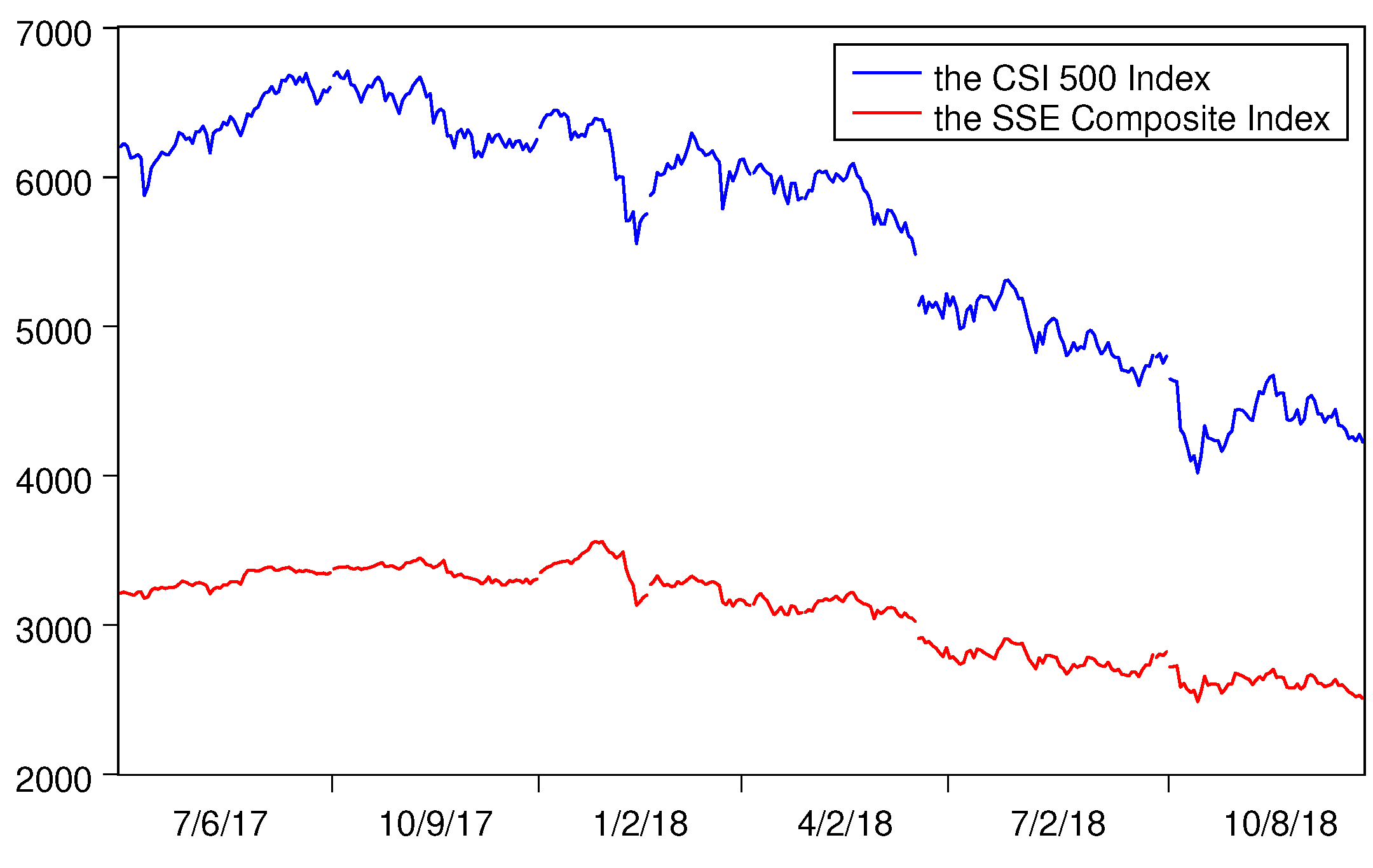
To verify the applicability of the proposed method to individual stocks with multiple price limits during the observation period, this paper focused on the period with high volatility in the market before COVID-19, from 6 July 2017, to 25 December 2018, a total of 362 trading days. From Figure 1, it can be seen that during the sample period, the CSI 500 Index showed a significant downward trend compared with the SSE Composite Index, with greater volatility (the breakpoint in the figure indicates that the day is not a trading day). Therefore, this paper targeted the constituent stocks of the CSI 500 Index and selected the price of ten stocks with a high number of limit up and limit down changes during the sample period as the research objects. Among them, stocks 600158.SH and 002273.SZ experienced multiple consecutive trading suspensions or equity distributions during the sample period. In order to avoid the possible impact of such events on the observation results, this paper removed them from the samples and observed the application effect of the change point detection method on the other eight stocks. The data employed in this paper were collected from the Wind database.

Table 1. Sample stocks and the number of their price limits.

Stock Code	600198	002405	002642	600651	600171	000762	300253	600536
Counts	11	11	12	7	7	10	12	18
	(5,6)	(7,4)	(5,7)	(1,6)	(4,3)	(6,4)	(9,3)	(12,6)

The first number in parentheses represents the number of times when the sample stock experienced a limit up change, while the second number represents the number of times when the sample stock experienced a limit down. The numbers outside the parentheses represent the total number of price limits.

shows the statistical data of the number of price limits that occurred in the closing of the sample stocks. During the research period, these eight sample stocks experienced 7 to 18 closing price limits. Existing studies have shown that the impact of the price limit on stock prices may have a volatility spillover effect [37,38], which suggests that its impact on prices will not only stay on the day when the price limit occurs but may extend several trading days later. In order to more effectively correct the impact of price limits on the time series of stock prices, this study investigated the correction of stock closing prices after five trading days from the day when the price limit occurred.

This paper adopted the Kalman filtering method by calculating the state vector $X_{t+1}$ in Equation (19) to obtain the predicted stock price (where the first element in vector $X_{t+1}$ is the predicted stock price), and the predicted price was replaced by the original price as a corrected price to correct the stock price time series under the influence of the price limit.

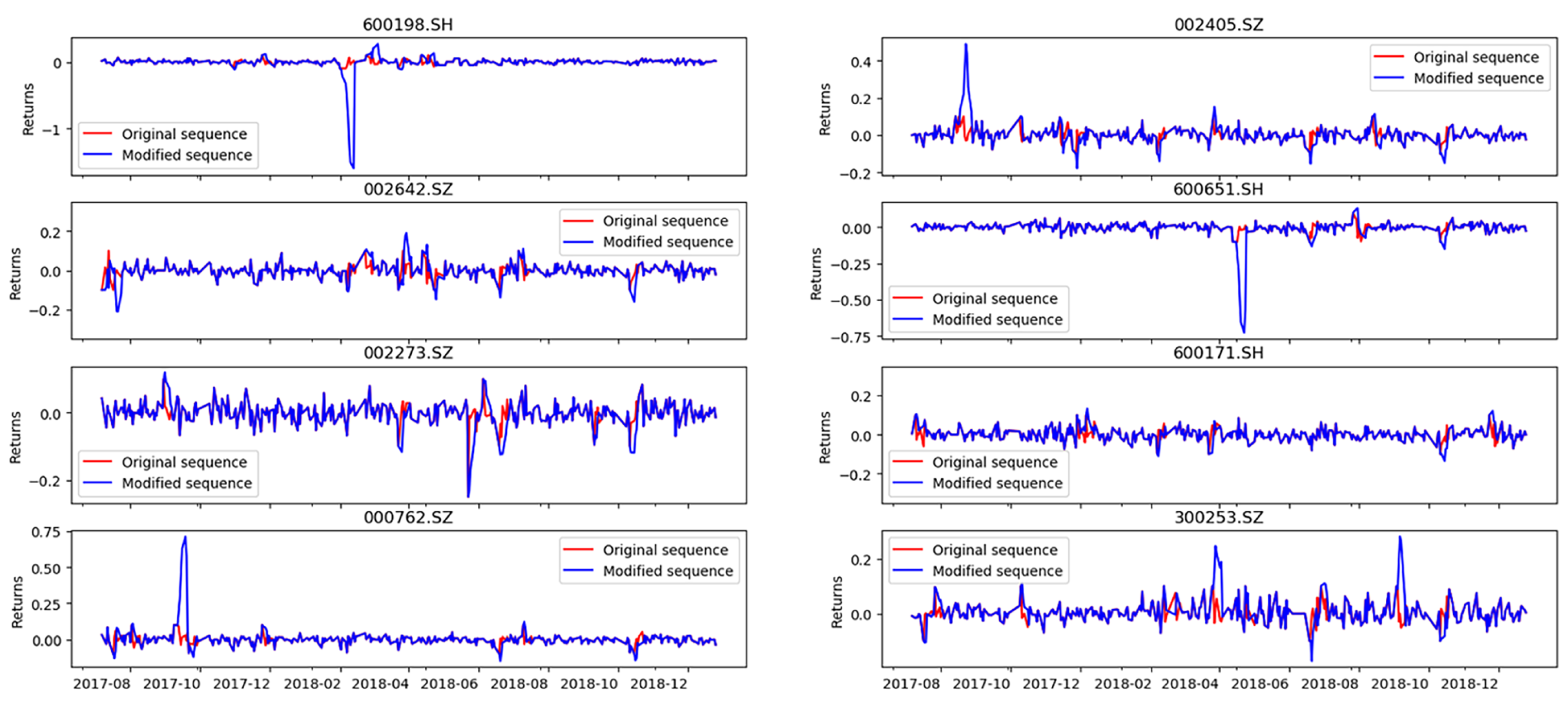
The corrected results are shown in Figure 2. For a more intuitive observation, Figure 2 reports the time-series comparison of stock price returns before and after correction. When $Returns=\pm 0.1$, t indicates that the stock has a price limit, the red line represents the return series of the original stock price, and the blue line represents the corrected return series of the stock price. From the comparison results, it is found that the impact of price limits on the market was not simply the suppression of volatility but also a magnetic attraction effect. This is because some stocks after the correction of the daily limit up or limit down changes were significantly higher than before the correction, and some stock prices after the correction of the daily price limit did not touch the daily price limit. At the same time, it is found that when the volatility reversal of the trading day after the price limit occurred, the reversal effect of the corrected stock price return was more severe than that of the pre-corrected stock price. This indirectly supports the view that the suppression effect of the price limit on volatility does exist, and the reduction in volatility that occurs after the limit up or limit down changes are not entirely determined by the reversal effect. The results in this paper only roughly imply this conclusion, and further research is needed to confirm this issue.

4.2. Change Point Detection

In order to test the effectiveness of the change point test method proposed in this paper, the study first conducted a single-change point test for sample stocks. By using the Bayes estimation method proposed above, the Bayes factor $B_{10}$ was estimated according to Equation (12), the existence of the change point was judged according to the judgment rule of the Bayes factor $B_{10}$ proposed by Jeffreys [33], and the change point position K was determined according to Equations (14) and (15). In the detection step, four unknown parameters, ${\mathcal{F}}_0$, $\gamma$, m, and $\beta$, were involved. ${\mathcal{F}}_0$ was determined by historical data, while the selection of $\gamma$, m, and $\beta$ was determined according to the dynamic characteristics of the time series. This paper mainly presents the results of the $\beta$-ARCH model, so in subsequent empirical research, $m\equiv 2$ can be obtained. The following first shows the detection results of the classic ARCH model when $\beta =1$. And the residuals $\gamma$ in the two cases follow a normal distribution ($\gamma =2$) and a Laplace distribution ($\gamma =1$). The test results are detailed in

Table 2. The residuals follow the change point test results of the Laplace distribution.

Stock Code		600198	002405	002642	600651	600171	000762	300253	600536
Original sequence	$B_{10}$	21.28	21.044	21.21	19.68	28.42	21.79	20.31	21.47
	K	178.69	180.58	179.68	180.78	167.04	180.31	179.86	180.36
	$Std$.	78.98	79.7	79.41	80.39	78.44	79.05	79.83	78.41
Modified sequence	$B_{10}$	24.72	26.76	25.39	23.75	28.95	25.63	25.2	26.86
	K	178.28	178.59	177.55	178.19	173.28	177.33	180.59	180.56
	$Std.$	80.15	78.19	80.75	78.15	70.11	85.3	75.11	79.55

and

Table 3. The residuals follow the normal distribution of change point detection results.

Stock Code		600198	002405	002642	600651	600171	000762	300253	600536
Original Sequence	$B_{10}$	195.17	1287.16	189.75	221.14	519.14	301.45	427.35	1350.88
	K	157.24	152.08	170.51	169.09	155.33	141.34	223.96	278.10
	$Std$.	72.51	72.97	69.54	80.26	55.74	69.22	75.97	72.26
Modified Sequence	$B_{10}$	227.63	611.61	357.78	237.38	5002.07	735.17	1412.78	198.70
	K	155.40	144.12	208.25	191.18	136.63	89.19	226.93	175.67
	$Std.$	78.87	63.97	72.56	69.56	28.39	80.93	50.23	76.79

.

From the test results in Table 2, which assume that the residual follows the Laplace distribution, the change points of both the original data and the revised data basically occur around $K=180$. The events that occurred near during this period that had a significant impact on the Chinese stock market included the following: (1) On 22 March, the Federal Reserve announced a rate hike (corresponding to the Chinese stock market on 23 March, $K=175$), and the international stock market plunged, with the SSE Composite Index decreasing by 3.39% and the SZI Composite Index decreasing by 4.02%. (2) On the evening of 29 March, the CSRC issued a CNY 100 million fine to two large retail investors (corresponding to the Chinese stock market on 30 March, $K=181$). This result shows that the location of the change point was basically in the middle of the two events, which is just in line with the information transmission effect of the stock market. The first event was triggered by economic policies in the United States, and there was a certain time delay in its transmission to the Chinese stock market, resulting in the measured change point position lagging behind the event time; the second event was triggered by the regulatory behavior of the CSRC, and there was relevant information transmission in the market before the event occurred, so that the change point position was earlier than the event. This result indicates that the change point detection method proposed in this paper has a good practical effect. From the comparison of the detection results before and after correction, it can be seen that six of eight stocks had a change point position closer to the time of the event (1) and earlier than the event (2). This shows that the position of the change points detected for the corrected data was better than the data before the correction. For the other two stocks, 300253.SZ and 600536.SH, the change point position difference before and after correction was less than 1, but the Bayes factor $B_{10}$ of the stock price after correction was increased, indicating that the revised data were more inclined to support the conclusion of the change point. The above results indicate that the position of a change point is better when the stock price is modified by the Kalman filter under the influence of the trading system.

In order to observe the effect of change point detection under the assumption that the residuals follow a normal distribution, a second test was conducted by setting m = 2, $\beta$ = 1, and $\gamma$ = 2 (see Table 3). The results show that compared with the Laplace distribution, the variability of the change point positions of the eight stocks increased, and they all deviated significantly from the time of event occurrence. This indicates that asset prices do have fat-tail characteristics, and the application of the generalized error distribution assumption is reasonable.

In order to further observe the performance of the $\beta$-ARCH model, this study has compiled the change point detection results under different values of $\beta$, as shown in

Table 4. The residuals follow the change point test results of the Laplace distribution when $\beta ={\displaystyle \frac{1}{4}}$.

Stock Code		600198	002405	002642	600651	600171	000762	300253	600536
Original sequence	$B_{10}$	119.02	225.81	145.63	87.63	146.29	150.88	128.76	226.85
	K	166.27	174.60	164.35	163.03	175.52	167.28	189.47	185.57
	$Std$.	80.78	78.39	80.00	78.80	79.06	78.98	80.09	80.84
Modified sequence	$B_{10}$	130.39	258.87	166.92	94.93	157.02	173.58	144.67	279.20
	K	164.85	170.06	158.86	164.27	175.52	162.16	188.18	187.26
	$Std.$	78.98	78.32	80.82	77.45	79.52	78.86	79.90	78.13

,

Table 5. The residuals follow the change point test results of the Laplace distribution when $\beta ={\displaystyle \frac{1}{2}}$.

Stock Code		600198	002405	002642	600651	600171	000762	300253	600536
Original sequence	$B_{10}$	68.77	106.11	78.66	555.64	79.14	80.69	72.58	106.51
	K	170.63	176.33	169.38	168.39	176.93	171.28	186.44	183.79
	$Std$.	80.77	79.09	80.26	79.48	79.55	79.55	80.23	80.72
Modified sequence	$B_{10}$	72.73	115.75	85.71	58.41	83.13	88.33	78.48	120.27
	K	169.89	173.54	166.01	169.20	176.89	167.85	185.39	184.43
	$Std.$	79.69	79.01	80.89	78.68	79.85	79.61	80.16	79.24

and

Table 6. The residuals follow the change point test results of the Laplace distribution when $\beta ={\displaystyle \frac{3}{4}}$.

Stock Code		600198	002405	002642	600651	600171	000762	300253	600536
Original sequence	$B_{10}$	68.77	106.11	78.66	555.64	79.14	80.69	72.58	106.51
	K	170.63	176.33	169.38	168.39	176.93	171.28	186.44	183.79
	$Std$.	80.77	79.09	80.26	79.48	79.55	79.55	80.23	80.72
Modified sequence	$B_{10}$	72.73	115.75	85.71	58.41	83.13	88.33	78.48	120.27
	K	169.89	173.54	166.01	169.20	176.89	167.85	185.39	184.43
	$Std.$	79.69	79.01	80.89	78.68	79.85	79.61	80.16	79.24

. As the value of $\beta$ gradually decreases, the time dispersion between the detected change point position and the occurrence of the financial core event increases, and the distance between the change point position before and after correction also increases accordingly. This implies that the classical ARCH model under the Laplace distribution assumption is more suitable for the test samples selected in this study.

4.3. Parameter Estimation of $\beta$-ARCH Model after Change Point Detection

To further confirm the effectiveness of change point detection, based on the previous research conclusions, parameter estimation was conducted on the segmented time series formed after single-change point detection under the conditions of $m=2$, $\beta =1$, and $\gamma =2$. The specific results are detailed in

Table 7. Comparison of parameter estimation of ARCH model before and after correction.

Stock Code	Original Sequence				Modified Sequence
	${\mathbf{\alpha }}_{\mathbf{0}}^{\prime }$	${\mathbf{\alpha }}_{\mathbf{1}}^{\prime }$	${\mathbf{\alpha }}_{\mathbf{0}}^{\ast }$	${\mathbf{\alpha }}_{\mathbf{1}}^{\ast }$	${\mathbf{\alpha }}_{\mathbf{0}}^{\prime }$	${\mathbf{\alpha }}_{\mathbf{1}}^{\prime }$	${\mathbf{\alpha }}_{\mathbf{0}}^{\ast }$	${\mathbf{\alpha }}_{\mathbf{1}}^{\ast }$
600198	$9.1\times {10}^{-4}$	0.39	$7.8\times {10}^{-4}$	0.09	$6.9\times {10}^{-4}$	1.00	$7.2\times {10}^{-4}$	0.13
	(3.63)	(2.22)	(6.62)	(1.26)	(3.49)	(3.52)	(6.84)	(1.48)
002405	$6.1\times {10}^{-4}$	0.20	$7.8\times {10}^{-4}$	0.02	$1.4\times {10}^{-3}$	1.00	$6.4\times {10}^{-4}$	0.48
	(6.23)	(1.19)	(5.64)	(0.28)	(2.23)	(2.00)	(5.34)	(2.54)
002642	$2.2\times {10}^{-3}$	0.37	$6.9\times {10}^{-4}$	0.27	$1.7\times {10}^{-3}$	1.00	$5.8\times {10}^{-4}$	0.58
	(1.04)	(0.78)	(4.90)	(2.27)	(1.31)	(1.32)	(4.88)	(3.24)
600651	$5.2\times {10}^{-4}$	0.08	$7.0\times {10}^{-4}$	0.20	$5.2\times {10}^{-4}$	0.073	$1.7\times {10}^{-3}$	0.80
	(6.38)	(0.97)	(5.08)	(2.00)	(6.46)	(0.93)	(2.84)	(2.41)
600171	$1.0\times {10}^{-3}$	0.02	$8.6\times {10}^{-4}$	0.06	$9.4\times {10}^{-4}$	0.14	$5.2\times {10}^{-4}$	0.20
	(5.63)	(0.16)	(5.71)	(0.84)	(5.91)	(1.99)	(7.79)	(2.41)
000762	$1.0\times {10}^{-3}$	0.22	$5.2\times {10}^{-4}$	0.07	$7.3\times {10}^{-4}$	0.61	$3.9\times {10}^{-3}$	0.39
	(3.71)	(1.10)	(5.30)	(0.94)	(3.39)	(2.06)	(16.79)	(0.95)
300253	$1.4\times {10}^{-3}$	0.25	$1.4\times {10}^{-3}$	0.05	$9.1\times {10}^{-4}$	0.79	$1.9\times {10}^{-3}$	0.62
	(1.14)	(0.70)	(4.37)	(0.41)	(1.78)	(1.36)	(1.83)	(1.43)
600536	$6.4\times {10}^{-4}$	0.29	$1.7\times {10}^{-3}$	0.22	$5.4\times {10}^{-4}$	0.59	$9.8\times {10}^{-4}$	1.00
	(2.75)	(1.14)	(4.00)	(1.36)	(3.43)	(2.15)	(5.09)	(5.07)

, where ${\alpha }_0^{\prime }$ and ${\alpha }_0^{\ast }$ are the ARCH model constant term parameters of the two time series before and after the change point, ${\alpha }_0^{\prime }$ and ${\alpha }_0^{\ast }$ are the ARCH model lag first-order term parameters of the two time series before and after the change point, and the numbers in brackets are the t values of the parameter statistics. From the estimation results of the original data, it can be seen that the constant terms of the estimation model before and after the change point were mostly significant but the values were small. The parameter ${\alpha }_1$ of the lag first-order term of the ARCH model had a significant difference in only three stocks, 600198.SH, 002642.SZ, and 600651.SH. However, in the data corrected by Kalman filtering, seven out of eight stocks showed significant changes in the ARCH model parameters before and after the change point. This indicates that it is easier to detect the change point in the market after the Kalman filter is used to correct the stock price of the stock that has limit up and limit down changes during the observation period.

5. Conclusions

This paper proposes an effective change point detection method for China’s stock market, which is in a period of significant volatility. The study first used the Bayes method to derive a change point detection method for the ARCH models, which is based on the Bayes factor $B_{10}$ to judge whether the change point exists, and the estimation method for the expected value and the standard deviation of the change point position parameter K were given. According to the Bayes factor based change point identification rule determined by Jeffreys, we notice that $B_{10}$ is not suitable for general change point detection problems and is only applicable to stocks with large fluctuations in limit up and limit down changes. On this basis, in view of the short-term distortion of stock price output caused by the trading system of price limits, the Kalman filter method is proposed to correct the influence of short-term distortion of stock prices on the detection of change point position.

The study employed the observation period from 6 July 2017 to 25 December 2018 (when the market was in a period of significant volatility), as the research observation period and selected the price of eight stocks with a high number of limit up and limit down changes in the constituent stocks of the CSI 500 Index to test the effectiveness of the method proposed in the paper. The conclusions are as follows: (1) The change point detection method proposed in this paper can determine that there exists a large-scale economic event in the market that may change the market trend near the change point location. The change point detection of the $\beta$-ARCH model based on the Bayes method proposed in this paper is reliable. (2) During periods of significant market volatility, the volatility of stock prices has leptokurtic characteristics. Using the assumption of a generalized error distribution to estimate the parameters of change point detection makes the results more reliable. (3) The short-term distortion caused by the price limit can lead to errors in the long-term observations of stock prices. After using the Kalman filtering method to correct short-term stock price distortions, the effectiveness of the proposed change point detection method is further improved. (4) The indirect results of the study suggest that the price limit trading system has both a magnetic effect and a fluctuation inhibitory effect on the market. This conclusion needs to be further confirmed in follow-up studies.

References

1. Liu, X.X.; Fang, L.; Zhang, Y.; Tang, P. Liquidity Change-points Detection of Sovereign Debt Crisis in Europe and the United States Based on the Analysis of Stock Market. J. Manag. Sci. China 2014, 7, 82–94. [Google Scholar]
2. Greenwald, B.C.; Stein, J.C. Transaction Risk, Market Crashes and the Role of Circuit Breakers. J. Bus. 1991, 64, 443–462. [Google Scholar] [CrossRef]
3. Subrahmanyam, A. Circuit Breakers and Market Volatility: A Theoretical Perspective. J. Financ. 1994, 49, 237–254. [Google Scholar] [CrossRef]
4. Ryoo, H.J.; Smith, G. Korean Stock Prices under Price Limits: Variance Ratio Tests of Random Walks. Appl. Financ. Econ. 2002, 12, 545–553. [Google Scholar] [CrossRef]
5. Fisher, L. Some New Stock-Market Indexes. J. Bus. 1966, 1, 191–225. [Google Scholar] [CrossRef]
6. Harris, L.A. The October 1987 S & P 500 Stock-Futures Basis. J. Financ. 1989, 44, 77–99. [Google Scholar]
7. Page, E.S. Continuous Inspection Schemes. Biometrika 1954, 41, 100–115. [Google Scholar] [CrossRef]
8. Kokoszka, P.; Leipus, R. Testing for Parameter Changes in ARCH Models. Lith. Math. J. 1999, 39, 182–195. [Google Scholar] [CrossRef]
9. Kokoszka, P.; Leipus, R. Change-Point Estimation in ARCH Models. Bernoulli 2000, 6, 513–539. [Google Scholar] [CrossRef]
10. Lee, S.; Ha, J.; Na, O.Y.; Na, S.R. The Cusum Test for Parameter Change in Time Series Models. Scand. J. Stat. 2003, 30, 781–796. [Google Scholar] [CrossRef]
11. Lee, S.; Tokutsu, Y.; Maekawa, K. The Cusum Test for Parameter Change in Regression Models with ARCH Errors. J. Jpn. Stat. Soc. 2004, 34, 173–188. [Google Scholar] [CrossRef]
12. Lee, S.; Park, S. The Monitoring Test for the Stability of Regression Models with Nonstationary Regressors. Econ. Lett. 2009, 105, 250–252. [Google Scholar] [CrossRef]
13. Kim, S.; Cho, S.; Lee, S. On the Cusum Test for Parameter Changes in GARCH (1, 1) Models. Commun. Stat. Theory Methods 2000, 29, 445–462. [Google Scholar] [CrossRef]
14. Andreou, E.; Ghysels, E. Monitoring Disruptions in Financial Markets. J. Econom. 2006, 135, 77–124. [Google Scholar] [CrossRef]
15. Carsoule, F.; Franses, P.H. Monitoring Structural Change in Variance, with an Application to European Nominal Exchange Rate Volatility. Econom. Inst. Rep. 1999, 6, 1–33. [Google Scholar]
16. Berkes, I.; Gombay, E.; Horvath, L.; Kokoszka, P. Sequential Change-Point Detection in GARCH (p, q) Models. Econom. Theory 2004, 20, 1140–1167. [Google Scholar] [CrossRef]
17. Bardet, J.M.; Kengne, W. Monitoring Procedure for Parameter Change in Causal Time Series. J. Multivar. Anal. 2014, 125, 204–221. [Google Scholar] [CrossRef]
18. Horvath, L.; Kokoszka, P.; Teyssiere, G. Empirical Process of the Squared Residuals of an ARCH Sequence. Ann. Stat. 2001, 29, 445–469. [Google Scholar] [CrossRef]
19. Na, O.; Lee, Y.; Lee, S. Monitoring Parameter Change in Time Series Models. Stat. Methods Appl. 2011, 20, 171–199. [Google Scholar] [CrossRef]
20. Lai, T.L.; Xing, H. Stochastic Change-Point ARX-GARCH Models and Their Applications to Econometric Time Series. Stat. Sin. 2013, 23, 1573–1594. [Google Scholar] [CrossRef]
21. Wang, X.; Wang, Y.; Wang, D.; Liu, X. Modeling Short-term Post-offering Price-volume Relationships using Bayesian Change-point Panel Quantile Regression. Appl. Stoch. Models Bus. Ind. 2016, 32, 259–272. [Google Scholar] [CrossRef]
22. Fryzlewicz, P.; Subba Rao, S. Multiple-Change-Point Detection for Autoregressive Conditional Heteroscedastic Processes. J. R. Stat. Soc. Ser. B Stat. Methodol. 2014, 76, 925–947. [Google Scholar] [CrossRef]
23. Cho, H.; Fryzlewicz, P. Multiple-Change-Point Detection for High Dimensional Time Series via Sparsified Binary Segmentation. J. R. Stat. Soc. Ser. B Stat. Methodol. 2015, 77, 475–507. [Google Scholar] [CrossRef]
24. Chen, S.; Li, Y.X.; Kim, J.; Kim, S.W. Bayesian Change Point Analysis for Extreme Daily Precipitation. Int. J. Climatol. 2017, 37, 3123–3137. [Google Scholar] [CrossRef]
25. Monfared, M.E.D.; Lak, F. Bayesian Estimation of the Change Point in a Gamma Process using (X) Over-bar Control Chart. Commun. Stat. Simul. Comput. 2017, 46, 2333–2345. [Google Scholar] [CrossRef]
26. Bianchi, D.; Massimo, G.; Francesco, R. Macroeconomic Factors Strike Back: A Bayesian Change-Point Model of Time-Varying Risk Exposures and Premia in the US Cross-Section. J. Bus. Econ. Stat. 2017, 35, 110–129. [Google Scholar] [CrossRef]
27. Jung, M.; Song, S.; Chung, Y. Bayesian Change-point Problem using Bayes Factor with Hierarchical Prior Distribution. Commun. Stat. Theory Methods 2017, 46, 1352–1366. [Google Scholar] [CrossRef]
28. Chai, J.; Lu, Q.Y.; Hu, Y.; Wang, S.; Lai, K.K.; Liu, H. Analysis and Bayes Statistical Probability Inference of Crude Oil Price Change Point. Technol. Forecast. Soc. Chang. 2018, 126, 271–283. [Google Scholar] [CrossRef]
29. Guégan, D.; Diebolt, J. Probabilistic Properties of the β-ARCH Model. Stat. Sin. 1994, 4, 71–87. [Google Scholar]
30. Engle, R.F. Autoregressive conditional heteroscedasticy with estimates of the variance of U.K. inflation. Econometrica 1982, 50, 987–1008. [Google Scholar] [CrossRef]
31. Nadarajah, S. A Generalized Normal Distribution. J. Appl. Stat. 2005, 32, 685–694. [Google Scholar] [CrossRef]
32. Kass, R.E.; Raftery, A.E. Bayes Factors. J. Am. Stat. Assoc. 1995, 90, 773–795. [Google Scholar] [CrossRef]
33. Jeffreys, H. Theory of Probability, 3rd ed.; Clarendon Press: Oxford, UK, 1961. [Google Scholar]
34. Harvey, A.C. Time Series Models, 2nd ed.; MIT Press: Cambridge, MA, USA, 1995; Volume 158, p. 191. [Google Scholar]
35. Rankin, J.M. Kalman Filtering Approach to Market Price Forecasting; Iowa State University: Ames, IA, USA, 1986; pp. 40–52. [Google Scholar]
36. Durbin, J.; Koopman, S.J. Time Series Analysis by State Space Methods: Second Edition. Siem Jan Koopman 2012, 39, 255–256. [Google Scholar]
37. Wu, L.X.; Xu, L.B. Does the Price Limit is a Behavior which Distorted the Stock Value?— New Evidence from the China Stock Market. China Account. Financ. Rev. 2002, 2, 1–21. [Google Scholar]
38. Liu, J.J.; Du, J.; Chen, J.W. The Effect of the Price Limit in China’s Stock Market. Stat. Decis. 2006, 16, 114–116. [Google Scholar]
Figure 1. Time series of the CSI 500 Index and the SSE Composite Index.
Axioms 13 00643 g001
Figure 2. Comparison of sample stock returns before and after Kalman filtering correction.
Axioms 13 00643 g002