Article

Ensuring Topological Data-Structure Preservation under Autoencoder Compression Due to Latent Space Regularization in Gauss–Legendre Nodes

by
Chethan Krishnamurthy Ramanaik
1,*,†,
Anna Willmann
2,†,
Juan-Esteban Suarez Cardona
2,
Pia Hanfeld
2,
Nico Hoffmann
3 and
Michael Hecht
2,4,*
1
Forschungsinstitut CODE, University of the Bundeswehr Munich, 85579 Neubiberg, Germany
2
CASUS—Center for Advanced Systems Understanding, Helmholtz-Zentrum Dresden-Rossendorf e.V. (HZDR), 01328 Dresden, Germany
3
SAXONY.ai, 01217 Dresden, Germany
4
Mathematical Institute, University of Wrocław, 50-384 Wrocław, Poland
*
Authors to whom correspondence should be addressed.
These authors contributed equally to this work.
Axioms 2024, 13(8), 535; https://doi.org/10.3390/axioms13080535
Submission received: 3 June 2024 / Revised: 5 July 2024 / Accepted: 27 July 2024 / Published: 7 August 2024
(This article belongs to the Special Issue Differential Geometry and Its Application, 2nd Edition)

Abstract

:
We formulate a data-independent latent space regularization constraint for general unsupervised autoencoders. The regularization relies on sampling the autoencoder Jacobian at Legendre nodes, which are the centers of the Gauss–Legendre quadrature. Revisiting this classic allows us to prove that regularized autoencoders ensure a one-to-one re-embedding of the initial data manifold into its latent representation. Demonstrations show that previously proposed regularization strategies, such as contractive autoencoding, cause topological defects even in simple examples, as do convolutional-based (variational) autoencoders. In contrast, topological preservation is ensured by standard multilayer perceptron neural networks when regularized using our approach. This observation extends from the classic FashionMNIST dataset to (low-resolution) MRI brain scans, suggesting that reliable low-dimensional representations of complex high-dimensional datasets can be achieved using this regularization technique.
MSC:
53A07; 57R40; 53C22

1. Introduction

Systematic analysis and post-processing of high-dimensional and high-throughput datasets [1,2] is a current computational challenge across disciplines such as neuroscience [3,4,5], plasma physics [6,7,8], and cell biology and medicine [9,10,11,12]. In the machine learning (ML) community, autoencoders (AEs) are commonly considered the central tool for learning a low-dimensional one-to-one representation of high-dimensional datasets. These representations serve as a baseline for feature selection and classification tasks, which are prevalent in bio-medicine [13,14,15,16,17].
AEs can be considered as a non-linear extension of classic principal component analysis (PCA) [18,19,20]. Comparisons for linear problems are provided in [21]. While addressing the non-linear case, AEs face the challenge of preserving the topological data structure under AE compression.
To state the problem: We mathematically formalize AEs as pairs of continuously differentiable maps ( φ , ν ) , φ : Ω m 2 Ω m 1 , ν : Ω m 1 Ω m 2 , 0 < m 1 < m 2 N , defined on bounded domains Ω m 1 R m 1 and Ω m 2 R m 2 . Commonly, φ is termed the encoder, and ν the decoder. We assume that the data D D is sampled from a regular or even smooth data manifold D Ω m 2 , with dim D = m 0 m 1 .
We seek to find proper AEs ( φ , ν ) yielding homeomorphic latent representations φ ( D ) = D D . In other words, the restrictions φ | D : D D and ν | D : D D of the encoder and decoder result in one-to-one maps, being inverse to each other:
D D = φ ( D ) Ω m 1 , ν ( φ ( x ) ) = x , for all x D .
While the second condition in Equation (1) is usually realized by minimization of a reconstruction loss, this is insufficient for guaranteeing the one-to-one representation D D .
To realize AEs matching both requirements in Equation (1), we strengthen the condition by requiring the decoder to be an embedding of the whole latent domain Ω m 1 D , including ν ( Ω m 1 ) D in its interior. See Figure 1 for an illustration. We mathematically prove and empirically demonstrate this latent regularization strategy to deliver regularized AEs (AR-REG), satisfying Equation (1).
Our investigations are motivated by recent results of Hansen et al. [22,23,24], complementing other contributions [25,26,27] that investigate instabilities of machine learning methods from a general mathematical perspective.

1.1. The Inherent Instability of Inverse Problems

The instability phenomenon of inverse problems states that, in general, one cannot guarantee solutions of inverse problems to be stable. An excellent introduction to the topic is given in [22] with deeper treatments and discussions in [23,24].
In our setup, these insights translate to the fact that, in general, the local Lipschitz constant
L ε ( ν , y ) = sup 0 < y y < ε ν ( y ) ν ( y ) y y , ε > 0
of the decoder ν : Ω m 1 Ω m 2 at some latent code y Ω 1 might be unbounded. Consequently, small perturbations y y of the latent code can result in large differences of the reconstruction ν ( y ) ν ( y ) 0 . This fact generally applies and can only be avoided if an additional control on the null space of the Jacobian of the encoder ker J ( φ ( x ) ) is given. Providing this control is the essence of our contribution.

1.2. Contribution

Avoiding the aforementioned instability, requires the null space of the Jacobian of the encoder ker J ( φ ) to be perpendicular to the tangent space of D
ker J ( φ ) T D .
In fact, due to the inverse function theorem, see, e.g., [28,29], the conditions Equations (1) and (2) are equivalent. In Figure 1, ker J ( φ ) is illustrated to be perpendicular to the image of the whole latent domain Ω m 1
ker J ( φ ) T ν ( Ω m 1 ) , ν ( Ω m 1 ) D ,
being sufficient for guaranteeing Equation (2), and consequently, Equation (1).
While several state-of-the-art AE regularization techniques are commonly established, none of them specifically formulates this necessary mathematical requirement in Equation (2). Consequently, we are not aware of any regularization approach that can theoretically guarantee the regularized AE to preserve the topological data-structure, as we do in Theorem 1. Our computational contributions split into:
(C1) 
For realising a latent space regularized AE (AE-REG) we introduce the L 2 -regularization loss
L reg ( φ , ν ) = J ( φ ν ) I L 2 ( Ω m 1 ) 2
and mathematically prove the AE-REG to satisfy condition Equation (1), Theorem 1, when being trained due to this additional regularization.
(C2) 
To approximate L reg ( φ , ν ) we revisit the classic Gauss–Legendre quadratures (cubatures) [30,31,32,33,34], only requiring sub-sampling of J ( ν φ ) ( p α ) , p α P m , n on a Legendre grid of sufficient high resolution 1 | P m , n | in order to execute the regularization. While the data-independent latent Legendre nodes P m , n Ω m 1 are contained in the smaller dimensional latent space, regularization of high resolution can be efficiently realised.
(C3) 
Based on our prior work [35,36,37], and [38,39,40,41], we complement the regularization through a hybridisation approach combining autoencoders with multivariate Chebyshev-polynomial-regression. The resulting Hybrid AE is acting on the polynomial coefficient space, given by pre-encoding the training data due to high-quality regression.
We want to emphasize that the proposed regularization is data-independent in the sense that it does not require any prior knowledge of the data manifold, its embedding, or any parametrization of D . Moreover, while being integrated into the loss function, the regularization is independent of the AE architecture and can be applied to any AE realizations, such as convolutional or variational AEs. Our results show that already regularized MLP-based AEs perform superior to these alternatives.
As we demonstrate, the regularization yields the desired re-embedding, enhances the autoencoder’s reconstruction quality, and increases robustness under noise perturbations.

1.3. Related Work—Regularization of Autoencoders

A multitude of supervised learning schemes, addressing representation learning tasks, are surveyed in [42,43]. Self-supervised autoencoders rest on inductive bias learning techniques [44,45] in combination with vectorized autoencoders [46,47]. However, the mathematical requirements, Equations (1) and (2) were not considered in these strategies at all. Consequently, one-to-one representations might only be realized due to a well-chosen inductive bias regularization for rich datasets [9].
This article focus on regularization techniques of purely unsupervised AEs. We want to mention the following prominent approaches:
(R1) 
Contractive AEs (ContraAE) [48,49] are based on an ambient Jacobian regularization loss
L reg ( φ , ν ) = J ( ν φ ) I L 2 ( Ω m 2 ) 2
formulated in the ambient domain. This makes contraAEs arbitrarily contractive in perpendicular directions ( T D ) of T D . However, this is insufficient to guarantee Equation (1). In addition, the regularization is data dependent, resting on the training dataset, and is computationally costly due to the large Jacobian J R m 2 × m 2 , m 2 m 1 1 . Several experiments in Section 5 demonstrate contraAE failing to deliver topologically preserved representations.
(R2) 
Variational AEs (VAE), along with extensions like β -VAE, consist of stochastic encoders and decoders and are commonly used for density estimation and generative modelling of complex distributions based on minimisation of the Evidence Lower Bound (ELBO) [50,51]. The variational latent space distribution induces an implicit regularization, which is complemented by [52,53] due to a l 1 -sparsity constraint of the decoder Jacobian.
However, as the contraAE-constraint, this regularization is computationally costly and insufficient for guaranteeing a one-to-one encoding, which is reflected in the degenerated representations appearing in Section 5.
(R3) 
Convolutional AEs (CNN-AE) are known to deliver one-to-one representations for a generic setup theoretically [54]. However, the implicit convolutions seems to prevent clear separation of tangent T D and perpendicular direction ( T D ) of the data manifold D , resulting in topological defects already for simple examples, see Section 5.

2. Mathematical Concepts

We provide the mathematical notions on which our approach rests, starting by fixing the notation.

2.1. Notation

We consider neural networks (NNs) ν ( · , w ) of fixed architecture Ξ m 1 , m 2 , specifying number and depth of the hidden layers, the choice of piece-wise smooth activation functions σ ( x ) , e.g., ReLU or sin, with input dimension m 1 and output dimension m 2 . Further, Υ Ξ m 1 , m 2 denotes the parameter space of the weights and bias w = ( v , b ) W = V × B R K , K N , see, e.g., [55,56].
We denote with Ω m = ( 1 , 1 ) m the m-dimensional open standard hypercube, with · the standard Euclidean norm on R m and with · p , 1 p the l p -norm. Π m , n = span { x α } α n denotes the R -vector space of all real polynomials in m variables spanned by all monomials x α = i = 1 m x i α i of maximum degree  n N and A m , n = { α N m : α = max i = 1 , , m { | α i | } n } the corresponding multi-index set. For an excellent overview on functional analysis we recommend [57,58,59]. Here, we consider the Hilbert space L 2 ( Ω m , R ) of all Lebesgue measurable functions f : Ω m R with finite L 2 -norm f L 2 ( Ω m ) 2 < induced by the inner product
< f , g > L 2 ( Ω m ) = Ω m f · g d Ω m , f , g L 2 ( Ω , R ) .
Moreover, C k ( Ω m , R ) , k N { } denotes the Banach spaces of continuous functions being k-times continuously differentiable, equipped with the norm
f C k ( Ω m ) = i = 0 k sup x Ω m | D α f ( x ) | , α 1 k .

2.2. Orthogonal Polynomials and Gauss–Legendre Cubatures

We follow [30,31,32,33,60] for recapturing: Let m , n N and P m , n = i = 1 m Leg n Ω m be the m-dimensional Legendre grids, where Leg n = { p 0 , , p n } are the n + 1  Legendre nodes given by the roots of the Legendre polynomials of degree n + 2 . We denote p α = ( p α 1 , , p α m ) P A m , n , α A m , n . The Lagrange polynomials L α Π A m , n , defined by L α ( p β ) = δ α , β , α , β A m , n , where δ · , · denotes the Kronecker delta, are given by
L α = i = 1 m l α i , i , l j , i = j i , j = 0 m x i p j p i p j .
Indeed, the L α are an orthogonal L 2 -basis of Π m , n ,
L α , L β L 2 ( Ω m ) = Ω m L α ( x ) L β ( x ) d Ω m = w α δ α , β ,
where the Gauss–Legendre cubature weight  w α = L α L 2 ( Ω m ) 2 can be computed numerically. Consequently, for any polynomial Q Π m , 2 n + 1 of degree 2 n + 1 the following cubature rule applies:
Ω m Q ( x ) d Ω m = α A m , n w α Q ( p α ) .
Thanks to | P m , n | = ( n + 1 ) m ( 2 n + 1 ) m this makes Gauss–Legendre integration a very powerful scheme, yielding
Q 1 , Q 2 L 2 ( Ω m ) = α A m , n Q 1 ( p α ) Q 2 ( p α ) w α ,
for all Q 1 , Q 2 Π m , n .
In light of this fact, we propose the following AE regularization method.

3. Legendre-Latent-Space Regularization for Autoencoders

The regularization is formulated from the perspective of classic differential geometry, see, e.g., [28,61,62,63]. As introduced in Equation (1), we assume that the training data D train D R m 2 is sampled from a regular data manifold. We formalise the notion of autoencoders:
Definition 1
(autoencoders and data manifolds). Let 1 m 0 m 1 m 2 N , D Ω m 2 be a (data) manifold of dimension dim D = m 0 . Given continuously differentiable maps φ : Ω m 2 Ω m 1 , ν : Ω m 1 Ω m 2 such that:
(i) 
ν is a right-inverse of φ on D , i.e, ν ( φ ( x ) ) = x for all x D .
(ii) 
φ is a left-inverse of ν, i.e, φ ( ν ( y ) ) = y for all y Ω m 1
Then we call the pair ( φ , ν ) a proper autoencoder with respect to D .
Given a proper AE ( φ , ν ) , φ yields a low dimensional homeomorphic re-embedding of D D = φ ( D ) R m 1 as demanded in Equation (1) and illustrated in Figure 1, fulfilling the stability requirement of Equation (2).
We formulate the following losses for deriving proper AEs:
Definition 2
(regularization loss). Let D Ω m 2 be a C 1 -data manifold of dimension dim D = m 0 < m 1 < m 2 and D train D be a finite training dataset. For NNs φ ( · , u ) Ξ m 2 , m 1 , ν ( · , w ) Ξ m 1 , m 2 with weights ( u , w ) Υ Ξ m 2 , m 1 × Υ Ξ m 1 , m 2 , we define the loss
L D train , n : Υ Ξ m 2 , m 1 × Υ Ξ m 1 , m 2 R + , L D train , n ( u , w ) = L 0 ( D train , u , w ) + λ L 1 ( u , w , n ) ,
where λ > 0 is a hyper-parameter and
L 0 ( D train , u , w ) = x D train x ν ( φ ( x , u ) , w ) 2
L 1 ( u , w , n ) = α A m 1 , n I J φ ( ν ( p α , w ) , u ) 2 ,
with I R m 1 × m 1 denoting the identity matrix, p α P m 1 , n be the Legendre nodes, and J φ ( ν ( p α , w ) R m 1 × m 1 the Jacobian.
We show that the AEs with vanishing loss result to be proper AEs, Defintion 1.
Theorem 1
(Main Theorem). Let the assumptions of Definition 2 be satisfied, and φ ( · , u n ) Ξ m 2 , m 1 , ν ( · , w n ) Ξ m 1 , m 2 be sequences of continuously differentiable NNs satisfying:
(i) 
The loss converges L D train , n ( u n , w n ) n 0 .
(ii) 
The weight sequences converge
lim n ( u n , w n ) = ( u , w ) Υ Ξ m 2 , m 1 × Υ Ξ m 1 , m 2 .
(iii) 
The decoder satisfies ν ( Ω m 1 , w n ) D , n n 0 N for some n 0 1 .
Then ( φ ( · , w n ) , ν ( · , u n ) ) n ( φ ( · , w ) , ν ( · , u ) ) uniformly converges to a proper autoencoder with respect to D .
Proof. 
The proof follows by combining several facts: First, the inverse function theorem [29] implies that any map ρ C 1 ( Ω m , Ω m ) satisfying
J ( ρ ( x ) ) = I , x Ω m , and ρ ( x 0 ) = x 0 ,
for some x 0 Ω m is given by the identity, i.e., ρ ( x ) = x , x Ω m .
Secondly, the Stone–Weierstrass theorem [64,65] states that any continuous map ρ C 0 ( Ω m , Ω m ) , with coordinate functions ρ ( x ) = ( ρ 1 ( x ) , , ρ m ( x ) ) can be uniformly approximated by a polynomial map Q ρ n ( x ) = ( Q ρ , 1 n ( x ) , , Q ρ , m n ( x ) ) , Q ρ , i n ( x ) Π m , n , 1 i m , i.e, ρ Q ρ n C 0 ( Ω m ) n 0 .
Thirdly, while the NNs φ ( · , w ) , ν ( · , u ) depend continuously on the weights u , w , the convergence in ( i i ) is uniform. Consequently, the convergence L D train , n ( u n , w n ) n 0 of the loss implies that any sequence of polynomial approximations Q ρ n ( x ) of the map ρ ( · ) = φ ( ν ( · , w ) , u ) satisfies
α A m 1 , n I J Q ρ n ( p α ) 2 = 0
in the limit for n . Hence, Equation (12) holds in the limit for n and consequently φ ( ν ( y , w ) , u ) = Q ρ ( y ) = y for all y Ω m 1 yielding requirement ( i i ) of Definition 1.
Given that assumption ( i i i ) is satisfied, in completion, requirement ( i ) of Definition 1 holds, finishing the proof. □
Apart from ensuring topological maintenance, one seeks for high-quality reconstructions. We propose a novel hybridization approach, delivering both.

4. Hybridization of Autoencoders Due to Polynomial Regression

The hybridisation approach rests on deriving Chebyshev Polynomial Surrogate Models  Q Θ , d fitting the initial training data d D train Ω m 2 . For the sake of simplicity, we motivate the setup in case of images:
Let d = ( d i j ) 1 i , j r R r × r be the intensity values of an image on an equidistant pixel grid G r × r = ( g i j ) 1 i , j r Ω 2 of resolution r × r , r N . We seek for a polynomial
Q Θ : Ω 2 R , Q Θ Π 2 , n ,
such that evaluating Q Θ , Θ = ( θ α ) α A 2 , n R | A 2 , n | on G r × r approximates d, i.e., Q Θ ( g i j ) d i j for all 1 i , j r . We model Q Θ in terms of Chebyshev polynomials of first kind well known to provide excellent approximation properties [33,35]:
Q Θ ( x 1 , x 2 ) = α A 2 , n θ α T α 1 ( x 1 ) T α 2 ( x 2 ) .
The expansion is computed due to standard least-square fits:
Θ d = argmin C R | A 2 , n | R C d 2 ,
where R = ( T α ( g i j ) ) 1 i , j , n , α A 2 , n R r 2 × | A 2 , n | , T α = T α 1 · T α 2 denotes the regression matrix.
Given that each image (training point) d D train can be approximated with the same polynomial degree n N , we posterior train an autoencoder φ , ν , only acting on the polynomial coefficient space φ : R | A 2 , n | Ω m 1 , ν Ω m 1 R | A 2 , n | by exchanging the loss in Equation (10) due to
L 0 ( D train , u , w ) = d D train d R · ν ( φ ( Θ d , u ) , w ) 2
In contrast to the regularization loss in Definition 2, here, pre-encoding the training data due to polynomial regression decreases the input dimension m 2 N of the (NN) encoder φ : Ω m 2 Ω m 1 . In practice, this enables to reach low dimensional latent dimension by increasing the reconstruction quality, as we demonstrate in the next section.

5. Numerical Experiments

We executed experiments, designed to validate our theoretical results, on hemera a NVIDIA V100 cluster at HZDR. Complete code benchmark sets and supplements are available at https://github.com/casus/autoencoder-regularisation, accessed on 2 June 2024. The following AEs were applied:
(B1) 
Multilayer perceptron autoencoder (MLP-AE): Feed forward NNs with activation functions σ ( x ) = sin ( x ) .
(B2) 
Convolutional autoencoder (CNN-AE): Standard convolutional neural networks (CNNs) with activation functions σ ( x ) = sin ( x ) , as discussed in (R3).
(B3) 
Variational autoencoder: MLP based (MLP-VAE) and CNN based (CNN-VAE) as in [50,51], discussed in (R2).
(B4) 
Contractive autoencoder (ContraAE): MLP based with with activation functions σ ( x ) = sin ( x ) as in [48,49], discussed in (R1).
(B5) 
regularized autoencoder (AE-REG): MLP based, as in (B1), trained with respect to the regularization loss from Definition 2.
(B6) 
Hybridised AE (Hybrid AE-REG): MLP based, as in (B1), trained with respect to the modified loss in Definition 2 due to Equation (15).
The choice of activation functions σ ( x ) = sin ( x ) yields a natural way for normalizing the latent encoding to Ω m and performed best compared to trials with ReLU, ELU or σ ( x ) = tanh ( x ) . The regularization of AE-REG and Hybrid AE-REG is realized due to sub-sampling batches from the Legendre grid P m , n for each iteration and computing the autoencoder Jacobians due to automatic differentiation [66].

5.1. Topological Data-Structure Preservation

Inspired by Figure 1, we start by validating Theorem 1 for known data manifold topologies.
Experiment 1
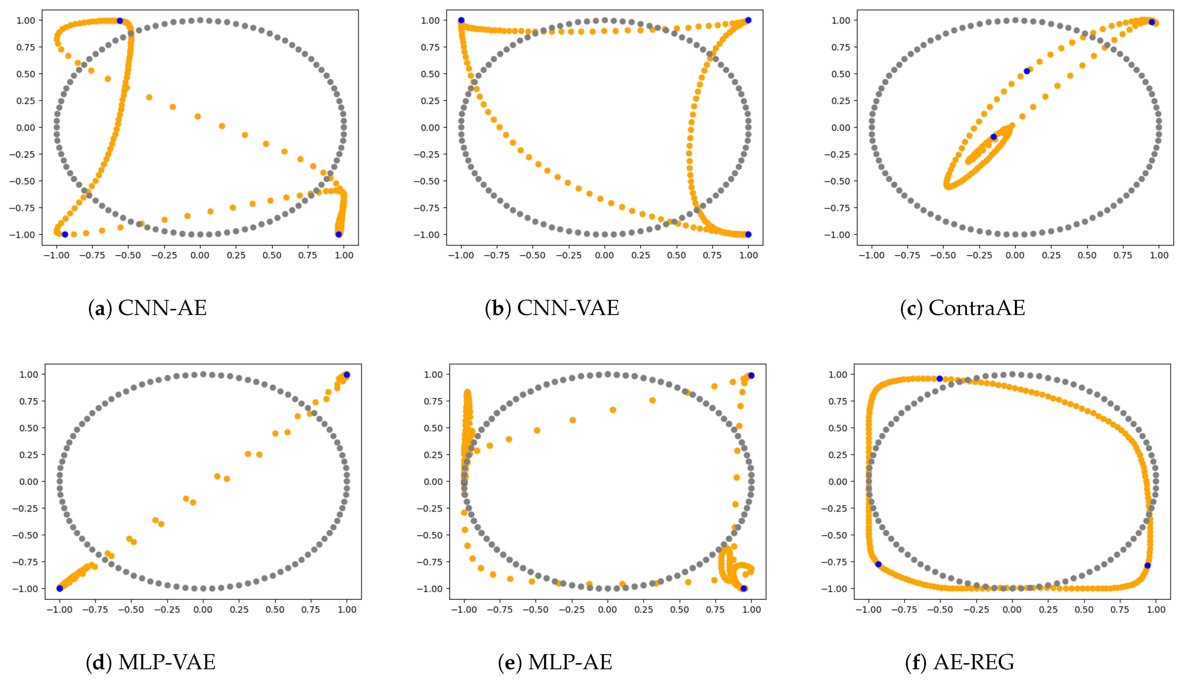
(Cycle reconstructions in dimension 15). We consider the unit circle  S 1 R 2 , a uniform random matrix  A R 15 , 2  with entries in  [ 2 , 2 ]  and the data manifold  D = { A x : x S 1 R 2 } , being an ellipse embedded along some 2-dimensional hyperplane  H A = { A x : x R 2 } R 15 . Due to Bezout’s Theorem [67,68], a 3-points sample uniquely determines a circle in the 2-dimensional plane. Therefore, we executed the AEs for this minimal case of a set of random samples  | D train | = 3 ,  D train D  as training set.
MLP-AE, MLP-VAE, and AE-REG consists of 2 hidden linear layers (in the encoder and decoder), each of length 6. The degree of the Legendre grid P m , n used for the regularization of AE-REG was set to n = 21 , Definition 2. CNN-AE and CNN-VAE consists of 2 hidden convolutional layers with kernel size 3, stride of 2 in the first hidden layer and 1 in the second, and 5 filters per layer. The resulting parameter spaces Υ Ξ 15 , 2 are all of similar size: | Υ Ξ 15 , 2 | 400 . All AEs were trained with the Adam optimizer [69].
Representative results out of 6 repetitions are shown in Figure 2. Only AE-REG delivers a feasible 2D re-embedding, while all other AEs cause overlappings or cycle-crossings. More examples are given in the supplements; whereas AE-REG delivers similar reconstructions for all other trials while the other AEs fail in most of the cases.
Linking back to our initial discussions of ContraAE (R1): The results show that the ambient domain regularization formulated for the ContraAE, is insufficient for guaranteeing a one-to-one encoding. Similarily, CNN-based AEs cause self-intersecting points. As initially discussed in (R3), CNNs are invertible for a generic setup [54], but seem to fail sharply separating tangent T D and perpendicular direction T D of the data manifold D .
We demonstrate the impact of the regularization to not belonging to an edge case by considering the following scenario:
Experiment 2
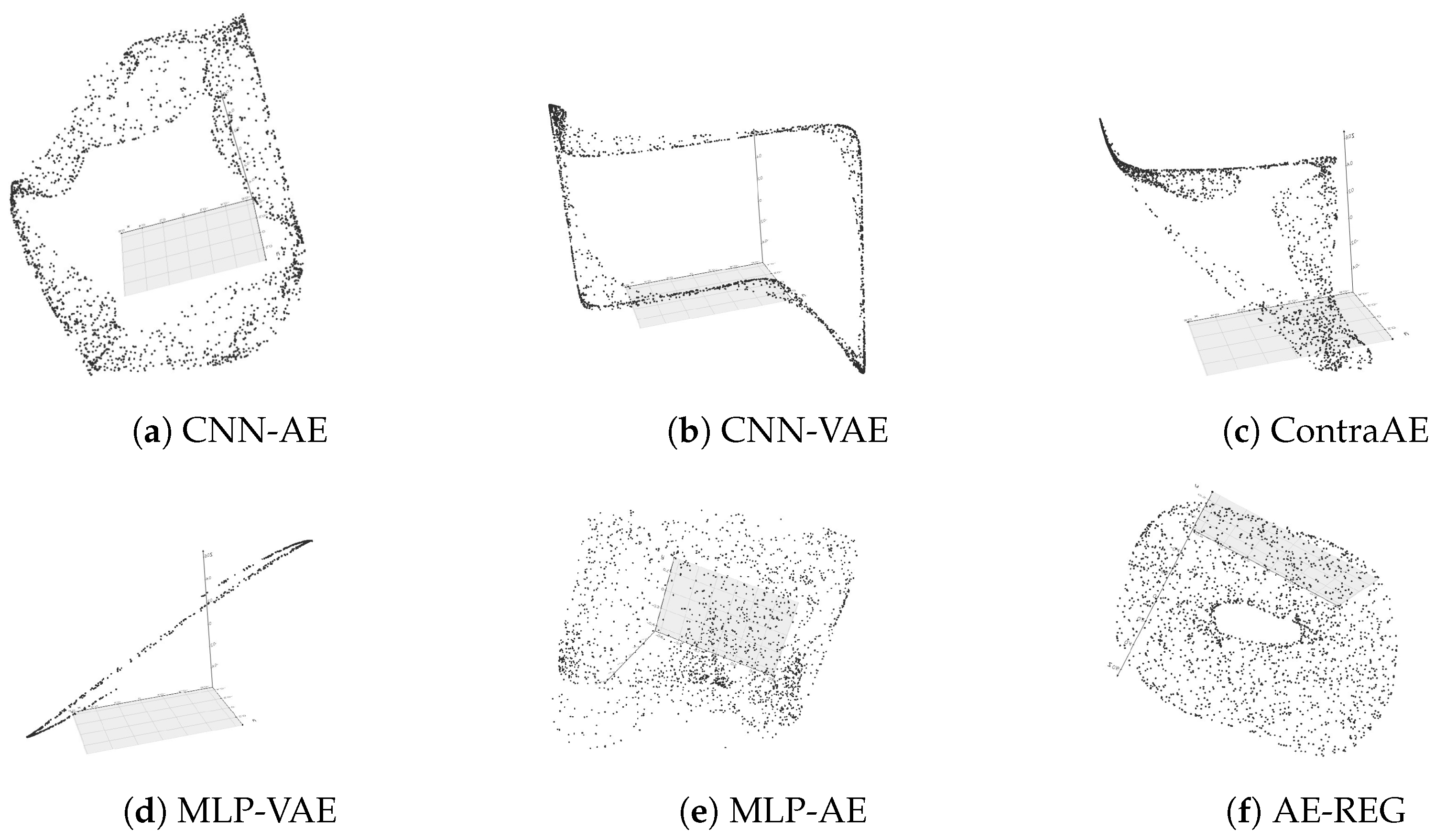
(Torus reconstruction). Following the experimental design of Experiment 1 we generate challenging tori embeddings of a squeezed torus with radii  0 < r , R ,  r = 0.7 R = 2.0  in dimension  m = 15  and dimension  m = 1024  due to multiplication with random matrices  A [ 1 , 1 ] m × 3 . We randomly sample 50 training points  | D train | = 50 ,  D train D  and seek for their 3D re-embedding due to the AEs. We choose a Legendre grid  P m , n  of degree  n = 21 .
A show-case is given in Figure 3, visualized by a dense set of 2000 test points. As in Experiment 1 only AE-REG is capable for re-embedding the torus in a feasible way. MLP-VAE, CNN-AE and CNN-VAE flatten the torus, ContraAE and MPL-AE cause self-intersections. Similar results occur for the high-dimensional case m = 1024 , see the supplements. Summarizing the results suggests that without regularization AE-compression does not preserve the data topology. We continue our evaluation to give further evidence on this expectation.

5.2. Autoencoder Compression for FashionMNIST

We continue by benchmarking on the the classic FashionMNIST dataset [70].
Experiment 3
(FashionMNIST compression). The 70,000 FashionMNIST images separated into 10 fashion classes (T-shirts, shoes, etc.) being of  32 × 32 = 1024 -pixel resolution (ambient domain dimension). For providing a challenging competition, we reduced the dataset to 24,000 uniformly sub-sampled images and trained the AEs for  40 %  training data and complementary test data, respectively. Here, we consider latent dimensions  m = 4 , 10 . Results of further runs for  m = 2 , 4 , 6 , 8 , 10  are given in the supplements.
MLP-AE, MLP-VAE, AE-REG and Hybrid AE-REG consists of 3 hidden layers, each of length 100. The degree of the Legendre grid P m , n used for the regularization of AE-REG was set to n = 21 , Definition 2. CNN-AE and CNN-VAE consists of 3 convolutional layers with kernel size 3, stride of 2. The resulting parameter spaces Υ Ξ 15 , 2 of all AEs are of similar size. Further details of the architectures are reported in the supplements.
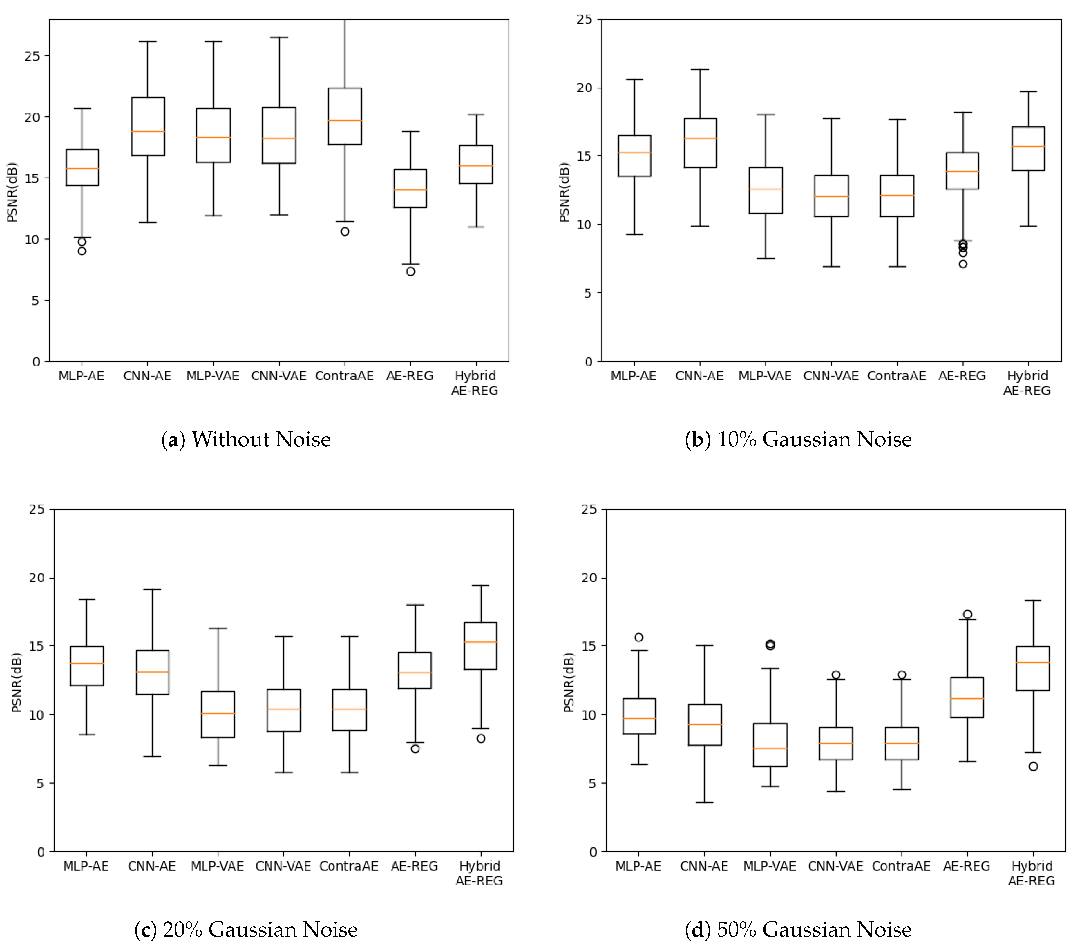
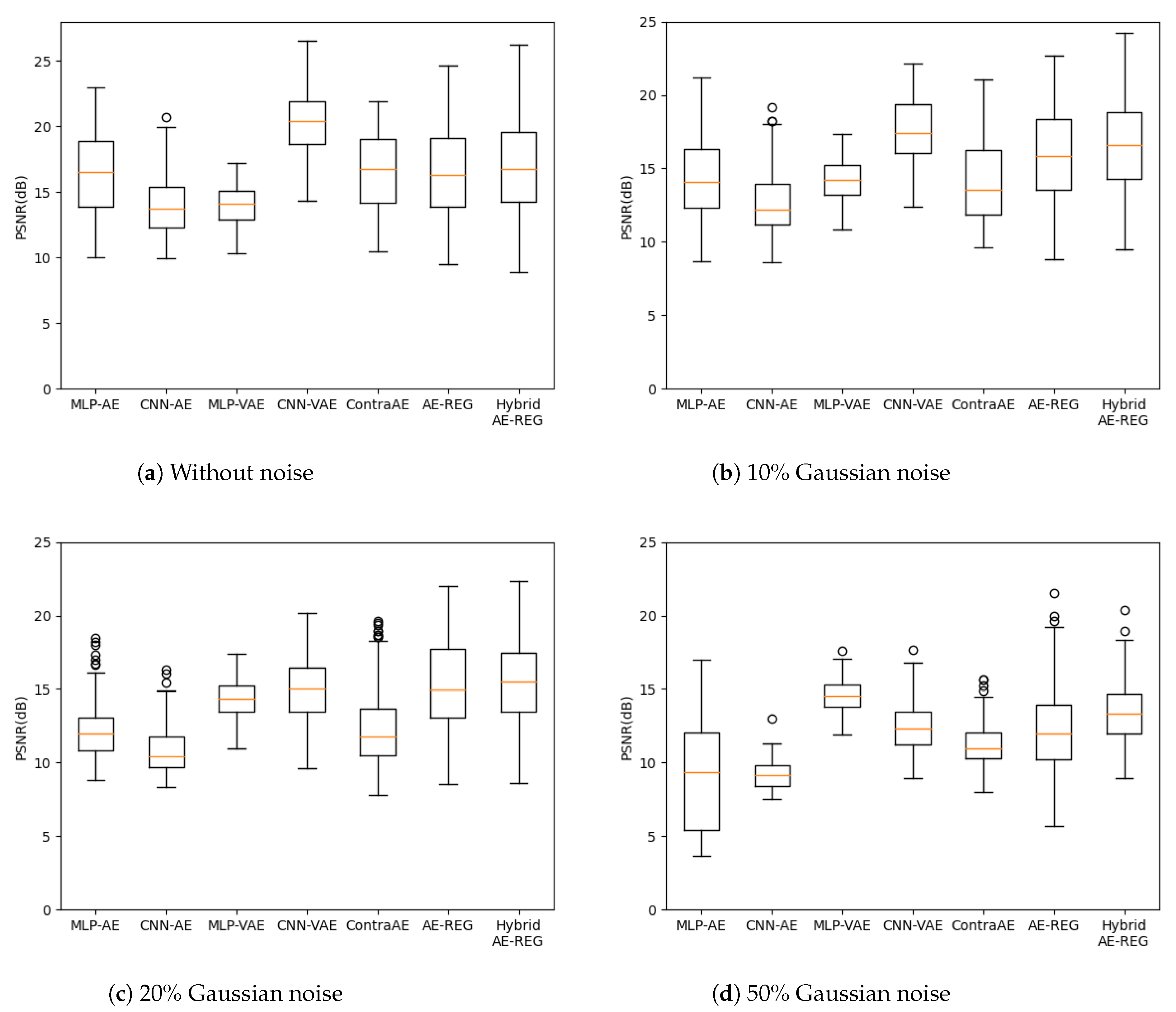
We evaluated the reconstruction quality with respect to peak signal-to-noise ratios (PSNR) for perturbed test data due 0 % , 10 % , 20 % , 50 % of Gaussian noise encoded to latent dimension m = 10 , and plot them in Figure 4. The choice m = 10 , here, reflects the number of FashionMNIST-classes.
While Hybrid AE-REG performs compatible to MLP-AE and worse than the other AEs in the non-perturbed case, its superiority appears already for perturbations with 10 % of Gaussian noise and exceeds the reached reconstruction quality of all other AEs for 20 % Gaussian noise or more. We want to stress that Hybrid AE-REG maintains its reconstruction quality throughout the noise perturbations (up to 70 % , see the supplements). This outstanding appearance of robustness gives strong evidence on the impact of the regularization and well-designed pre-encoding technique due to the hybridization with polynomial regression. Analogue results appear when measuring the reconstruction quality with respect to the structural similarity index measure (SSIM), given in the supplements.
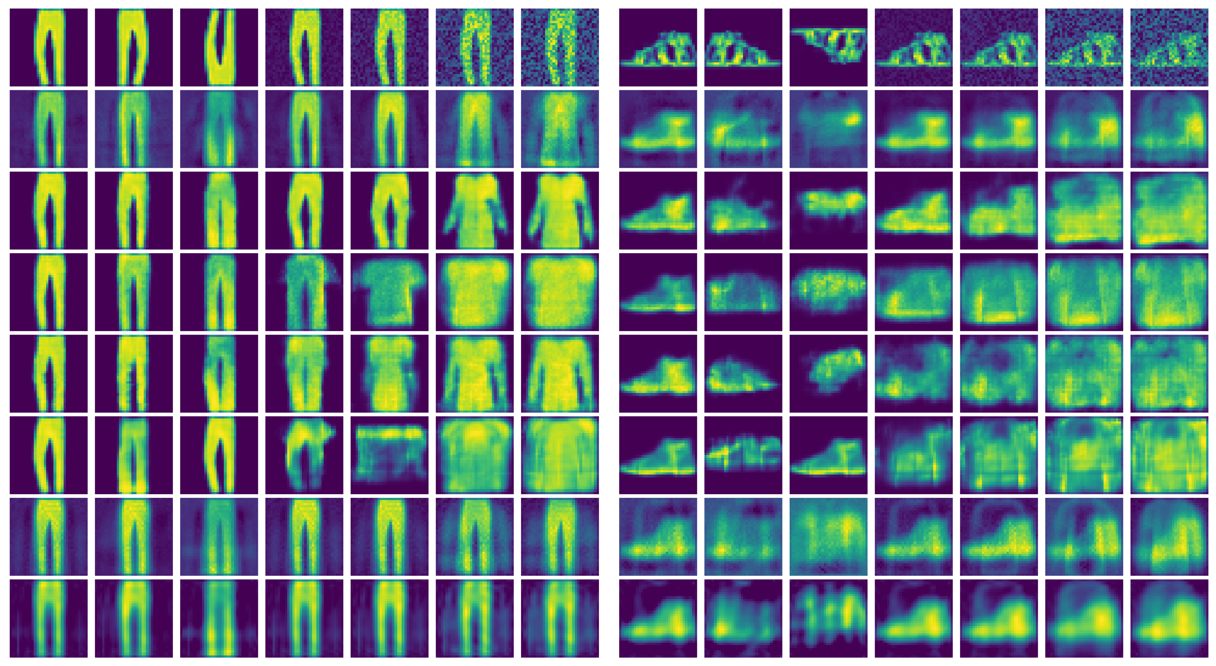
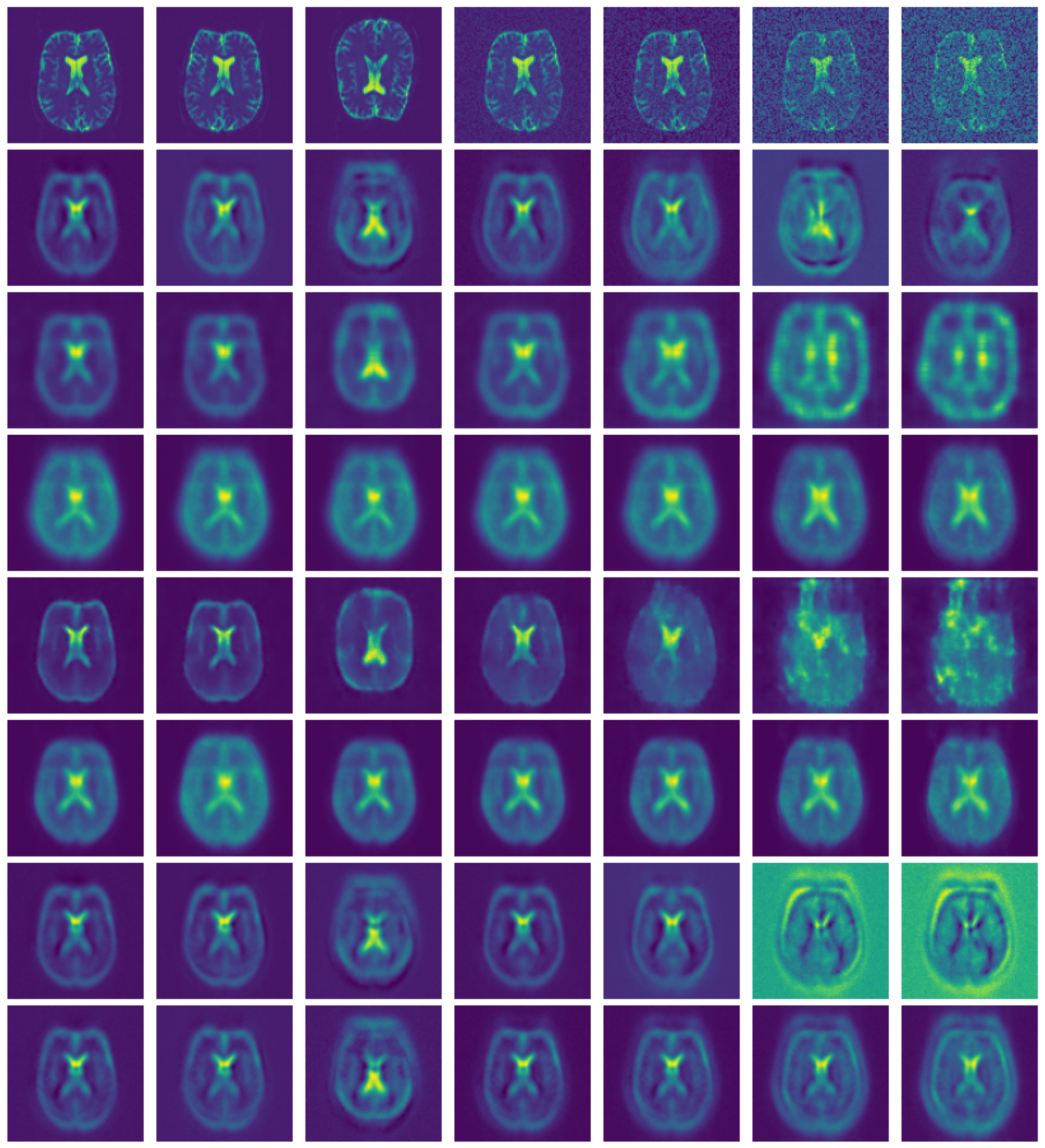
In Figure 5, show cases of the reconstructions are illustrated, including additional vertical and horizontal flip perturbations. Apart from AE-REG and Hybrid AE-REG (rows (7) and (8)), all other AEs flip the FashionMNIST label-class for reconstructions of images with 20 % or 50 % of Gaussian noise. Flipping the label-class is the analogue to topological defects as cycle crossings appeared for the non-regularized AEs in Experiment 1, indicating again that the latent representation of the FashionMNIST dataset given due to the non-regularized AEs does not maintain structural information.
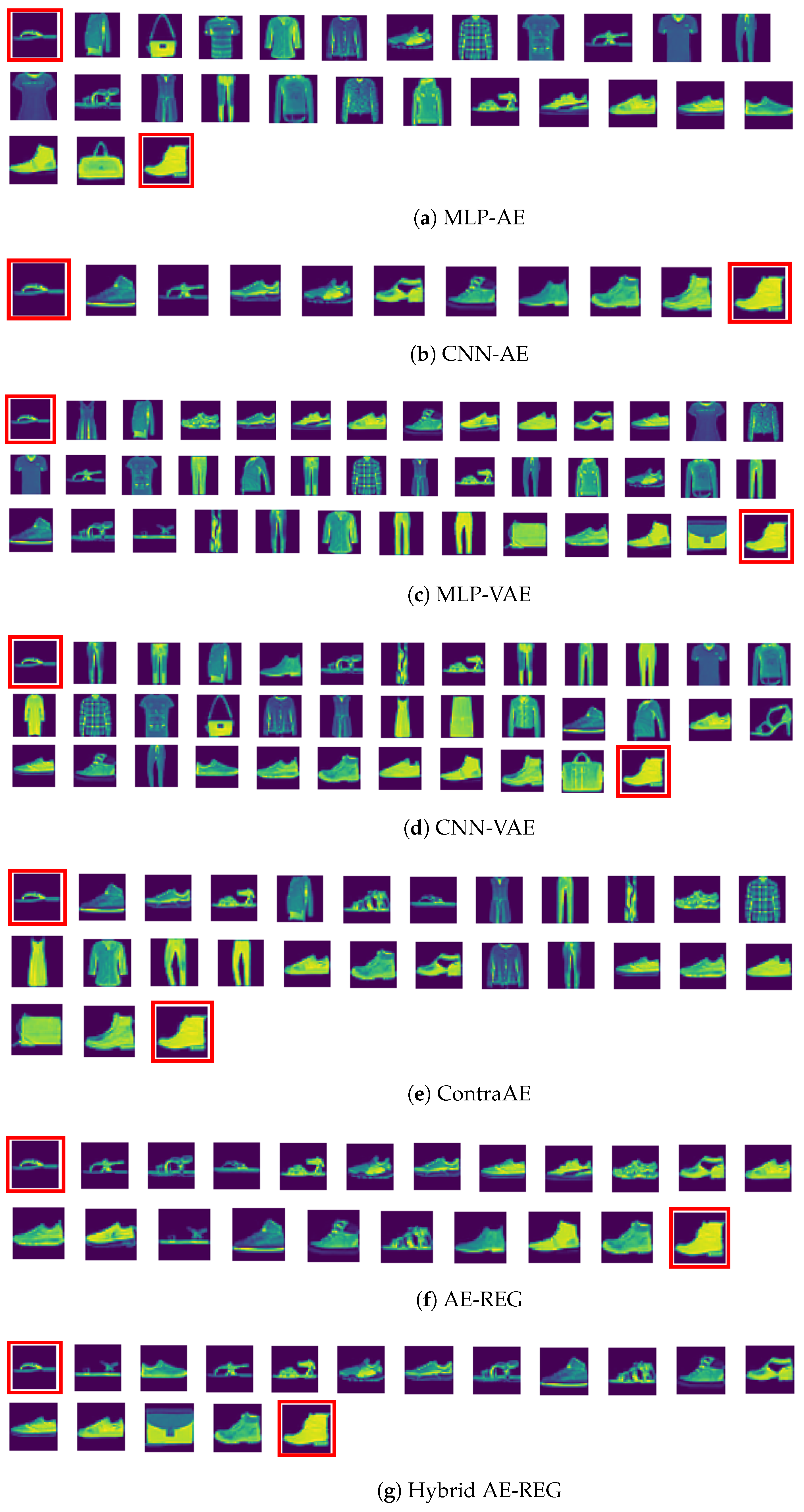
While visualization of the FashionMNIST data manifold is not possible, we decided to investigate its structure by computing geodesics. Figure 6 provides show cases of decoded latent-geodesics ν ( γ ) with respect to latent dimension m = 4 , connecting two AE-latent codes of the encoded test data that has been initially perturbed by 50 % Gaussian noise before encoding. The latent-geodesics γ have to connect the endpoints along the curved encoded data manifold D = φ ( D ) without forbidden short-cuts through D . That is why the geodesics are computed as shortest paths for an early Vietoris–Rips filtration [71] that contains the endpoints in one common connected component. More examples are given in the supplements.
Apart from CNN-AE and AE-REG, all other geodesics contain latent codes of images belonging to another FashionMNIST-class, while for Hybrid AE-REG this happens just once. We interpret these appearances as forbidden short-cuts of ν ( γ ) through D , caused by topological artefacts in D = φ ( D ) .
AE-REG delivers a smoother transition between the endpoints than CNN-AE, suggesting that though the CNN-AE geodesic is shorter, the regularized AEs preserve the topology with higher resolution.

5.3. Autoencoder Compression for Low-Resolution MRI Brain Scans

For evaluating the potential impact of the hybridisation and regularization technique to more realistic high-dimensional problems, we conducted the following experiment.
Experiment 4
(MRI compression). We consider the MRI brain scans dataset from Open Access Series of Imaging Studies (OASIS) [72]. We extract two-dimensional slices from the three-dimensional MRI images, resulting in  60,000  images of resolution  91 × 91 -pixels. We follow Experiment 3 by splitting the dataset into  40 %  training images and complementary test images and compare the AE compression for latent dimension  m = 40 . Results for latent dimension  m = 10 , 15 , 20 , 40 , 60 , 70  and  5 % , 20 % , 40 % , 80 %  training data are given in the supplements, as well as further details on the specifications.
We keep the architecture setup of the AEs, but increase the NN sizes to 5 hidden layers each consisting of 1000 neurons. Reconstructions measured by PSNR are evaluated in Figure 7. Analogous results appear for SSIM, see the supplements.
As in Experiment 3, we observe that AE-REG and Hybrid AE-REG perform compatible or slightly worse than the other AEs in the unperturbed scenario, but show their superiority over the other AEs for 10 % Gaussian noise, or 20 % for CNN-VAE. Hybrid AE-REG specifically maintains its reconstruction quality under noise perturbations up to 20 % (maintains stable for 50 % ). The performance increase compared to the un-regularized MLP-AE becomes evident and validates again that a strong robustness is achieved due to the regularization.
A show case is given in Figure 8. Apart from Hybrid AE-REG (row (8)), all AEs show artefacts when reconstructing perturbed images. CNN-VAE (row (4)) and AE-REG (row (7)) perform compatible and maintain stability up to 20 % Gaussian noise perturbation.
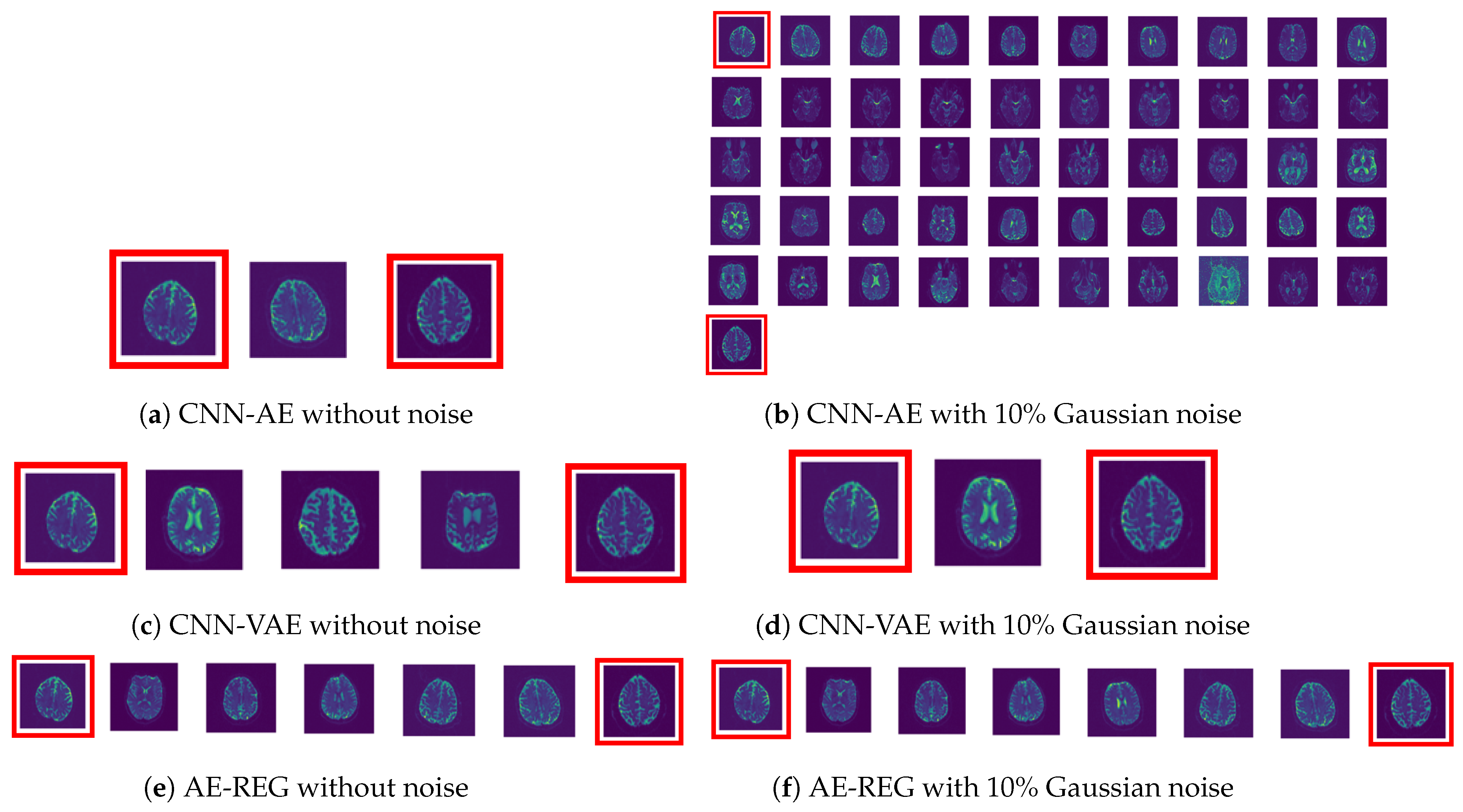
In Figure 9, examples of geodesics are visualized, being computed analogously as in Experiment 3 for the encoded images once without noise and once by adding 10 % Gaussian noise before encoding. The AE-REG geodesic consists of similar slices, including one differing slice for 10 % Gaussian noise perturbation. CNN-VAE delivers a shorter path; however, it includes a strongly differing slice, which is kept for 10 % of Gaussian noise. CNN-AE provides a feasible geodesic in the unperturbed case; however, it becomes unstable in the perturbed case.
We interpret the difference of the AE-REG to CNN-VAE and CNN-AE as an indicator for delivering consistent latent representations on a higher resolution. While the CNN-AE and AE-REG geodesics indicate that one may trust the encoded latent representations, the CNN-AE encoding may not be suitable for reliable post-processing, such as classification tasks. More showcases are given in the supplements, showing similar unstable behaviour of the other AEs.
Summarizing, the results validate once more regularization and hybridization to deliver reliable AEs that are capable for compressing datasets to low-dimensional latent spaces by preserving their topology. A feasible approach to extend the hybridization technique to images or datasets of high resolution is one of the aspects we discuss in our concluding thoughts.

6. Conclusions

We delivered a mathematical theory for addressing encoding tasks of datasets being sampled from smooth data manifolds. Our insights were condensed in an efficiently realizable regularization constraint, resting on sampling the encoder Jacobian in Legendre nodes, located in the latent space. We have proven the regularization to guarantee a re-embedding of the data manifold under mild assumptions on the dataset.
We want to stress that the regularization is not limited to specific NN architectures, but already strongly impacts the performance of simple MLPs. Combinations with initially discussed vectorised AEs [44,45] might extend and improve high-dimensional data analysis as in [9]. When combined with the proposed polynomial regression, the hybridised AEs increase strongly in reconstruction quality. For addressing images of high resolution or multi-dimensional datasets, dim 3 , we propose to apply our recent extension of these regression methods [35].
In summary, the regularized AEs performed far better than the considered alternatives, especially with regard to maintaining the topological structure of the initial dataset. The present computations of geodesics provides a tool for analysing the latent space geometry encoded by the regularized AEs and contributes towards explainability of reliable feature selections, as initially emphasised [13,14,15,16,17].
While structural preservation is substantial for consistent post-analysis, we believe that the proposed regularization technique can deliver new reliable insights across disciplines and may even enable corrections or refinements of prior deduced correlations.

Author Contributions

Conceptualization, M.H.; methodology, C.K.R., J.-E.S.C. and M.H.; software, C.K.R., P.H. and A.W.; validation, C.K.R., P.H., J.-E.S.C. and A.W.; formal analysis, J.-E.S.C. and M.H.; investigation, C.K.R. and A.W.; resources N.H.; data curation, N.H.; writing—original draft preparation, C.K.R. and M.H.; writing—review and editing, M.H.; visualization, C.K.R. and A.W.; supervision, N.H. and M.H. All authors have read and agreed to the published version of the manuscript.

Funding

This work was partially funded by the Center of Advanced Systems Understanding (CASUS), financed by Germany’s Federal Ministry of Education and Research (BMBF) and by the Saxon Ministry for Science, Culture and Tourism (SMWK) with tax funds on the basis of the budget approved by the Saxon State Parliament.

Data Availability Statement

Complete code benchmark sets and supplements are available at https://github.com/casus/autoencoder-regularisation, accessed on 2 June 2024.

Acknowledgments

We express our gratitude to Ivo F. Sbalzarini, Giovanni Volpe, Loic Royer, and Artur Yamimovich for their insightful discussions on autoencoders and their significance in machine learning applications.

Conflicts of Interest

Author Nico Hoffmann was employed by the company SAXONY.ai. The remaining authors declare that the research was conducted in the absence of any commercial or financial relationships that could be construed as a potential conflict of interest.

References

  1. Pepperkok, R.; Ellenberg, J. High-throughput fluorescence microscopy for systems biology. Nat. Rev. Mol. Cell Biol. 2006, 7, 690–696. [Google Scholar] [CrossRef] [PubMed]
  2. Perlman, Z.E.; Slack, M.D.; Feng, Y.; Mitchison, T.J.; Wu, L.F.; Altschuler, S.J. Multidimensional drug profiling by automated microscopy. Science 2004, 306, 1194–1198. [Google Scholar] [CrossRef] [PubMed]
  3. Vogt, N. Machine learning in neuroscience. Nat. Methods 2018, 15, 33. [Google Scholar] [CrossRef]
  4. Carlson, T.; Goddard, E.; Kaplan, D.M.; Klein, C.; Ritchie, J.B. Ghosts in machine learning for cognitive neuroscience: Moving from data to theory. NeuroImage 2018, 180, 88–100. [Google Scholar] [CrossRef] [PubMed]
  5. Zhang, F.; Cetin Karayumak, S.; Hoffmann, N.; Rathi, Y.; Golby, A.J.; O’Donnell, L.J. Deep white matter analysis (DeepWMA): Fast and consistent tractography segmentation. Med. Image Anal. 2020, 65, 101761. [Google Scholar] [CrossRef] [PubMed]
  6. Karniadakis, G.E.; Kevrekidis, I.G.; Lu, L.; Perdikaris, P.; Wang, S.; Yang, L. Physics-informed machine learning. Nat. Rev. Phys. 2021, 3, 422–440. [Google Scholar] [CrossRef]
  7. Rodriguez-Nieva, J.F.; Scheurer, M.S. Identifying topological order through unsupervised machine learning. Nat. Phys. 2019, 15, 790–795. [Google Scholar] [CrossRef]
  8. Willmann, A.; Stiller, P.; Debus, A.; Irman, A.; Pausch, R.; Chang, Y.Y.; Bussmann, M.; Hoffmann, N. Data-Driven Shadowgraph Simulation of a 3D Object. arXiv 2021, arXiv:2106.00317. [Google Scholar]
  9. Kobayashi, H.; Cheveralls, K.C.; Leonetti, M.D.; Royer, L.A. Self-supervised deep learning encodes high-resolution features of protein subcellular localization. Nat. Methods 2022, 19, 995–1003. [Google Scholar] [CrossRef]
  10. Chandrasekaran, S.N.; Ceulemans, H.; Boyd, J.D.; Carpenter, A.E. Image-based profiling for drug discovery: Due for a machine-learning upgrade? Nat. Rev. Drug Discov. 2021, 20, 145–159. [Google Scholar] [CrossRef]
  11. Anitei, M.; Chenna, R.; Czupalla, C.; Esner, M.; Christ, S.; Lenhard, S.; Korn, K.; Meyenhofer, F.; Bickle, M.; Zerial, M.; et al. A high-throughput siRNA screen identifies genes that regulate mannose 6-phosphate receptor trafficking. J. Cell Sci. 2014, 127, 5079–5092. [Google Scholar] [CrossRef]
  12. Nikitina, K.; Segeletz, S.; Kuhn, M.; Kalaidzidis, Y.; Zerial, M. Basic Phenotypes of Endocytic System Recognized by Independent Phenotypes Analysis of a High-throughput Genomic Screen. In Proceedings of the 2019 3rd International Conference on Computational Biology and Bioinformatics, Nagoya, Japan, 17–19 October 2019; pp. 69–75. [Google Scholar]
  13. Ronneberger, O.; Fischer, P.; Brox, T. U-net: Convolutional networks for biomedical image segmentation. In Proceedings of the Medical Image Computing and Computer-Assisted Intervention–MICCAI 2015: 18th International Conference, Munich, Germany, 5–9 October 2015; Proceedings, Part III 18; Springer: Berlin/Heidelberg, Germany, 2015; pp. 234–241. [Google Scholar]
  14. Galimov, E.; Yakimovich, A. A tandem segmentation-classification approach for the localization of morphological predictors of C. elegans lifespan and motility. Aging 2022, 14, 1665. [Google Scholar] [CrossRef]
  15. Yakimovich, A.; Huttunen, M.; Samolej, J.; Clough, B.; Yoshida, N.; Mostowy, S.; Frickel, E.M.; Mercer, J. Mimicry embedding facilitates advanced neural network training for image-based pathogen detection. Msphere 2020, 5, e00836-20. [Google Scholar] [CrossRef] [PubMed]
  16. Fisch, D.; Yakimovich, A.; Clough, B.; Mercer, J.; Frickel, E.M. Image-Based Quantitation of Host Cell–Toxoplasma gondii Interplay Using HRMAn: A Host Response to Microbe Analysis Pipeline. In Toxoplasma gondii: Methods and Protocols; Humana: New York, NY, USA, 2020; pp. 411–433. [Google Scholar]
  17. Andriasyan, V.; Yakimovich, A.; Petkidis, A.; Georgi, F.; Witte, R.; Puntener, D.; Greber, U.F. Microscopy deep learning predicts virus infections and reveals mechanics of lytic-infected cells. Iscience 2021, 24, 102543. [Google Scholar] [CrossRef] [PubMed]
  18. Sánchez, J.; Mardia, K.; Kent, J.; Bibby, J. Multivariate Analysis; Academic Press: London, UK; New York, NY, USA; Toronto, ON, Canada; Sydney, Australia; San Francisco, CA, USA, 1979. [Google Scholar]
  19. Dunteman, G.H. Basic concepts of principal components analysis. In Principal Components Analysis; SAGE Publications Ltd.: London, UK, 1989; pp. 15–22. [Google Scholar]
  20. Krzanowski, W. Principles of Multivariate Analysis; OUP Oxford: Oxford, UK, 2000; Volume 23. [Google Scholar]
  21. Rolinek, M.; Zietlow, D.; Martius, G. Variational Autoencoders Pursue PCA Directions (by Accident). In Proceedings of the 2019 IEEE/CVF Conference on Computer Vision and Pattern Recognition (CVPR), Long Beach, CA, USA, 15–20 June 2019; Volume 2019, pp. 12398–12407. [Google Scholar] [CrossRef]
  22. Antun, V.; Gottschling, N.M.; Hansen, A.C.; Adcock, B. Deep learning in scientific computing: Understanding the instability mystery. SIAM News 2021, 54, 3–5. [Google Scholar]
  23. Gottschling, N.M.; Antun, V.; Adcock, B.; Hansen, A.C. The troublesome kernel: Why deep learning for inverse problems is typically unstable. arXiv 2020, arXiv:2001.01258. [Google Scholar]
  24. Antun, V.; Renna, F.; Poon, C.; Adcock, B.; Hansen, A.C. On instabilities of deep learning in image reconstruction and the potential costs of AI. Proc. Natl. Acad. Sci. USA 2020, 117, 30088–30095. [Google Scholar] [CrossRef]
  25. Chen, H.; Zhang, H.; Si, S.; Li, Y.; Boning, D.; Hsieh, C.J. Robustness Verification of Tree-based Models. In Proceedings of the Advances in Neural Information Processing Systems; Wallach, H., Larochelle, H., Beygelzimer, A., d’Alché-Buc, F., Fox, E., Garnett, R., Eds.; Curran Associates, Inc.: Red Hook, NY, USA, 2019; Volume 32. [Google Scholar]
  26. Galhotra, S.; Brun, Y.; Meliou, A. Fairness testing: Testing software for discrimination. In Proceedings of the 2017 11th Joint Meeting on Foundations of Software Engineering, Paderborn, Germany, 4–8 September 2017; pp. 498–510. [Google Scholar]
  27. Mazzucato, D.; Urban, C. Reduced products of abstract domains for fairness certification of neural networks. In Proceedings of the Static Analysis: 28th International Symposium, SAS 2021, Chicago, IL, USA, 17–19 October 2021; Proceedings 28; Springer: Berlin/Heidelberg, Germany, 2021; pp. 308–322. [Google Scholar]
  28. Lang, S. Differential Manifolds; Springer: Berlin/Heidelberg, Germany, 1985. [Google Scholar]
  29. Krantz, S.G.; Parks, H.R. The implicit function theorem. Modern Birkhäuser Classics. In History, Theory, and Applications, 2003rd ed.; Birkhäuser/Springer: New York, NY, USA, 2013; Volume 163, p. xiv. [Google Scholar]
  30. Stroud, A. Approximate Calculation of Multiple Integrals: Prentice-Hall Series in Automatic Computation; Prentice-Hall: Englewood, NJ, USA, 1971. [Google Scholar]
  31. Stroud, A.; Secrest, D. Gaussian Quadrature Formulas; Prentice-Hall: Englewood, NJ, USA, 2011. [Google Scholar]
  32. Trefethen, L.N. Multivariate polynomial approximation in the hypercube. Proc. Am. Math. Soc. 2017, 145, 4837–4844. [Google Scholar] [CrossRef]
  33. Trefethen, L.N. Approximation Theory and Approximation Practice; SIAM: Philadelphia, PA, USA, 2019; Volume 164. [Google Scholar]
  34. Sobolev, S.L.; Vaskevich, V. The Theory of Cubature Formulas; Springer Science & Business Media: Berlin/Heidelberg, Germany, 1997; Volume 415. [Google Scholar]
  35. Veettil, S.K.T.; Zheng, Y.; Acosta, U.H.; Wicaksono, D.; Hecht, M. Multivariate Polynomial Regression of Euclidean Degree Extends the Stability for Fast Approximations of Trefethen Functions. arXiv 2022, arXiv:2212.11706. [Google Scholar]
  36. Suarez Cardona, J.E.; Hofmann, P.A.; Hecht, M. Learning Partial Differential Equations by Spectral Approximates of General Sobolev Spaces. arXiv 2023, arXiv:2301.04887. [Google Scholar]
  37. Suarez Cardona, J.E.; Hecht, M. Replacing Automatic Differentiation by Sobolev Cubatures fastens Physics Informed Neural Nets and strengthens their Approximation Power. arXiv 2022, arXiv:2211.15443. [Google Scholar]
  38. Hecht, M.; Cheeseman, B.L.; Hoffmann, K.B.; Sbalzarini, I.F. A Quadratic-Time Algorithm for General Multivariate Polynomial Interpolation. arXiv 2017, arXiv:1710.10846. [Google Scholar]
  39. Hecht, M.; Hoffmann, K.B.; Cheeseman, B.L.; Sbalzarini, I.F. Multivariate Newton Interpolation. arXiv 2018, arXiv:1812.04256. [Google Scholar]
  40. Hecht, M.; Gonciarz, K.; Michelfeit, J.; Sivkin, V.; Sbalzarini, I.F. Multivariate Interpolation in Unisolvent Nodes–Lifting the Curse of Dimensionality. arXiv 2020, arXiv:2010.10824. [Google Scholar]
  41. Hecht, M.; Sbalzarini, I.F. Fast Interpolation and Fourier Transform in High-Dimensional Spaces. In Proceedings of the Intelligent Computing; Arai, K., Kapoor, S., Bhatia, R., Eds.; Advances in Intelligent Systems and Computing; Springer International Publishing: Cham, Switzerland, 2018; Volume 857, pp. 53–75. [Google Scholar]
  42. Sindhu Meena, K.; Suriya, S. A Survey on Supervised and Unsupervised Learning Techniques. In Proceedings of the International Conference on Artificial Intelligence, Smart Grid and Smart City Applications; Kumar, L.A., Jayashree, L.S., Manimegalai, R., Eds.; Springer International Publishing: Cham, Switzerland, 2020; pp. 627–644. [Google Scholar]
  43. Chao, G.; Luo, Y.; Ding, W. Recent Advances in Supervised Dimension Reduction: A Survey. Mach. Learn. Knowl. Extr. 2019, 1, 341–358. [Google Scholar] [CrossRef]
  44. Mitchell, T.M. The Need for Biases in Learning Generalizations; Citeseer: Berkeley, CA, USA, 1980. [Google Scholar]
  45. Gordon, D.F.; Desjardins, M. Evaluation and selection of biases in machine learning. Mach. Learn. 1995, 20, 5–22. [Google Scholar] [CrossRef]
  46. Wu, H.; Flierl, M. Vector quantization-based regularization for autoencoders. In Proceedings of the AAAI Conference on Artificial Intelligence, New York, NY, USA, 7–12 February 2020; Volume 34, pp. 6380–6387. [Google Scholar]
  47. Van Den Oord, A.; Vinyals, O.; Kavukcuoglu, K. Neural discrete representation learning. Adv. Neural Inf. Process. Syst. 2017, 30, 6306–6315. [Google Scholar]
  48. Rifai, S.; Mesnil, G.; Vincent, P.; Muller, X.; Bengio, Y.; Dauphin, Y.; Glorot, X. Higher order contractive auto-encoder. In Proceedings of the Joint European Conference on Machine Learning and Knowledge Discovery in Databases, Athens, Greece, 5–9 September 2011; Springer: Berlin/Heidelberg, Germany, 2011; pp. 645–660. [Google Scholar]
  49. Rifai, S.; Vincent, P.; Muller, X.; Glorot, X.; Bengio, Y. Contractive auto-encoders: Explicit invariance during feature extraction. In Proceedings of the 28th International Conference on International Conference on Machine Learning (ICML), Bellevue, WA, USA, 28 June–2 July 2011. [Google Scholar]
  50. Kingma, D.P.; Welling, M. Auto-encoding variational bayes. arXiv 2013, arXiv:1312.6114. [Google Scholar]
  51. Burgess, C.P.; Higgins, I.; Pal, A.; Matthey, L.; Watters, N.; Desjardins, G.; Lerchner, A. Understanding disentangling in β-VAE. arXiv 2018, arXiv:1804.03599. [Google Scholar]
  52. Kumar, A.; Poole, B. On implicit regularization in β-VAEs. In Proceedings of the 37th International Conference on Machine Learning (ICML 2020), Vienna, Austria, 12–18 July 2020; pp. 5436–5446. [Google Scholar]
  53. Rhodes, T.; Lee, D. Local Disentanglement in Variational Auto-Encoders Using Jacobian L_1 Regularization. Adv. Neural Inf. Process. Syst. 2021, 34, 22708–22719. [Google Scholar]
  54. Gilbert, A.C.; Zhang, Y.; Lee, K.; Zhang, Y.; Lee, H. Towards understanding the invertibility of convolutional neural networks. In Proceedings of the 26th International Joint Conference on Artificial Intelligence, Melbourne, Australia, 19–25 August 2017; pp. 1703–1710. [Google Scholar]
  55. Anthony, M.; Bartlett, P.L. Neural Network Learning: Theoretical Foundations; Cambridge University Press: Cambridge, MA, USA, 2009. [Google Scholar]
  56. Goodfellow, I.; Bengio, Y.; Courville, A. Deep Learning; MIT Press: Cambridge, MA, USA, 2016. [Google Scholar]
  57. Adams, R.A.; Fournier, J.J. Sobolev Spaces; Academic Press: Cambridge, MA, USA, 2003; Volume 140. [Google Scholar]
  58. Brezis, H. Functional Analysis, Sobolev Spaces and Partial Differential Equations; Springer: Berlin/Heidelberg, Germany, 2011; Volume 2. [Google Scholar]
  59. Pedersen, M. Functional Analysis in Applied Mathematics and Engineering; CRC Press: Boca Raton, FL, USA, 2018. [Google Scholar]
  60. Gautschi, W. Numerical Analysis; Springer Science & Business Media: Berlin/Heidelberg, Germany, 2011. [Google Scholar]
  61. Chen, W.; Chern, S.S.; Lam, K.S. Lectures on Differential Geometry; World Scientific Publishing Company: Singapore, 1999; Volume 1. [Google Scholar]
  62. Taubes, C.H. Differential Geometry: Bundles, Connections, Metrics and Curvature; OUP Oxford: Oxford, UK, 2011; Volume 23. [Google Scholar]
  63. Do Carmo, M.P. Differential Geometry of Curves and Surfaces: Revised and Updated, 2nd ed.; Courier Dover Publications: Mineola, NY, USA, 2016. [Google Scholar]
  64. Weierstrass, K. Über die analytische Darstellbarkeit sogenannter willkürlicher Funktionen einer reellen Veränderlichen. Sitzungsberichte K. Preußischen Akad. Wiss. Berl. 1885, 2, 633–639. [Google Scholar]
  65. De Branges, L. The Stone-Weierstrass Theorem. Proc. Am. Math. Soc. 1959, 10, 822–824. [Google Scholar] [CrossRef]
  66. Baydin, A.G.; Pearlmutter, B.A.; Radul, A.A.; Siskind, J.M. Automatic differentiation in machine learning: A survey. J. Mach. Learn. Res. 2018, 18, 1–43. [Google Scholar]
  67. Bézout, E. Théorie Générale des Équations Algébriques; de l’imprimerie de Ph.-D. Pierres: Paris, France, 1779. [Google Scholar]
  68. Fulton, W. Algebraic Curves (Mathematics Lecture Note Series); The Benjamin/Cummings Publishing Co., Inc.: Menlo Park, CA, USA, 1974. [Google Scholar]
  69. Kingma, D.P.; Ba, J. Adam: A method for stochastic optimization. arXiv 2014, arXiv:1412.6980. [Google Scholar]
  70. Xiao, H.; Rasul, K.; Vollgraf, R. Fashion-MNIST: A Novel Image Dataset for Benchmarking Machine Learning Algorithms. arXiv 2017, arXiv:1708.07747. [Google Scholar]
  71. Moor, M.; Horn, M.; Rieck, B.; Borgwardt, K. Topological autoencoders. In Proceedings of the International Conference on Machine Learning, Virtual, 13–18 July 2020; pp. 7045–7054. [Google Scholar]
  72. Marcus, D.S.; Wang, T.H.; Parker, J.; Csernansky, J.G.; Morris, J.C.; Buckner, R.L. Open Access Series of Imaging Studies (OASIS): Cross-sectional MRI data in young, middle aged, nondemented, and demented older adults. J. Cogn. Neurosci. 2007, 19, 1498–1507. [Google Scholar] [CrossRef]
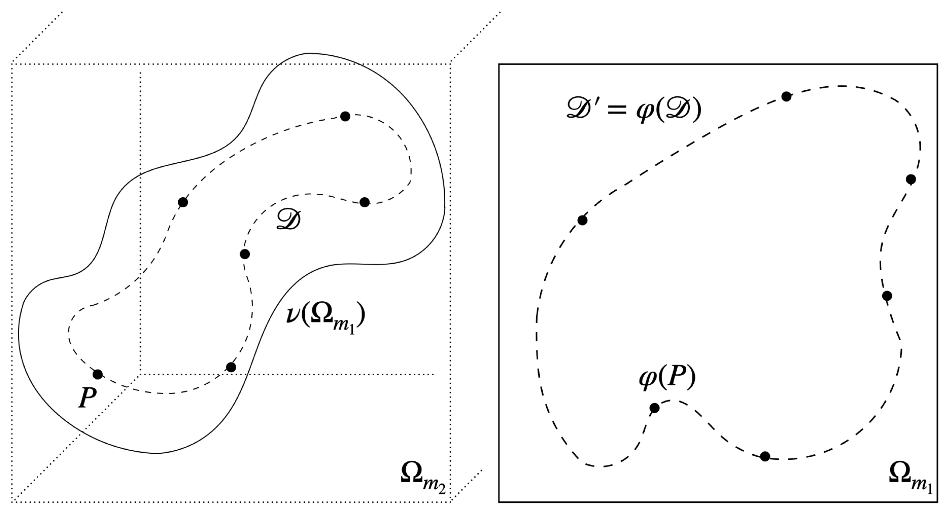
Figure 1. Illustration of the latent representation D = φ ( D ) Ω m 1 of the data manifold D Ω m 2 , dim D = m 0 < m 1 < m 2 N given by the autoencoder ( φ , ν ) . The decoder is a one-to-one mapping of the hypercube Ω m 1 to its image ν ( Ω m 1 ) D , including D in its interior and consequently guaranteeing Equation (1).
Axioms 13 00535 g001
Figure 2. Circle reconstruction using various autoencoder models.
Axioms 13 00535 g002
Figure 3. Torus reconstruction using various autoencoder models, dim = 15 .
Axioms 13 00535 g003
Figure 4. FashionMNIST reconstruction with varying levels of Gaussian noise, latent dimension dim = 10 .
Axioms 13 00535 g004
Figure 5. Two show cases of FashionMNIST reconstruction for latent dimension m = 10 . First row shows the input image with vertical, horizontal flips, and 0 % , 10 % , 20 % , 50 % , 70 % of Gaussian noise. Rows beneath show the results of (2) MLAP-AE, (3) CNN-AE, (4) MLP-VAE, (5) CNN-VAE, (6) ContraAE, (7) AE-REG, and (8) Hybrid AE-REG.
Axioms 13 00535 g005
Figure 6. FashionMNIST geodesics in latent dimension dim = 4 .
Axioms 13 00535 g006
Figure 7. MRI reconstruction, latent dimension dim = 40 .
Axioms 13 00535 g007
Figure 8. MRI show case. First row shows the input image with vertical, horizontal flips, and 0 % , 10 % , 20 % , 50 % , 70 % of Gaussian noise. Rows beneath show the results of (2) MLAP-AE, (3) CNN-AE, (4) MLP-VAE, (5) CNN-VAE, (6) ContraAE, (7) AE-REG, and (8) Hybrid AE-REG.
Axioms 13 00535 g008
Figure 9. MRI geodesics for latent dimension dim = 40 with various levels of Gaussian noise.
Axioms 13 00535 g009
Disclaimer/Publisher’s Note: The statements, opinions and data contained in all publications are solely those of the individual author(s) and contributor(s) and not of MDPI and/or the editor(s). MDPI and/or the editor(s) disclaim responsibility for any injury to people or property resulting from any ideas, methods, instructions or products referred to in the content.