Some Statistical and Direct Approximation Properties for a New Form of the Generalization of q-Bernstein Operators with the Parameter λ

Abstract

In this study, a different generalization of q-Bernstein operators with the parameter $\lambda \in [-1,1]$ is created. The moments and central moments of these operators are calculated, a statistical approximation result for this new type of $(\lambda ,q)$-Bernstein operators is obtained, and the convergence properties are analyzed using the Peetre K-functional and the modulus of continuity for this new operator. Finally, a numerical example is given to illustrate the convergence behavior of the newly defined operators.

1. Introduction

The well-known way to find a new function approximating a function is to use Bernstein operators, where the function is a continuous function defined on the interval $[0,1]$. Over the years, researchers have developed several variations of this operator, sometimes expanding the function space studied (for example, eliminating the necessity for the function to be continuous), sometimes extending the domain of the function, and sometimes achieving a better approximation rate, even though working in the same function space. Especially in recent years, there have been many examples (see [1,2,3,4,5,6,7,8,9]).

In our paper, we focus on a generalization of the q-analogue of Bernstein operators, because studying the area of q-calculus is very important, as it has many applications in mathematics, mechanics, and physics. In the area of approximation theory, the pioneering researcher who brought the q-analogue of Bernstein polynomials to the literature was Professor Lupaş (see [10]). After a decade, another generalization of q-Bernstein polynomials was presented by Phillips [11]. Many years later, q-Bernstein operators were studied [12,13,14]. Following these developments, many researchers have investigated the approximation properties of various types of q-Bernstein operators by further developing this type of operator (see [15,16,17,18,19,20,21,22,23]). Furthermore, not only the q-analogues of the Bernstein operators but also the q-analogues of various other operators have been extensively studied (see [24,25,26,27,28,29,30,31,32,33]), which indicates how productive these studies on q-analysis are.

Another important issue is the use of Bernstein polynomial bases with certain properties to create surfaces and curves in computer-aided geometric design (CAGD) (see [34,35,36]) and computer graphics. An important and comprehensive study explaining this subject was conducted by Farouki [37]. These basis functions are effective in the numerical solutions of partial differential equations, CAGD, font design, and 3D modeling.

Before mentioning the other studies motivating us, it is necessary to explain the new concepts used in such studies, in other words, the q-analogues of the ordinary definitions, so that it is easy to understand what was achieved in these inspiring studies. Therefore, we start by explaining these. Firstly, we elucidate q-integers. For further details about q-integers, we refer the interested reader to references [38,39].

Let a value $q>0$ be given and s be a non-negative integer. The q-integer ${\left[s\right]}_q$ is defined by

$${\left[s\right]}_q:=\left\{\begin{array}{cc}{\displaystyle \frac{1-q^s}{1-q}},\hfill & \mathrm{if}q\ne 1,\hfill \\ s,\hfill & \mathrm{if}q=1.\hfill \end{array}\right.$$

In addition to that, the q-factorial is expressed as

$${\left[s\right]}_q!:=\left\{\begin{array}{cc}{\left[s\right]}_q{[s-1]}_q\cdots {\left[1\right]}_q,\hfill & \mathrm{if}s=1,2,\cdots ,\hfill \\ 1,\hfill & \mathrm{if}s=0,\hfill \end{array}\right.$$

and q-binomial coefficients are also defined as

$${\left[\begin{array}{c}v\\ s\end{array}\right]}_q:={\displaystyle \frac{{\left[v\right]}_q!}{{[v-s]}_q!{\left[s\right]}_q!}}\mathrm{for}0\le s\le v.$$

From now on, we assume that $q\in \left(\left.0,1\right]\right.$ throughout entire study. At this stage, we can now introduce the studies that form a cornerstone for us. Let us mention q-Bernstein operators. Suppose that h is a continuous function defined on $[0,1]$, the q-Bernstein operators introduced by Phillips [11] are in the following form:

$$B_{v,q}(h;x)=\sum _{s=0}^v{b}_{v,s}(x;q)h\left({\displaystyle \frac{{\left[s\right]}_q}{{\left[v\right]}_q}}\right),$$

(1)

where $b_{v,s}(x;q)(s=0,1,\cdots ,v)$ are the basis functions of q-Bernstein operators. Before providing the definition of $b_{v,s}(x;q)$, we need to decide which notation to use instead of ${\prod }_{r=0}^{v-s-1}(1-q^{r}x)$. From now on, we will presume that ${\prod }_{r=0}^{v-s-1}(1-q^{r}x)={(1⊝x)}^{v-s}$ for simplicity and brevity. Now, we present the definition of $b_{v,s}(x,q)$ as follows:

$$b_{v,s}(x;q)={\left[\begin{array}{c}v\\ s\end{array}\right]}_q{x}^s\prod _{r=0}^{v-s-1}(1-q^{r}x)={\left[\begin{array}{c}v\\ s\end{array}\right]}_q{x}^s{(1⊝x)}^{v-s}.$$

(2)

Let $-1\le \lambda \le 1$, $x\in [0,1]$ and $0<q\le 1$. Inspired by the above studies, under these assumptions, we establish $(\lambda ,q)$-Bernstein operators defined as follows:

$$B_{v,q}^{\lambda }(h;x)=\sum _{s=0}^v{b}_{v,s}^{\lambda }(x;q)h\left({\displaystyle \frac{{\left[s\right]}_q}{{\left[v\right]}_q}}\right),$$

(3)

where

$$\left\{\begin{array}{c}\begin{array}{cc}\hfill b_{v,0}^{\lambda }(x;q)& =b_{v,0}(x;q)-{\displaystyle \frac{\lambda }{{\left[v\right]}_q+1}}{b}_{v+1,1}(x;q);\hfill \\ \hfill b_{v,s}^{\lambda }(x;q)& =b_{v,s}(x;q)+{\displaystyle \frac{\lambda }{{\left[v\right]}_q+1}}\left(b_{v+1,s}(x;q)-b_{v+1,s+1}(x;q)\right);(s=1,2,\cdots ,v-1)\hfill \\ \hfill b_{v,v}^{\lambda }(x;q)& =b_{v,v}(x;q)+{\displaystyle \frac{\lambda }{{\left[v\right]}_q+1}}{b}_{v+1,v}(x;q),\hfill \end{array}\hfill \end{array}\right.$$

In addition, $b_{v,s}(x;q)$ are defined in (2) and h is a continuous function on $[0,1]$.

Firstly, it is clear that the operators $B_{v,q}^0(h;x)$ reduce to the q-Bernstein operators given in (1) when $\lambda =0$; moreover, the operators $B_{v,1}^0(h;x)$ transform into well-known classical Bernstein operators when $\lambda =0,q=1$. Secondly, if $q=1$, the operators $B_{v,1}^{\lambda }(h;x)$ convert into the $\lambda$-Bernstein operators introduced in [40].

In this study, we present statistical approximation results using the notion of statistical convergence for a new generalization of q-Bernstein operators with the parameter $\lambda$. After this stage, we give the convergence properties thanks to the Peetre K-functional for this operator. To achieve this, we first establish several lemmas that play a crucial role in our main results.

2. Auxiliary Results

The lemmas we use in the proof of the main results are as follows:

Lemma 1.

Let $-1\le \lambda \le 1$, $x\in [0,1]$, and $0<q\le 1$. Then, the operators $B_{v,q}^{\lambda }(h;x)$ are positive linear operators.

Proof. 

It is obvious that the operators $B_{v,q}^{\lambda }\left(h\right)$ are linear, so it is sufficient that we prove these operators to be positive, i.e., $b_{v,s}^{\lambda }(x;q)\ge 0$ for $0\le s\le v$.

It is worth noting that the inequality

$$b_{v,s}(x;q)\ge 0$$

(4)

holds for $s=0,1,\cdots ,v$, as demonstrated in [11].

For $s=0$, utilizing ${[v+1]}_q\le {\left[v\right]}_q+1$ and the inequality stated in (4), we obtain

$$\begin{array}{cc}\hfill b_{v,0}^{\lambda }(x;q)& =b_{v,0}(x;q)-{\displaystyle \frac{\lambda }{{\left[v\right]}_q+1}}{b}_{v+1,1}(x;q)\hfill \\ & =b_{v,0}(x;q)\left(1-{\displaystyle \frac{{[v+1]}_q}{{\left[v\right]}_q+1}}\lambda x\right)\ge 0.\hfill \end{array}$$

For $s=v$, we have

$$\begin{array}{cc}\hfill b_{v,v}^{\lambda }(x;q)& =b_{v,v}(x;q)+{\displaystyle \frac{\lambda }{{\left[v\right]}_q+1}}{b}_{v+1,v}(x;q)\hfill \\ & =b_{v,v}(x;q)\left(1+{\displaystyle \frac{\lambda {[v+1]}_q}{{\left[v\right]}_q+1}}(1-x)\right)\ge 0,\hfill \end{array}$$

because $0<{\displaystyle \frac{{[v+1]}_q}{{\left[v\right]}_q+1}}\le 1$, $0\le 1-x\le 1$, and $\lambda \in [-1,1]$.

First of all, since $0\le {\displaystyle \frac{(1-q^{v-s}x)}{{[v+1-s]}_q}}\le {\displaystyle \frac{1}{{\left[2\right]}_q}}$ and $-{\displaystyle \frac{1}{{\left[2\right]}_q}}\le -{\displaystyle \frac{x}{{[s+1]}_q}}\le 0$ for $1\le s\le v-1$, we establish the following inequality:

$$-1<{\displaystyle \frac{(1-q^{v-s}x)}{{[v+1-s]}_q}}-{\displaystyle \frac{x}{{[s+1]}_q}}<1.$$

(5)

We obtain

$$\begin{array}{cc}\hfill b_{v,s}^{\lambda }(x;q)& =b_{v,s}(x;q)+{\displaystyle \frac{\lambda }{{\left[v\right]}_q+1}}\left(b_{v+1,s}(x;q)-b_{v+1,s+1}(x;q)\right)\hfill \\ & =b_{v,s}(x;q)\left(1+{\displaystyle \frac{\lambda {[v+1]}_q}{{\left[v\right]}_q+1}}\left({\displaystyle \frac{(1-q^{v-s}x)}{{[v+1-s]}_q}}-{\displaystyle \frac{x}{{[s+1]}_q}}\right)\right)\ge 0\hfill \end{array}$$

by considering the inequalities given in (4) and (5).

As a result, we obtain the proof. □

Lemma 2.

Let $x\in [0,1]$, $0<q\le 1$ and $\lambda \in [-1,1]$. For the $(\lambda ,q)$-Bernstein operators $B_{v,q}^{\lambda }(h;x)$$(v>0)$, the following equalities hold:

$$\begin{array}{cc}\hfill B_{v,q}^{\lambda }(1;x)=& 1,\hfill \end{array}$$

(6)

$$\begin{array}{cc}\hfill B_{v,q}^{\lambda }(t;x)=& x+{\displaystyle \frac{\lambda (q-1){[v+1]}_q}{({\left[v\right]}_q+1)q{\left[v\right]}_q}}x(1-x^v)+{\displaystyle \frac{\lambda }{({\left[v\right]}_q+1)q{\left[v\right]}_q}}(1-x^{v+1}-{(1⊝x)}^{v+1})\hfill \end{array}$$

(7)

$$\begin{array}{cc}\hfill B_{v,q}^{\lambda }(t^2;x)=& x^2+{\displaystyle \frac{x(1-x)}{{\left[v\right]}_q}}+{\displaystyle \frac{\lambda (q^2+1){[v+1]}_q}{({\left[v\right]}_q+1)q^2{\left[v\right]}_q^2}}x(1-x^v)\hfill \\ \hfill & +{\displaystyle \frac{\lambda (q^2-1){[v+1]}_q}{({\left[v\right]}_q+1)q{\left[v\right]}_q}}{x}^2(1-x^{v-1})-{\displaystyle \frac{\lambda }{({\left[v\right]}_q+1)q^2{\left[v\right]}_q^2}}(1-x^{v+1}-{(1⊝x)}^{v+1}).\hfill \end{array}$$

(8)

Proof. 

If we perform some straightforward mathematical calculations, we conclude that

$$B_{v,q}^{\lambda }(h;x)=\sum _{s=0}^v{b}_{v,s}(x;q)h\left({\displaystyle \frac{{\left[s\right]}_q}{{\left[v\right]}_q}}\right)+{\displaystyle \frac{\lambda }{{\left[v\right]}_q+1}}\sum _{s=0}^{v-1}{b}_{v+1,s+1}(x;q)\left[h\left({\displaystyle \frac{{[s+1]}_q}{{\left[v\right]}_q}}\right)-h\left({\displaystyle \frac{{\left[s\right]}_q}{{\left[v\right]}_q}}\right)\right].$$

It is evident that

$$B_{v,q}^{\lambda }(1;x)=\sum _{s=0}^v{b}_{v,s}(x;q)h\left({\displaystyle \frac{{\left[s\right]}_q}{{\left[v\right]}_q}}\right)=B_{v,q}(1;x)=1,$$

because we know that $B_{v,q}(1;x)=1$, as stated in [11].

Considering the fact that

$${[s+1]}_q-{\left[s\right]}_q=\left({\displaystyle \frac{q-1}{q}}\right){[s+1]}_q+{\displaystyle \frac{1}{q}},$$

we obtain

$$\begin{array}{cc}\hfill B_{v,q}^{\lambda }(t;x)=& \sum _{s=0}^v{b}_{v,s}(x;q)\left({\displaystyle \frac{{\left[s\right]}_q}{{\left[v\right]}_q}}\right)+{\displaystyle \frac{\lambda }{{\left[v\right]}_q+1}}\sum _{s=0}^{v-1}{b}_{v+1,s+1}(x;q)\left[\left({\displaystyle \frac{{[s+1]}_q}{{\left[v\right]}_q}}\right)-\left({\displaystyle \frac{{\left[s\right]}_q}{{\left[v\right]}_q}}\right)\right]\hfill \\ \hfill =& B_{v,q}(t;x)+{\displaystyle \frac{\lambda }{{\left[v\right]}_q+1}}\sum _{s=0}^{v-1}{b}_{v+1,s+1}(x;q)\left[{\displaystyle \frac{{[s+1]}_q-{\left[s\right]}_q}{{\left[v\right]}_q}}\right]\hfill \\ \hfill =& x+{\displaystyle \frac{\lambda }{({\left[v\right]}_q+1){\left[v\right]}_q}}\sum _{s=0}^{v-1}{b}_{v+1,s+1}(x;q)\left[(1-{\displaystyle \frac{1}{q}}){[s+1]}_q+{\displaystyle \frac{1}{q}}\right]\hfill \\ \hfill =& x+{\displaystyle \frac{\lambda (q-1)}{({\left[v\right]}_q+1)q{\left[v\right]}_q}}\sum _{s=0}^{v-1}{b}_{v+1,s+1}(x;q){[s+1]}_q+{\displaystyle \frac{\lambda }{({\left[v\right]}_q+1)q{\left[v\right]}_q}}\sum _{s=0}^{v-1}{b}_{v+1,s+1}(x;q)\hfill \\ \hfill :=& x+S_1+S_2,\hfill \end{array}$$

since $B_{v,q}(t;x)=x$ as shown in [11].

When we first examine $S_1$, we find the following result:

$$\begin{array}{cc}\hfill S_1=& {\displaystyle \frac{\lambda (q-1)}{({\left[v\right]}_q+1)q{\left[v\right]}_q}}\sum _{s=0}^{v-1}{b}_{v+1,s+1}(x;q){[s+1]}_q\hfill \\ \hfill =& {\displaystyle \frac{\lambda (q-1)}{({\left[v\right]}_q+1)q{\left[v\right]}_q}}\sum _{s=0}^{v-1}{[s+1]}_q{\displaystyle \frac{{[v+1]}_q!}{{[v-s]}_q!{[s+1]}_q!}}{x}^{s+1}{(1⊝x)}^{v-s}\hfill \\ \hfill =& {\displaystyle \frac{\lambda (q-1){[v+1]}_q}{({\left[v\right]}_q+1)q{\left[v\right]}_q}}x\sum _{s=0}^{v-1}{\displaystyle \frac{{\left[v\right]}_q!}{{[v-s]}_q!{\left[s\right]}_q!}}{x}^s{(1⊝x)}^{v-s}\hfill \\ \hfill =& {\displaystyle \frac{\lambda (q-1){[v+1]}_q}{({\left[v\right]}_q+1)q{\left[v\right]}_q}}x(1-x^v).\hfill \end{array}$$

Secondly, let us analyze $S_2$, leading us to the following conclusion:

$$\begin{array}{cc}\hfill S_2=& {\displaystyle \frac{\lambda }{({\left[v\right]}_q+1)q{\left[v\right]}_q}}\sum _{s=0}^{v-1}{b}_{v+1,s+1}(x;q)\hfill \\ \hfill =& {\displaystyle \frac{\lambda }{({\left[v\right]}_q+1)q{\left[v\right]}_q}}\sum _{s=0}^{v-1}{\displaystyle \frac{{[v+1]}_q!}{{[v-s]}_q!{[s+1]}_q!}}{x}^{s+1}{(1⊝x)}^{v-s}\hfill \\ \hfill =& {\displaystyle \frac{\lambda }{({\left[v\right]}_q+1)q{\left[v\right]}_q}}\sum _{s=1}^v{\displaystyle \frac{{[v+1]}_q!}{{[v+1-s]}_q!{\left[s\right]}_q!}}{x}^s{(1⊝x)}^{v+1-s}\hfill \\ \hfill =& {\displaystyle \frac{\lambda }{({\left[v\right]}_q+1)q{\left[v\right]}_q}}(1-x^{v+1}-{(1⊝x)}^{v+1}).\hfill \end{array}$$

All these assessments collectively point towards the following result:

$$B_{v,q}^{\lambda }(t;x)=x+{\displaystyle \frac{\lambda (q-1){[v+1]}_q}{({\left[v\right]}_q+1)q{\left[v\right]}_q}}x(1-x^v)+{\displaystyle \frac{\lambda }{({\left[v\right]}_q+1)q{\left[v\right]}_q}}(1-x^{v+1}-{(1⊝x)}^{v+1})$$

In [11], it is given that $B_{v,q}(t^2;x)=x^2+{\displaystyle \frac{x(1-x)}{{\left[v\right]}_q}}$. Now, let us evaluate $B_{v,q}^{\lambda }(t^2;x)$ by using this result alongside the following:

$${[s+1]}_q^2={[s+1]}_q+q{[s+1]}_q{\left[s\right]}_q\mathrm{and}{\left[s\right]}_q^2={\displaystyle \frac{{[s+1]}_q{\left[s\right]}_q}{q}}-{\displaystyle \frac{{[s+1]}_q}{q^2}}+{\displaystyle \frac{1}{q^2}}.$$

We have

$$\begin{array}{cc}& B_{v,q}^{\lambda }(t^2;x)=\sum _{s=0}^v{b}_{v,s}^{\lambda }(x;q){\left({\displaystyle \frac{{\left[s\right]}_q}{{\left[v\right]}_q}}\right)}^2\hfill \\ & =\sum _{s=0}^v{b}_{v,s}(x;q){\left({\displaystyle \frac{{\left[s\right]}_q}{{\left[v\right]}_q}}\right)}^2+{\displaystyle \frac{\lambda }{{\left[v\right]}_q+1}}\sum _{s=0}^{v-1}{b}_{v+1,s+1}(x;q){\displaystyle \frac{{[s+1]}_q^2-{\left[s\right]}_q^2}{{\left[v\right]}_q^2}}\hfill \\ & =B_{v,q}(t^2;x)+{\displaystyle \frac{\lambda }{({\left[v\right]}_q+1){\left[v\right]}_q^2}}\sum _{s=0}^{v-1}{b}_{v+1,s+1}(x;q)\left\{{\displaystyle \frac{q^2+1}{q^2}}{[s+1]}_q+{\displaystyle \frac{q^2-1}{q}}{[s+1]}_q{\left[s\right]}_q-{\displaystyle \frac{1}{q^2}}\right\}\hfill \\ & :=x^2+{\displaystyle \frac{x(1-x)}{{\left[v\right]}_q}}+S_3+S_4+S_5.\hfill \end{array}$$

Starting with $S_3$, followed by $S_4$ and $S_5$, we will compute them sequentially.

$$\begin{array}{cc}\hfill S_3& ={\displaystyle \frac{\lambda (q^2+1)}{({\left[v\right]}_q+1){\left[v\right]}_q^2{q}^2}}\sum _{s=0}^{v-1}{b}_{v+1,s+1}(x;q){[s+1]}_q\hfill \\ & ={\displaystyle \frac{\lambda (q^2+1)}{({\left[v\right]}_q+1){\left[v\right]}_q^2{q}^2}}\sum _{s=0}^{v-1}{\displaystyle \frac{{[v+1]}_q!}{{[v-s]}_q!{[s+1]}_q!}}{x}^{s+1}{(1⊝x)}^{v-s}{[s+1]}_q\hfill \\ & ={\displaystyle \frac{\lambda (q^2+1){[v+1]}_q}{({\left[v\right]}_q+1){\left[v\right]}_q^2{q}^2}}x\sum _{s=0}^{v-1}{\displaystyle \frac{{\left[v\right]}_q!}{{[v-s]}_q!{\left[s\right]}_q!}}{x}^s{(1⊝x)}^{v-s}\hfill \\ & ={\displaystyle \frac{\lambda (q^2+1){[v+1]}_q}{({\left[v\right]}_q+1){\left[v\right]}_q^2{q}^2}}x(1-x^v).\hfill \end{array}$$

$$\begin{array}{cc}\hfill S_4& ={\displaystyle \frac{\lambda (q^2-1)}{({\left[v\right]}_q+1){\left[v\right]}_q^{2}q}}\sum _{s=0}^{v-1}{b}_{v+1,s+1}(x;q){[s+1]}_q{\left[s\right]}_q\hfill \\ & ={\displaystyle \frac{\lambda (q^2-1)}{({\left[v\right]}_q+1){\left[v\right]}_q^{2}q}}\sum _{s=0}^{v-1}{\displaystyle \frac{{[v+1]}_q!}{{[v-s]}_q!{[s+1]}_q!}}{x}^{s+1}{(1⊝x)}^{v-s}{[s+1]}_q{\left[s\right]}_q\hfill \\ & ={\displaystyle \frac{\lambda (q^2-1)}{({\left[v\right]}_q+1){\left[v\right]}_q^{2}q}}\sum _{s=1}^{v-1}{\displaystyle \frac{{[v+1]}_q!}{{[v-s]}_q{[s-1]}_q!}}{x}^{s+1}{(1⊝x)}^{v-s}\hfill \\ & ={\displaystyle \frac{\lambda (q^2-1){[v+1]}_q}{({\left[v\right]}_q+1){\left[v\right]}_{q}q}}{x}^2\sum _{s=0}^{v-2}{\displaystyle \frac{{[v-1]}_q!}{{[v-1-s]}_q!{\left[s\right]}_q!}}{x}^s{(1⊝x)}^{v-1-s}\hfill \\ & ={\displaystyle \frac{\lambda (q^2-1){[v+1]}_q}{({\left[v\right]}_q+1){\left[v\right]}_{q}q}}{x}^2(1-x^{v-1}).\hfill \end{array}$$

$$\begin{array}{cc}\hfill S_5& =-{\displaystyle \frac{\lambda }{({\left[v\right]}_q+1){\left[v\right]}_q^2{q}^2}}\sum _{s=0}^{v-1}{b}_{v+1,s+1}(x;q)\hfill \\ & =-{\displaystyle \frac{\lambda }{({\left[v\right]}_q+1){\left[v\right]}_q^2{q}^2}}\sum _{s=0}^{v-1}{\displaystyle \frac{{[v+1]}_q!}{{[v-s]}_q!{[s+1]}_q!}}{x}^{s+1}{(1⊝x)}^{v-s}\hfill \\ & =-{\displaystyle \frac{\lambda }{({\left[v\right]}_q+1){\left[v\right]}_q^2{q}^2}}\sum _{s=1}^v{\displaystyle \frac{{[v+1]}_q!}{{[v+1-s]}_q!{\left[s\right]}_q!}}{x}^s{(1⊝x)}^{v+1-s}\hfill \\ & =-{\displaystyle \frac{\lambda }{({\left[v\right]}_q+1){\left[v\right]}_q^2{q}^2}}(1-{(1⊝x)}^{v+1}-x^{v+1}).\hfill \end{array}$$

Based on all these computations, we can infer the following result:

$$\begin{array}{cc}\hfill B_{v,q}^{\lambda }(t^2;x)& =x^2+{\displaystyle \frac{x(1-x)}{{\left[v\right]}_q}}+{\displaystyle \frac{\lambda (q^2+1){[v+1]}_q}{({\left[v\right]}_q+1){\left[v\right]}_q^2{q}^2}}x(1-x^v)+{\displaystyle \frac{\lambda (q^2-1){[v+1]}_q}{({\left[v\right]}_q+1){\left[v\right]}_{q}q}}{x}^2(1-x^{v-1})\hfill \\ & -{\displaystyle \frac{\lambda }{({\left[v\right]}_q+1){\left[v\right]}_q^2{q}^2}}(1-{(1⊝x)}^{v+1}-x^{v+1}).\hfill \end{array}$$

Lemma 2 is proved. □

In light of the above findings, moments can be increased or decreased by $ϵ>0$ in response to the values of $\lambda \in [-1,1]$ and $q\in (0,1]$ It is noted that the moments of the operators $B_{v,q}^0\left(h\right)(\lambda =0)$ are the same as those of the q-Bernstein operators obtained by Phillips in [11]. In addition, when $q=1$, the moments of the operators $B_{v,1}^{\lambda }$ are the same as the moments of the $\lambda$-Bernstein operators given in [40].

Lemma 3.

Let $q\in 0,1$ and $\lambda \in [-1,1]$. For $\forall x\in [0,1]$, we obtain the following central moments of $B_{v,q}^{\lambda }$:

$$\begin{array}{cc}\hfill B_{v,q}^{\lambda }(t-x;x)=& {\displaystyle \frac{\lambda (q-1){[v+1]}_q}{({\left[v\right]}_q+1)q{\left[v\right]}_q}}x(1-x^v)+{\displaystyle \frac{\lambda }{({\left[v\right]}_q+1)q{\left[v\right]}_q}}(1-x^{v+1}-{(1⊝x)}^{v+1})\hfill \end{array}$$

$$\begin{array}{cc}\hfill B_{v,q}^{\lambda }\left({(t-x)}^2;x\right)& ={\displaystyle \frac{x(1-x)}{{\left[v\right]}_q}}+{\displaystyle \frac{\lambda (q^2+1){[v+1]}_{q}x(1-x^v)}{({\left[v\right]}_q+1)q^2{\left[v\right]}_q^2}}\hfill \\ \hfill & -{\displaystyle \frac{\lambda (1-q^2){[v+1]}_q{x}^2(1-x^{v-1})}{({\left[v\right]}_q+1)q{\left[v\right]}_q}}-{\displaystyle \frac{\lambda (1-{(1⊝x)}^{v+1}-x^{v+1})}{({\left[v\right]}_q+1){\left[v\right]}_q^2{q}^2}}\hfill \\ \hfill & +{\displaystyle \frac{2\lambda (1-q){[v+1]}_q{x}^2(1-x^v)}{({\left[v\right]}_q+1)q{\left[v\right]}_q}}-{\displaystyle \frac{2\lambda x(1-x^{v+1}-{(1⊝x)}^{v+1})}{({\left[v\right]}_q+1)q{\left[v\right]}_q}}.\hfill \end{array}$$

Proof. 

Thanks to the linearity of $B_{v,q}^{\lambda }$, we have the following equalities:

$$B_{v,q}^{\lambda }\left(t-x;x\right)=B_{v,q}^{\lambda }(t;x)-x{B}_{v,q}^{\lambda }(1;x)$$

$$B_{v,q}^{\lambda }\left({(t-x)}^2;x\right)=B_{v,q}^{\lambda }(t^2;x)-2x{B}_{v,q}^{\lambda }(t;x)+x^2{B}_{v,q}^{\lambda }(1;x).$$

If we perform some computations using the equalities (6), (7) and (8) given in Lemma 2, the desired results are obtained. □

Lemma 4.

Let $q\in 0,1$ and $\lambda \in [-1,1]$. For $\forall x\in [0,1]$, we obtain the following inequalities related to central moments of $B_{v,q}^{\lambda }$:

$$\begin{array}{cc}\hfill B_{v,q}^{\lambda }(t-x;x)& \le {\displaystyle \frac{x(1-x^v)}{q{\left[v\right]}_q}}+{\displaystyle \frac{(1-x^{v+1}-{(1⊝x)}^{v+1})}{({\left[v\right]}_q+1)q{\left[v\right]}_q}}\hfill \\ \hfill & :={\Phi }_{v,q}\left(x\right).\hfill \end{array}$$

$$\begin{array}{cc}\hfill B_{v,q}^{\lambda }\left({(t-x)}^2;x\right)& \le {\displaystyle \frac{x(1-x)}{{\left[v\right]}_q}}+{\displaystyle \frac{2x(1-x^v)}{q^2{\left[v\right]}_q^2}}+{\displaystyle \frac{x^2(1-x^{v-1})}{q{\left[v\right]}_q}}+{\displaystyle \frac{(1-{(1⊝x)}^{v+1}-x^{v+1})}{({\left[v\right]}_q+1){\left[v\right]}_q^2{q}^2}}\hfill \\ \hfill & :={\Psi }_{v,q}\left(x\right)\hfill \end{array}$$

Proof. 

To prove the above lemma, first, we note that $0\le (1-x^{v+1}-{(1⊝x)}^{v+1})\le 1$ because of the following equality:

$$1={[x+(1-x)]}_q^{v+1}=\sum _{k=0}^{v+1}{\left[\begin{array}{c}v+1\\ k\end{array}\right]}_q{x}^k{(1⊝x)}^{v+1-k}$$

Now, from Lemma 3, we can obtain

$$\begin{array}{cc}\hfill B_{v,q}^{\lambda }(t-x;x)& \le \left|{\displaystyle \frac{\lambda (q-1){[v+1]}_{q}x(1-x^v)}{({\left[v\right]}_q+1)q{\left[v\right]}_q}}\right|+\left|{\displaystyle \frac{\lambda (1-x^{v+1}-{(1⊝x)}^{v+1})}{({\left[v\right]}_q+1)q{\left[v\right]}_q}}\right|\hfill \\ \hfill & \le {\displaystyle \frac{x(1-x^v)}{q{\left[v\right]}_q}}+{\displaystyle \frac{(1-x^{v+1}-{(1⊝x)}^{v+1})}{({\left[v\right]}_q+1)q{\left[v\right]}_q}}\hfill \\ \hfill & :={\Phi }_{v,q}\left(x\right)\hfill \end{array}$$

by using the triangle inequality, the inequality ${[v+1]}_q\le {\left[v\right]}_q+1$, $-1\le \lambda \le 1$, and $0<q\le 1.$

Similarly to first one, we can have

$$\begin{array}{cc}\hfill B_{v,q}^{\lambda }\left({(t-x)}^2;x\right)& =\left|{\displaystyle \frac{x(1-x)}{{\left[v\right]}_q}}+{\displaystyle \frac{\lambda (q^2+1){[v+1]}_{q}x(1-x^v)}{({\left[v\right]}_q+1)q^2{\left[v\right]}_q^2}}\right.\hfill \\ \hfill & -{\displaystyle \frac{\lambda (1-q^2){[v+1]}_q{x}^2(1-x^{v-1})}{({\left[v\right]}_q+1)q{\left[v\right]}_q}}-{\displaystyle \frac{\lambda (1-{(1⊝x)}^{v+1}-x^{v+1})}{({\left[v\right]}_q+1){\left[v\right]}_q^2{q}^2}}\hfill \\ \hfill & \left.+{\displaystyle \frac{2\lambda (1-q){[v+1]}_q{x}^2(1-x^v)}{({\left[v\right]}_q+1)q{\left[v\right]}_q}}-{\displaystyle \frac{2\lambda x(1-x^{v+1}-{(1⊝x)}^{v+1})}{({\left[v\right]}_q+1)q{\left[v\right]}_q}}\right|\hfill \\ \hfill & \le {\displaystyle \frac{x(1-x)}{{\left[v\right]}_q}}+{\displaystyle \frac{2x(1-x^v)}{q^2{\left[v\right]}_q^2}}+{\displaystyle \frac{x^2(1-x^{v-1})}{q{\left[v\right]}_q}}+{\displaystyle \frac{(1-{(1⊝x)}^{v+1}-x^{v+1})}{({\left[v\right]}_q+1){\left[v\right]}_q^2{q}^2}}\hfill \\ \hfill & :={\Psi }_{v,q}\left(x\right)\hfill \end{array}$$

□

Throughout this study, let $C[a,b]$ be the space of all continuous functions on the closed interval $[a,b]$. It should be noted that every continuous function on the interval $[a,b]$ is bounded, hence the elements of $C[a,b]$ are also bounded. Moreover, $C[a,b]$ is a normed space equipped with the norm

$${\parallel h\parallel }_{C[a,b]}=sup\left\{\right|h\left(x\right)|:x\in [a,b]\}.$$

3. Statistical Approximation

In this section, we review some details of the concept of statistical convergence and give one of our main results for the operators introduced in (3).

We denote the set of natural numbers by $\mathbb{N}$. Let A be a subset of $\mathbb{N}$ and ${\chi }_A$ be the characteristic function of A. The density of the set A is defined by

$$\delta \left(A\right):=\underset{v\to \infty }{lim}{\displaystyle \frac{1}{v}}\sum _{s=1}^v{\chi }_A\left(s\right),$$

on condition that the limit exists [41].

Let $\left\{x_i\right\}$ be a sequence, if $\delta (i\in \mathbb{N}:|x_i-L|\ge ϵ)=0$ for every $ϵ>0$, the sequence $\left\{x_i\right\}$ is statistical convergent to L. We denote this convergence by $st-{lim}_{v\to \infty }{x}_v=L$.

Now, we present an important theorem obtained by Gadjiev and Orhan [42].

Theorem 1.

(See [42]) Let $C_b[a,b]$ be a space of functions $f\in C[a,b]$, which is bounded on the positive axis and $L_v:C_b[a,b]\to C[a,b]$ be a sequence of positive linear operators provided that $st-{lim}_{v\to \infty }\left|\right|L_v(e_i;·)-e_i{\left|\right|}_{C[a,b]}=0$ for $e_i=t^i(i=0,1,2)$, then we get

$$st-\underset{v\to \infty }{lim}\left|\right|L_v(h;·)-h{\left|\right|}_{C[a,b]}=0$$

for any function $h\in C_b[a,b]$.

Now, we present our statistical approximation theorem for the operators given in (3).

Theorem 2.

Let $h\in C[0,1]$, $\lambda \in [-1,1]$, and $v>0$. If $q=\left\{q_v\right\}(0<q_v<1)$ is a sequence such that $st-{lim}_{v\to \infty }{q}_v=1$, we obtain

$$st-\underset{v\to \infty }{lim}\parallel B_{v,q_v}^{\lambda }(h;·)-h\parallel =0$$

for the operators $B_{v,q_v}^{\lambda }$.

Proof. 

Let us show that the conditions of Theorem 1 hold for the operators $B_{v,q_v}^{\lambda }$, which is sufficient to prove our theorem. In order to enhance its comprehensibility, we assume that $e_i\left(t\right)=t^i$ for $i=0,1,2$. Using the Equality (6) in Lemma 2, it is obvious that

$$st-\underset{v\to \infty }{lim}{\parallel B_{v,q_v}^{\lambda }(e_0;·)-e_0\parallel }_{C[0,1]}=0\sin \mathrm{ce}{\parallel B_{v,q_v}^{\lambda }(e_0;·)-e_0\parallel }_{C[0,1]}=0.$$

With the inequality (7) in Lemma 2, using the inequality $0\le (1-x^{v+1}-{(1⊝x)}^{v+1})\le 1$, ${[v+1]}_{q_v}\le {\left[v\right]}_{q_v}+1$, and the assumptions for $\lambda$ and $q_v$, for each $x\in [0,1]$, we obtain the following inequality:

$$\begin{array}{cc}\hfill \left|B_{v,q_v}^{\lambda }(t;x)-x\right|& \le \left|{\displaystyle \frac{\lambda (q_v-1){[v+1]}_{q_v}}{({\left[v\right]}_{q_v}+1)q_v{\left[v\right]}_{q_v}}}x(1-x^v)\right|+\left|{\displaystyle \frac{\lambda }{({\left[v\right]}_{q_v}+1)q_v{\left[v\right]}_{q_v}}}(1-x^{v+1}-{(1⊝x)}^{v+1})\right|\hfill \\ & \le {\displaystyle \frac{1}{q_v{\left[v\right]}_{q_v}}}+{\displaystyle \frac{1}{({\left[v\right]}_{q_v}+1)q_v{\left[v\right]}_{q_v}}}.\hfill \end{array}$$

For a given $ϵ>0$, let the following sets with the property $M\subset M_1\cup M_2$ be defined as

$$M=\left\{i:{\parallel B_{i,q_i}^{\lambda }(e_1;·)-e_1\parallel }_{C[0,1]}\ge ϵ\right\},$$

$$M_1=\left\{i:{\displaystyle \frac{1}{q_i{\left[i\right]}_{q_i}}}\ge {\displaystyle \frac{ϵ}{2}}\right\},M_2=\left\{i:{\displaystyle \frac{1}{({\left[i\right]}_{q_i}+1)q_i{\left[i\right]}_{q_i}}}\ge {\displaystyle \frac{ϵ}{2}}\right\},$$

which also means that

$$\begin{array}{cc}\hfill & \delta \left\{i\le v:{\parallel B_{i,q_i}^{\lambda }(e_1;·)-e_1\parallel }_{C[0,1]}\ge ϵ\right\}\hfill \\ \hfill & \le \delta \left\{i\le v:{\displaystyle \frac{1}{q_i{\left[i\right]}_{q_i}}}\ge {\displaystyle \frac{ϵ}{2}}\right\}+\delta \left\{i\le v:{\displaystyle \frac{1}{({\left[i\right]}_{q_i}+1)q_i{\left[i\right]}_{q_i}}}\ge {\displaystyle \frac{ϵ}{2}}\right\}.\hfill \end{array}$$

(9)

Considering that $st-{lim}_{v\to \infty }{q}_v=1$, we obtain

$$st-\underset{v\to \infty }{lim}{\displaystyle \frac{1}{q_v{\left[v\right]}_{q_v}}}=0\mathrm{and}st-\underset{v\to \infty }{lim}{\displaystyle \frac{1}{({\left[v\right]}_{q_v}+1)q_v{\left[v\right]}_{q_v}}}=0.$$

This gives us that the right hand side of (9) is zero, so we get

$$st-\underset{v\to \infty }{lim}{\parallel B_{v,q_v}^{\lambda }(e_1;·)-e_1\parallel }_{C[0,1]}=0.$$

Now, let us evaluate $st-{lim}_{v\to \infty }{\parallel B_{v,q_v}^{\lambda }(e_2;·)-e_2\parallel }_{C[0,1]}$. Similarly to the previous steps, starting from the Equality (8) in Lemma 2, for each $x\in C[a,b]$, we obtain

$$\begin{array}{cc}\hfill \left|B_{v,q_v}^{\lambda }(t^2;x)-x^2\right|& \le \left|{\displaystyle \frac{x(1-x)}{{\left[v\right]}_q}}\right|+\left|{\displaystyle \frac{\lambda (q^2+1){[v+1]}_{q}x(1-x^v)}{({\left[v\right]}_q+1){\left[v\right]}_q^2{q}^2}}\right|\hfill \\ & +\left|{\displaystyle \frac{\lambda (q^2-1){[v+1]}_q{x}^2(1-x^{v-1})}{({\left[v\right]}_q+1){\left[v\right]}_{q}q}}\right|+\left|{\displaystyle \frac{\lambda (1-{(1⊝x)}^{v+1}-x^{v+1})}{({\left[v\right]}_q+1){\left[v\right]}_q^2{q}^2}}\right|\hfill \\ & \le {\displaystyle \frac{1}{{\left[v\right]}_q}}+{\displaystyle \frac{2{[v+1]}_q}{({\left[v\right]}_q+1){\left[v\right]}_q^2{q}^2}}+{\displaystyle \frac{{[v+1]}_q}{({\left[v\right]}_q+1){\left[v\right]}_{q}q}}+{\displaystyle \frac{1}{({\left[v\right]}_q+1){\left[v\right]}_q^2{q}^2}}\hfill \\ & \le {\displaystyle \frac{1}{{\left[v\right]}_q}}+{\displaystyle \frac{2}{{\left[v\right]}_q^2{q}^2}}+{\displaystyle \frac{1}{{\left[v\right]}_{q}q}}+{\displaystyle \frac{1}{({\left[v\right]}_q+1){\left[v\right]}_q^2{q}^2}}.\hfill \end{array}$$

For a given $ϵ>0$, we define the following sets

$$\begin{array}{c}\hfill N=\left\{i:{\parallel B_{i,q_i}^{\lambda }(e_2;·)-e_2\parallel }_{C[0,1]}\ge ϵ\right\},N_1=\left\{i:{\displaystyle \frac{1}{{\left[i\right]}_{q_i}}}+{\displaystyle \frac{1}{{\left[i\right]}_{q_i}{q}_i}}\ge {\displaystyle \frac{ϵ}{3}}\right\},\\ \hfill N_2=\left\{i:{\displaystyle \frac{2}{{\left[i\right]}_{q_i}^2{q_i}^2}}\ge {\displaystyle \frac{ϵ}{3}}\right\},N_3=\left\{i:{\displaystyle \frac{1}{({\left[i\right]}_{q_i}+1){\left[i\right]}_{q_i}^2{q_i}^2}}\ge {\displaystyle \frac{ϵ}{3}}\right\}.\end{array}$$

It is easily seen that $N\subset N_1\cup N_2\cup N_3$, which implies that

$$\begin{array}{cc}\hfill & \delta \left\{i\le v:{\parallel B_{i,q_i}^{\lambda }(e_2;·)-e_2\parallel }_{C[0,1]}\right.\left.\ge ϵ\right\}\le \delta \left\{i\le v:{\displaystyle \frac{1}{{\left[i\right]}_{q_i}}}+{\displaystyle \frac{1}{{\left[i\right]}_{q_i}{q}_i}}\ge {\displaystyle \frac{ϵ}{3}}\right\}\hfill \\ \hfill & +\delta \left\{i\le v:{\displaystyle \frac{2}{{\left[v\right]}_q^2{q}^2}}\ge {\displaystyle \frac{ϵ}{3}}\right\}+\delta \left\{i\le v:{\displaystyle \frac{1}{({\left[i\right]}_{q_i}+1){\left[i\right]}_{q_i}^2{q_i}^2}}\ge {\displaystyle \frac{ϵ}{3}}\right\}.\hfill \end{array}$$

(10)

Since $st-{lim}_{v\to \infty }{q}_v=1$, we obtain that

$$st-\underset{v\to \infty }{lim}{\displaystyle \frac{1}{{\left[v\right]}_{q_v}}}+{\displaystyle \frac{1}{{\left[v\right]}_{q_v}{q}_v}}=0,st-\underset{v\to \infty }{lim}{\displaystyle \frac{2}{{\left[v\right]}_{q_v}^2{q_v}^2}}=0,\mathrm{and}st-\underset{v\to \infty }{lim}{\displaystyle \frac{1}{({\left[v\right]}_{q_v}+1){\left[v\right]}_{q_v}^2{q_v}^2}}=0.$$

These statistical limits lead us to the conclusion that the right-hand side of (10) is zero, that is,

$$st-\underset{v\to \infty }{lim}{\parallel B_{v,q_v}^{\lambda }(e_2;·)-e_2\parallel }_{C[0,1]}=0.$$

So the theorem is proved. □

4. Direct Estimate

In this section, we provide a direct estimate for the operators $B_{v,q}^{\lambda }(h;x)$. The first modulus of continuity for a function $h\in C[a,b]$ is denoted by $\omega (h,\xi )$. This means that

$$\omega (h,\xi )=\underset{0<z\le \xi ,x\in [a,b]}{sup}|h(x+z)-h\left(x\right)|.$$

The Peetre K-functional is defined by

$$K_2(h,\xi )=inf\{{\parallel h-g\parallel }_{C[a,b]}+\xi {\parallel g^{″}\parallel }_{C[a,b]}:g,g^{\prime },g^{″}\in C[a,b]\},$$

where $\xi >0$. Now, we present the following theorem given in [43].

Theorem 3.

(See [43]) Let $h\in C[a,b]$. Then, there exists a positive constant C such that

$$K_2(h,\xi )\le C{\omega }_2(h,\sqrt{\xi }),$$

where

$${\omega }_2(h,\sqrt{\xi })=\underset{0<z\le \sqrt{\xi }}{sup}\underset{x\in [a,b]}{sup}|h(x+2z)-2h(x+z)+h\left(x\right)|,$$

which is called the second-order modulus of smoothness.

To begin, we introduce a lemma whose proof is omitted due to its routine nature.

Lemma 5.

Let

$$\overline{B_{v,q}^{\lambda }}(h;x)=B_{v,q}^{\lambda }(h;x)-h\left(B_{v,q}^{\lambda }(t;x)\right)+h\left(x\right),$$

(11)

then we get

• $\overline{B_{v,q}^{\lambda }}(1;x)=1$,
• $\overline{B_{v,q}^{\lambda }}(t;x)=x$,
• $\overline{B_{v,q}^{\lambda }}(t-x;x)=0$.

Lemma 6.

Let $q\in 0,1$. Then, for every $v>0$, $x\in [0,1]$ and $h^{″}\in C[0,1]$, we have

$$|\overline{B_{v,q}^{\lambda }}(h;x)-h\left(x\right)|\le {\xi }_{v,q}\left(x\right){\parallel h^{″}\parallel }_{C[0,1]},$$

where ${\xi }_{v,q}\left(x\right)={\displaystyle \frac{{\Psi }_{v,q}\left(x\right)+{\left({\Phi }_{v,q}\left(x\right)\right)}^2}{2}}$.

Proof. 

We know that

$$h\left(t\right)=h\left(x\right)+(t-x)h^{\prime }\left(x\right)+{\int }_x^t(t-u)h^{″}\left(u\right)du$$

because of Taylor’s expansion. Leveraging this expansion along with Lemma 5, yields

$$\overline{B_{v,q}^{\lambda }}(h;x)-h\left(x\right)=\overline{B_{v,q}^{\lambda }}\left({\int }_x^t(t-u)h^{″}\left(u\right)du;x\right).$$

Using ${\Phi }_{v,q}\left(x\right)$ and ${\Psi }_{v,q}\left(x\right)$ given in Lemma 4 and the inequality

$$\left|{\int }_x^t(t-u)h^{″}\left(u\right)du\right|\le {\parallel h^{″}\parallel }_{C[0,1]}{\displaystyle \frac{{(t-x)}^2}{2}},$$

we obtain

$$\begin{array}{cc}\hfill \left|\overline{B_{v,q}^{\lambda }}(h;x)-h\left(x\right)\right|& \le \left|B_{v,q}^{\lambda }\left({\int }_x^t(t-u)h^{″}\left(u\right)du;x\right)-{\int }_x^{B_{v,q}^{\lambda }(t;x)}\left(B_{v,q}^{\lambda }(t;x)-u\right)h^{″}\left(u\right)du\right|\hfill \\ \hfill & \le {\parallel h^{″}\parallel }_{C[0,1]}\left\{B_{v,q}^{\lambda }\left(\left|{\int }_x^t(t-u)du\right|;x\right)+\left|{\int }_x^{B_{v,q}^{\lambda }(t;x)}\left(B_{v,q}^{\lambda }(t;x)-u\right)du\right|\right\}\hfill \\ \hfill & \le {\displaystyle \frac{{\parallel h^{″}\parallel }_{C[0,1]}}{2}}\left\{B_{v,q}^{\lambda }\left({(t-x)}^2;x\right)+{\left[B_{v,q}^{\lambda }(t-x;x)\right]}^2\right\}\hfill \\ \hfill & \le {\parallel h^{″}\parallel }_{C[0,1]}{\displaystyle \frac{\left({\Psi }_{v,q}\left(x\right)+{\left({\Phi }_{v,q}\left(x\right)\right)}^2\right)}{2}}.\hfill \end{array}$$

Hence, we get the proof of Lemma 6. □

Finally, we present the most pivotal theorem of this paper.

Theorem 4.

Consider a sequence $q_v\subset (0,1]$ such that $q_v\to 1$ as $v\to \infty$. Then, for $x\in [0,1]$ and $h\in C[0,1]$, we have

$$\left|B_{v,q_v}^{\lambda }(h;x)-h\left(x\right)\right|\le 2C{\omega }_2(h,\sqrt{{\xi }_{v,q_v}\left(x\right)})+\omega \left(h,{\Phi }_{v,q}\left(x\right)\right).$$

Proof. 

Using (11) and the modulus of continuity of $h\in C[0,1]$, for any $g\in C[0,1]$, where the first- and second-order derivatives of g are also in $C[0,1]$, we obtain

$$\begin{array}{cc}\hfill \left|B_{v,q_v}^{\lambda }(h;x)-h\left(x\right)\right|\le & \left|\overline{B_{v,q_v}^{\lambda }}(h-g;x)-(h-g)\left(x\right)+\overline{B_{v,q_v}^{\lambda }}(g;x)-g\left(x\right)\right|\hfill \\ & +\left|h\left(B_{v,q_v}^{\lambda }(t;x)\right)-h\left(x\right)\right|\hfill \\ \hfill \le & \left|\overline{B_{v,q_v}^{\lambda }}(h-g;x)\right|+\left|(h-g)\left(x\right)\right|+\left|\overline{B_{v,q_v}^{\lambda }}(g;x)-g\left(x\right)\right|\hfill \\ & +\underset{0<|B_{v,q_v}^{\lambda }(t;x)-x|\le |B_{v,q_v}^{\lambda }(t;x)-x|}{sup}\left|h\left(B_{v,q_v}^{\lambda }(t;x)\right)-h\left(x\right)\right|\hfill \\ \hfill \le & 2{\parallel h-g\parallel }_{C[0,1]}+\left|\overline{B_{v,q_v}^{\lambda }}(g;x)-g\left(x\right)\right|+\omega (h,|B_{v,q_v}^{\lambda }(t;x)-x\left|\right)\hfill \\ \hfill \le & 2{\parallel h-g\parallel }_{C[0,1]}+\left|\overline{B_{v,q_v}^{\lambda }}(g;x)-g\left(x\right)\right|+\omega (h,{\Phi }_{v,q}\left(x\right))\hfill \end{array}$$

Subsequently, using Lemma 6, we get

$$\left|B_{v,q_v}^{\lambda }(h;x)-h\left(x\right)\right|\le 2{\parallel h-g\parallel }_{C[0,1]}+{\xi }_{v,q_v}\left(x\right){\parallel g^{″}\parallel }_{C[0,1]}+\omega (h,{\Phi }_{v,q}\left(x\right)).$$

Considering Theorem 3, if we take the infimum over $g\in C[0,1]$ whose first and second derivatives are the elements of $C[0,1]$ on this inequality, we obtain the result

$$\begin{array}{cc}\hfill \left|B_{v,q_v}^{\lambda }(h;x)-h\left(x\right)\right|& \le 2K_2(h,{\xi }_{v,q_v}\left(x\right))+\omega (h,{\Phi }_{v,q}\left(x\right))\hfill \\ & \le 2C{\omega }_2(h;\sqrt{{\xi }_{v,q_v}}\left(x\right))+\omega (h,{\Phi }_{v,q}\left(x\right)).\hfill \end{array}$$

This completes the proof. □

Thus, thanks to the Petree $K$-functional (consequently second-order modulus of smoothness) and modulus of continuity for a continuous function $h\in C[0,1]$, we get the rate of convergence for the operators $B_{v,q_v}^{\lambda }\left(h\right)$ to h as ${\displaystyle \frac{1}{\sqrt{{\left[v\right]}_{q_v}}}}$, which is same as the rate of convergence as for the popular $q$-Bernstein operators given in [11].

5. Numerical Example

In this section, we present a numerical example to illustrate the convergence properties of the newly defined operators $B_{v,q}^{\lambda }\left(h\right)$, we also compare the convergence with q-Bernstein operators $B_{v,q}^0\left(h\right)$. In accordance with this purpose, we chose a function and tested its convergence behavior for different parameters. All experimental algorithms were coded using MATLAB R2019b.

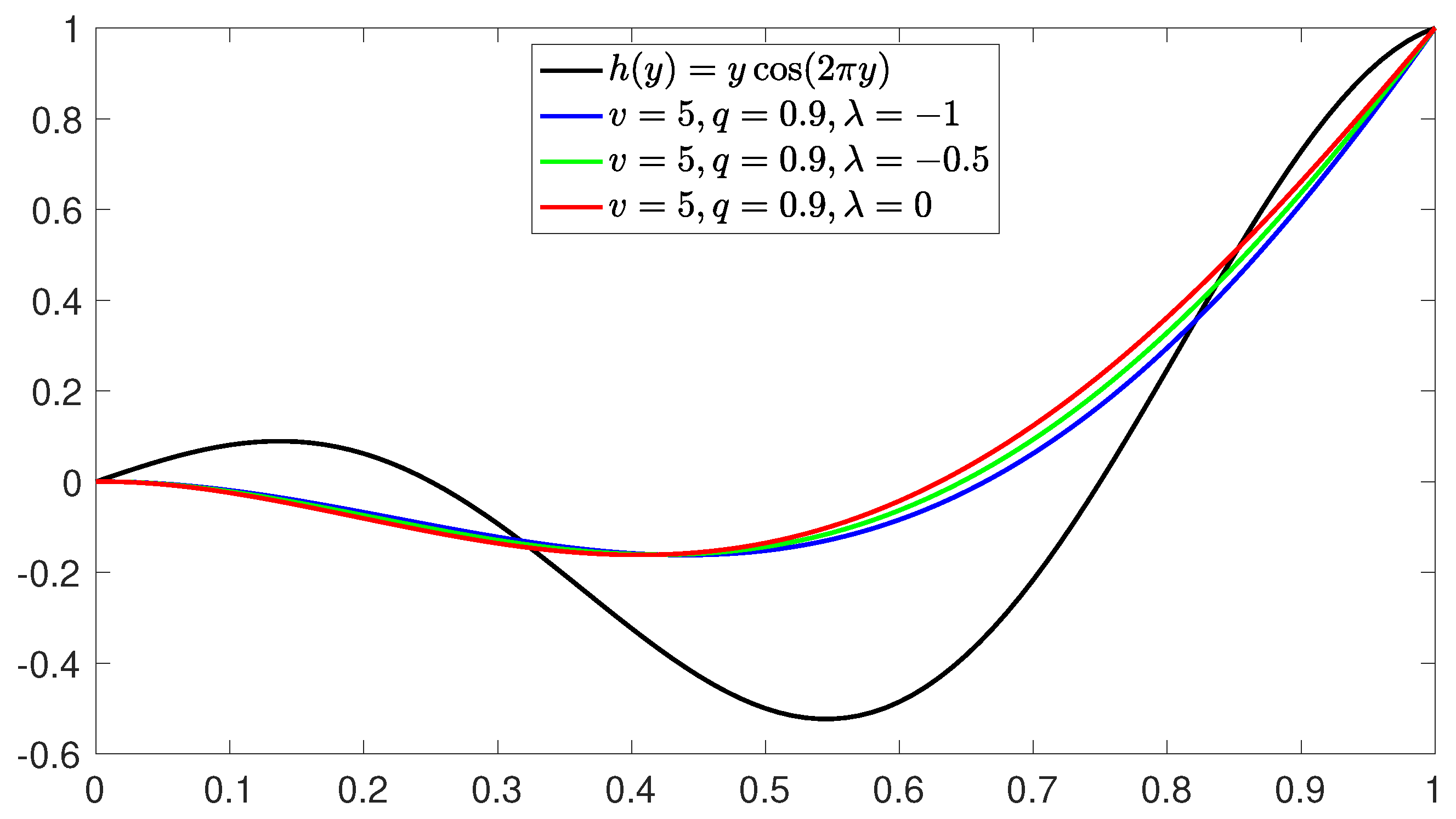
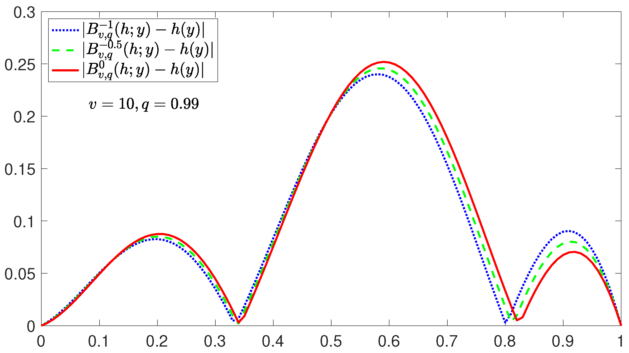
We take the test function $h\left(x\right)=xcos\left(2\pi x\right)$. The graphs of $B_{v,q}^{\lambda }(h;x)$ with $\lambda =1$ are shown in Figure 1. It can be seen from Figure 1 that with the increase in v, $B_{v,q}^1\left(h\right)$ is getting closer and closer to function $h\left(x\right)$. In Figure 2, we fix $v=5$ and $q=0.9$, operators $B_{v,q}^{\lambda }(h;x)$ and $h\left(x\right)$ with different values of the parameters $\lambda$ are shown. It can be seen from Figure 2 that under certain values of $\lambda$ (such as $\lambda =-1$), the convergence behavior of $B_{v,q}^{\lambda }\left(h\right)$ is better than that of $B_{v,q}^0\left(h\right)$, that is q-Bernstein operators. Figure 3 shows the absolute error of $B_{10,0.99}^{-1}(h;x)$, $B_{10,0.99}^{-0.5}(h;x)$ and $B_{10,0.99}^0(h;x)$ on $h\left(x\right)$. Table 1 shows the absolute error bound of $B_{v,q}^{\lambda }(h;x)$ on the function $h\left(x\right)$ when $q=0.9$, $q=0.95$ and so on. As can be seen from Table 1, for fixed q, the closer $\lambda$ is to $-1$, the smaller absolute error bound between $B_{v,q}^{\lambda }\left(h\right)$ and $h\left(x\right)$.

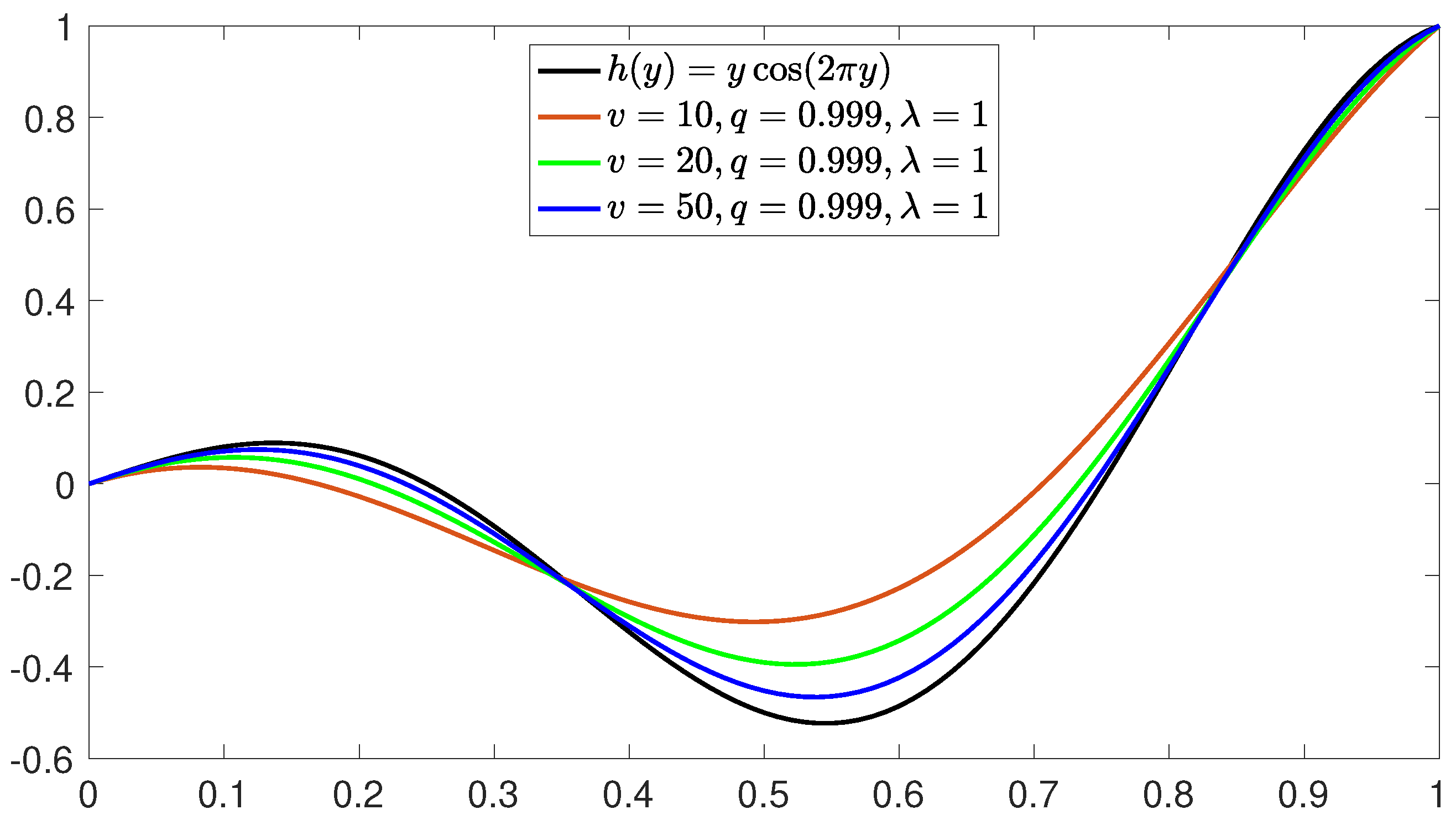
Figure 1. The convergence of $B_{10,0.999}^1(h;x)$, $B_{20,0.999}^1(h;x)$, $B_{50,0.999}^1(h;x)$ to $h\left(x\right)$.

Figure 2. The convergence of $B_{5,0.9}^{-1}(h;x)$, $B_{5,0.9}^{-0.5}(h;x)$, $B_{5,0.9}^0(h;x)$ to $h\left(x\right)$.

Figure 3. Comparison of errors for $B_{10,0.99}^{-1}(h;x)$, $B_{10,0.99}^{-0.5}(h;x)$ and $B_{10,0.99}^0(h;x)$ to $h\left(x\right)$.

Table 1. The absolute error bound of $B_{v,q}^{\lambda }(h;x)$ to $h\left(x\right)$.

q	$\parallel {\mathit{B}}_{\mathit{v},\mathit{q}}^{\mathit{\lambda }}{\left(\mathit{h}\right)-\mathit{h}\parallel }_{\mathbf{\infty }}$
	$\mathit{\lambda }=-\mathbf{1}$	$\mathit{\lambda }=-\mathbf{0.5}$	$\mathit{\lambda }=\mathbf{0}$	$\mathit{\lambda }=\mathbf{0.5}$	$\mathit{\lambda }=\mathbf{1}$
$0.9$	0.242074235	0.242921216	0.243768198	0.244615179	0.245462161
$0.95$	0.146636656	0.147073061	0.147581795	0.14809053	0.148599265
$0.99$	0.074389442	0.074658736	0.07492803	0.075197324	0.075466618
$0.995$	0.066814352	0.067069407	0.067324461	0.067579516	0.06783457
$0.999$	0.06108183	0.061325904	0.061569978	0.061814053	0.062058127
$0.9999$	0.059833655	0.060075309	0.060316963	0.060558617	0.060800271
$0.99999$	0.059709692	0.059951105	0.060192518	0.060433931	0.060675344

References

1. Braha, N.L.; Mansour, T.; Mursaleen, M.; Acar, T. Convergence of λ-Bernstein operators via power series summability method. J. Appl. Math. Comput. 2021, 65, 125–146. [Google Scholar] [CrossRef]
2. Bodur, M.; Manav, N.; Tasdelen, F. Approximation properties of λ-Bernstein-kantorovich-stancu operators. Math. Slovaca 2022, 72, 141–152. [Google Scholar] [CrossRef]
3. Hamal, H.; Sabancigil, P. Kantorovich Type Generalization of Bernstein Type Rational Functions Based on (p, q)-Integers. Symmetry 2022, 14, 1054. [Google Scholar] [CrossRef]
4. Özkan, E.Y.; Aksoy, G. On a New Generalization of Bernstein-type Rational Functions and Its Approximation. Mathematics 2022, 10, 973. [Google Scholar] [CrossRef]
5. Liu, Y.-J.; Cheng, W.-T.; Zhang, W.-H.; Ye, P.-X. Approximation Properties of the Blending-type Bernstein–Durrmeyer Operators. Axioms 2023, 12, 5. [Google Scholar] [CrossRef]
6. Acu, A.M.; Mutlu, G.; Çekim, B.; Yazıcı, S. A new representation and shape-preserving properties of perturbed Bernstein operators. Math. Methods Appl. Sci. 2024, 47, 5–14. [Google Scholar] [CrossRef]
7. Lipi, K.; Deo, N. λ-Bernstein Operators Based on Pólya Distribution. Numer. Funct. Anal. Optim. 2023, 44, 529–544. [Google Scholar] [CrossRef]
8. Aslan, R. Approximation properties of univariate and bivariate new class λ-Bernstein–Kantorovich operators and its associated GBS operators. Comput. Appl. Math. 2023, 42, 34. [Google Scholar] [CrossRef]
9. Yilmaz, Ö.G.; Ostrovska, S.; Turan, M. The continuity in q of the Lupaş q-analogues of the Bernstein operators. J. Math. Anal. Appl. 2024, 529, 126842. [Google Scholar] [CrossRef]
10. Lupaş, A. A q-analogue of the Bernstein operator. In Seminar on Numerical and Statistical Calculus; University of Cluj-Napoca: Cluj-Napoca, Romania, 1987; Volume 9. [Google Scholar]
11. Phillips, G.M. Bernstein polynomials based on the q-integers. Ann. Numer. Math. 1997, 4, 511–518. [Google Scholar]
12. Ostrovska, S. q-Bernstein polynomials and their iterates. J. Approx. Theory 2003, 123, 232–255. [Google Scholar] [CrossRef]
13. Ostrovska, S. On the improvement of analytic properties under the limit q-Bernstein operator. J. Approx. Theory 2006, 138, 37–53. [Google Scholar] [CrossRef]
14. Ostrovska, S. On the Lupaş q-analogue of the Bernstein operator. Rocky Mt. J. Math. 2006, 36, 1615–1629. [Google Scholar] [CrossRef]
15. Dalmanoglu, Ö.; Doğru, O. On statistical approximation properties of Kantorovich type q-Bernstein operators. Math. Comput. Model. 2010, 52, 760–771. [Google Scholar] [CrossRef]
16. Agrawal, P.N.; Finta, Z.; Kumar, A.S. Bernstein-Schurer-Kantorovich operators based on q-integers. Appl. Math. Comput. 2015, 256, 222–231. [Google Scholar] [CrossRef]
17. Mursaleen, M.; Khan, F.; Khan, A. Approximation properties for King’s type modified q-Bernstein-Kantorovich operators. Math. Methods Appl. Sci. 2015, 36, 1178–1197. [Google Scholar] [CrossRef]
18. Cai, Q.-B.; Cheng, W.-T. Convergence of λ-Bernstein operators based on (p, q)-integers. J. Inequalities Appl. 2020, 2020, 35. [Google Scholar] [CrossRef]
19. Khan, A.; Mansoori, M.S.; Khan, K.; Mursaleen, M. Phillips-type q-Bernstein Operators on Triangles. J. Funct. Spaces 2021, 2021, 6637893. [Google Scholar] [CrossRef]
20. Cai, Q.-B.; Aslan, R. Note on a new construction of Kantorovich form q-Bernstein operators related to shape parameter λ. Comput. Model. Eng. Sci. 2022, 130, 1479–1493. [Google Scholar] [CrossRef]
21. Cheng, W.-T.; Nasiruzzaman, M.; Mohiuddine, S.A. Stancu-type Generalized q-Bernstein–Kantorovich Operators Involving Bézier Bases. Mathematics 2022, 10, 2057. [Google Scholar] [CrossRef]
22. Su, L.-T.; Aslan, R.; Zheng, F.-S.; Mursaleen, M. On the Durrmeyer variant of q-Bernstein operators based on the shape parameter λ. J. Inequalities Appl. 2023, 2023, 56. [Google Scholar] [CrossRef]
23. Sabancıgil, P. Genuine q-Stancu-Bernstein–Durrmeyer Operators. Symmetry 2023, 15, 437. [Google Scholar] [CrossRef]
24. Gupta, V. Some approximation properties of q-Durrmeyer operators. Appl. Math. Comput. 2008, 197, 172–178. [Google Scholar] [CrossRef]
25. Gupta, V.; Wang, H. The rate of convergence of q-Durrmeyer operators for 0 < q < 1. Math. Methods Appl. Sci. 2008, 31, 1946–1955. [Google Scholar]
26. Gupta, V.; Finta, Z. On certain q-Durrmeyer type operators. Appl. Math. Comput. 2009, 209, 415–420. [Google Scholar] [CrossRef]
27. Dinlemez, Ü.; Yüksel, İ. Voronovskaja Type Approximation Theorem For q-Szász-Beta-Stancu Type Operators. Gazi Univ. J. Sci. 2016, 29, 115–122. [Google Scholar]
28. Yüksel, İ.; Dinlemez, Ü. Weighted Approximation by the q-Szász-Schurer-Beta Type Operators. Gazi Univ. J. Sci. 2015, 28, 231–238. [Google Scholar]
29. Yüksel, İ.; Dinlemez, Ü.; Altın, B. Approximation by q-Baskakov–Durrmeyer Type Operators of Two Variables. In Computational Analysis: AMAT, Ankara, May 2015 Selected Contributions; Springer International Publishing: Berlin/Heidelberg, Germany, 2016; pp. 195–209. [Google Scholar]
30. Doğru, O.; İçöz, G.; Kanat, K. On the Rates of Convergence of the q-Lupaş-Stancu Operators. Filomat 2016, 30, 1151–1160. [Google Scholar] [CrossRef]
31. Cai, Q.-B.; Zeng, X.M.; Cui, Z. Approximation properties of the modification of Kantorovich type q-Szász operators. J. Comput. Anal. Appl. 2013, 15, 176–187. [Google Scholar]
32. Cai, Q.-B. Approximation properties of the modification of q-Stancu-Beta operators which preserve x2. J. Inequalities Appl. 2014, 2014, 505. [Google Scholar] [CrossRef]
33. Ulusoy, G.; Acar, T. q-Voronovskaya type theorems for q-Baskakov operators. Math. Methods Appl. Sci. 2016, 39, 3391–3401. [Google Scholar] [CrossRef]
34. Khan, K.; Lobiyal, D.K.; Kılıcman, A. Bézier curves and surfaces based on modified Bernstein polynomials. Azerb. J. Math. 2019, 9, 3–21. [Google Scholar]
35. Farin, G. Curves and Surfaces for Computer-Aided Geometric Design: A Practical Guide; Elsevier: Amsterdam, The Netherlands, 2014. [Google Scholar]
36. Sederberg, T.W. Computer Aided Geometric Design 2012. Available online: https://scholarsarchive.byu.edu/facpub/1/ (accessed on 1 September 2021).
37. Farouki, R.T. The Bernstein polynomial basis: A centennial retrospective. Comput. Aided Geometr. Design 2012, 29, 379–419. [Google Scholar] [CrossRef]
38. Gasper, G.; Rahman, M. Basic Hypergeometric Series, Encyclopedia of Mathematics and Its Applications; Cambridge University Press: Cambridge, UK, 1990; Volume 35. [Google Scholar]
39. Kac, V.G.; Cheung, P. Quantum Calculus, Universitext; Springer: New York, NY, USA, 2002. [Google Scholar]
40. Zhou, G.; Chen, S.; Zhao, G. Approximation properties of a new kind of λ-Bernstein operators. 2024; in press. [Google Scholar]
41. Niven, I.; Zuckerman, H.S.; Montgomery, H. An Introduction to the Theory of Numbers, 5th ed.; Wiley: New York, NY, USA, 1991. [Google Scholar]
42. Gadjiev, A.D.; Orhan, C. Some approximation theorem via statistical convergence. Rocky Mt. J. Math. 2002, 32, 129–138. [Google Scholar] [CrossRef]
43. De Vore, R.A.; Lorentz, G.G. Constructive Approximation; Springer: Berlin, Germany, 1993. [Google Scholar]