Abstract
The fashion apparel industry is facing an increasingly growing demand, compounded by the short sales lifecycle and strong seasonality of clothing, posing significant challenges to inventory management in the retail sector. Despite some retailers like Uniqlo and Zara implementing inventory management and dynamic pricing strategies, challenges persist due to the dynamic nature of fashion trends and the stochastic factors affecting inventory. To address these issues, we construct a mathematical model based on the mathematical expression of the deterministic fashion level function, where the geometric Brownian motion, widely applied in finance, is initially utilized in the stochastic fashion level function. Drawing on research findings from deteriorating inventory management and stochastic optimization, we investigate the fluctuation of inventory levels, optimal dynamic pricing, optimal production rates, and profits—four crucial indicators—via Pontryagin’s maximum principle. Analytical solutions are derived, and the numerical simulation is provided to verify and compare the proposed model with deterministic fashion level function models. The model emphasizes the importance of considering stochastic factors in decision-making processes and provides insights to enhance profitability, inventory management, and sustainable consumption in the fashion product industry.
Keywords:
fashion products; dynamic pricing; stochastic optimal control; inventory management; Pontryagin’s maximum principle MSC:
60H05; 60G15; 49N05
1. Introduction
The surge in personalized consumption has led to a continuous increase in consumers’ demand for fashionable clothing. However, fashionable clothing faces challenges such as a short sales lifecycle and strong seasonality. In 2023, both Nike and Adidas encountered excess inventory issues. Nike currently holds inventory worth billion, an increase of compared to the previous year, while Adidas holds inventory worth billion, an increase of . This surplus inventory may result in sluggish sales, excessive capital occupation, and profit decline due to discounted sales, thereby impacting the economic performance and reputation of the brands. Dynamic pricing strategies are closely linked to inventory reduction and increased sales profits. For instance, Uniqlo, GAP, and Zara have embraced dynamic pricing strategies. Among them, Uniqlo’s successful execution of lowering prices at the year’s outset and offering a discount within a quarter has proven more effective in profit enhancement than a price hike at year-end. Although dynamic pricing helps reduce inventory and increase profits, due to the perishability of fashion products, they are greatly influenced by fashion trends, aesthetic trends, and seasonality; thus, the same discount method cannot be applied every time. Therefore, the introduction of a random fashion level function for studying inventory management and dynamic pricing strategies for fashion products is imperative in research.
In recent years, there has been extensive research on dynamic pricing and inventory management issues for fashion products [1,2,3]. Due to their short product lifecycle and high demand volatility, special attention needs to be paid to initial ordering before the sales season starts, as well as replenishment decisions during the sales season [4,5,6]. With the advancement of information technology, dynamic pricing has become easier, thus attracting widespread attention to dynamic pricing strategies in enterprises [7,8,9]. However, unlike general products, fashion apparel belongs to short-lifecycle products, where the value or quantity of most products in inventory will decline over time, similar to characteristics of deteriorating items [10]. Therefore, research on inventory and pricing decisions for fashion products should draw insights from studies on perishable inventory and pricing decisions. Kinkaid and Darling [11] were among the first to investigate the dynamic pricing of perishable items. Gallego and Ryzin [12] developed an inventory model to study dynamic pricing problems with price-sensitive and stochastic demand. Wang et al. [13] and Aladwani et al. [14] studied the optimal dynamic decisions for non-immediately deteriorating items, with the distinction that Aladwani et al. [14] allowed for delayed payments. Rabbani et al. [15] assumed demand to be a time-varying function of price discounts and initial prices, establishing a perishable inventory model dependent on quality, price, and time. Mohammadi et al. [16] developed a multi-objective mixed-integer nonlinear programming model for perishable products with price-dependent demand and deterioration rates. Halim et al. [17] considered the characteristics of nonlinear pricing and linear inventory-dependent market demand for nonlinearly deteriorating items models. Udayakumar [18] analyzed a model for perishable items with price-sensitive demand functions dependent on inventory, allowing for shortages. Almathkour et al. [19] studied a finite horizon inventory model with time-varying demand, non-instantaneously deteriorating items, and backlog. Thus, due to the perishable nature and time-varying characteristics of fashion apparel, implementing joint and time-varying dynamic pricing and production strategies is crucial for managing inventory replenishment and increasing net profits. However, aside from the direct impact of fashion levels, production rates, and demand rates on inventory levels, apparel inventory inevitably faces external stochastic disturbances, such as product returns, stockouts, and human damages [20,21,22,23]. Considering the impact of external stochastic disturbances on inventory levels, research on joint dynamic pricing and inventory strategies in stochastic fashion apparel inventory systems has become a hot topic in recent years.
While previous studies have delved into dynamic pricing and inventory management for deteriorating items, they have disregarded the influence of external random factors. In recent years, there has been extensive research on the impact of stochastic elements on inventory functions, offering valuable insights into inventory management strategies for fashion products [24,25]. The optimal approach to addressing such optimization problems involves utilizing the Pontryagin maximum principle from optimal control theory in conjunction with solving the Hamilton–Jacobi–Bellman (HJB) equation [26]. Alshamriani [27] pioneered the construction and resolution of a stochastic optimal control problem for a production inventory model with deterministic deteriorating items. This involved introducing an Itô stochastic differential equation control system and leveraging the Pontryagin maximum principle to obtain optimal state estimation for linear systems with noise. Li [28] explored joint dynamic pricing and inventory control strategies in a stochastic inventory system with deteriorating items. By applying stochastic optimal control methods, the problem of finding optimal joint dynamic pricing and inventory strategies is transformed into solving the HJB equation. Additionally, Wang et al. [29] investigated joint decision-making in dynamic pricing and production, deriving optimal dynamic pricing and production policies using the Pontryagin maximum principle. Furthermore, Shi et al. [30] proposed a limited-range dynamic pricing and preservation joint strategy for deteriorating items, utilizing the Pontryagin maximum principle to maximize profits. Luo et al. [31] tackled joint dynamic pricing and production policies for stochastic perishable inventory systems, establishing a stochastic dynamic optimization model to maximize total discounted profits. Luo et al. [32] aimed to maximize expected total profits by considering a stochastic optimal control problem for dynamic pricing and inventory management of non-instantaneous perishable items with uncertain demand. In the realm of fashion products, Chen [33] provided a mathematical expression for the fashion level function and characterized the decay pattern of fashionability, investigating a clothing inventory model where demand depends on price and fashion level. Chen [34] explored dynamic pricing strategies and replenishment cycle problems for fashion apparel, taking into account the influence of fashion levels on demand and applying the Pontryagin maximum principle method to derive optimal dynamic pricing strategies and replenishment cycles. However, the fashion level function should not be solely modeled as a monotonically decreasing exponential function; it is also influenced by external factors such as brand image and reputation, seasonal and cyclical variations, and stochastic factors related to consumer demographics and target markets. Therefore, this paper considers the impact of stochastic elements on the fashion level function and introduces a stochastic fashion level function for further investigation.
In considering the influence of random factors on fashion trends, this study draws inspiration from Chen et al. [33] regarding the deterministic fashion level function, proposing a stochastic fashion level function for investigating dynamic pricing and inventory strategies of fashion products. In the fashion level function proposed by Chen et al. [33,34], it exhibits a monotonically decreasing exponential form, aligning with the realistic scenario where the fashion level gradually diminishes over time at a decelerating rate. To retain this fundamental form and introduce the influence of random factors, we refer to the detailed description of geometric Brownian motion in the literature [35,36], noting its widespread application in finance. Additionally, geometric Brownian motion finds application in other fields; for instance, Awudu et al. [37] introduced a stochastic production planning model for a biofuel supply chain under uncertain demand and prices, proposing a stochastic linear programming model within a single-period planning framework to maximize expected profits. Albornoz et al. [38] established a dynamic model for exporters, where firms need to bear sunk costs and fixed costs specific to each foreign market operation, and the profit potential in each foreign market follows geometric Brownian motion. Drawing insights from the varied applications of geometric Brownian motion across different domains, the fashion level function can be viewed as a stochastic process, influenced by multiple factors, including consumer preferences, trend patterns, and market conditions. The path dependency in geometric Brownian motion implies that its drift rate and volatility can vary with the path [39]. Meanwhile, the increments of the path in geometric Brownian motion follow a log-normal distribution. This indicates that changes in the fashion level function follow a log-normal distribution, where its growth rate conforms to a normal distribution [40,41]. This aligns with the typical long-tail distribution observed in the changes of the popularity of fashion products. Hence, this study introduces it for the first time into fashion product research to characterize the variability of the stochastic fashion level function. Geometric Brownian motion provides rich theoretical support for simulating the fashion level function. The combination of its stochastic drift rate and volatility, along with its path-dependent characteristics, allows the simulation results to better reflect changes in the popularity of fashion products, offering a robust theoretical basis for decision-making in the fashion industry. The specific arrangement of this study is as follows: Firstly, we obtain a more realistic stochastic fashion level function; Subsequently, using the Pontryagin maximum principle in stochastic optimal control, we solve the problem of dynamic pricing, inventory control, and profit maximization for fashion products under the joint influence of stochastic inventory and stochastic fashion level function, obtaining the corresponding HJB equation; Next, we derive the Riccati system from the HJB equation and provide an analytical solution using mathematical methods; finally, we validate the proposed new model through numerical simulations, compare it with the model with deterministic fashion level function in terms of inventory, dynamic pricing, and profit, conduct sensitivity analysis on parameters, and draw conclusions of managerial significance. The main contributions of this study are as follows:
- This study integrates the mathematical expression of the deterministic fashion level function, first introducing the widely applied geometric Brownian motion from finance into the fashion level function, making it more realistic;
- It establishes a model for inventory decision-making and dynamic pricing of fashion products under the joint influence of stochastic fashion level function and stochastic inventory level, providing managerial insights for fashion product enterprises;
- It contrasts with the deterministic fashion level function, deducing inventory management strategies and optimal pricing schemes under different fashionability trends, and reveals the significant impact of fashionability trends on profit. By adjusting price system parameters, it discovers that fashion products insensitive to price tend to yield higher profits under the same conditions.
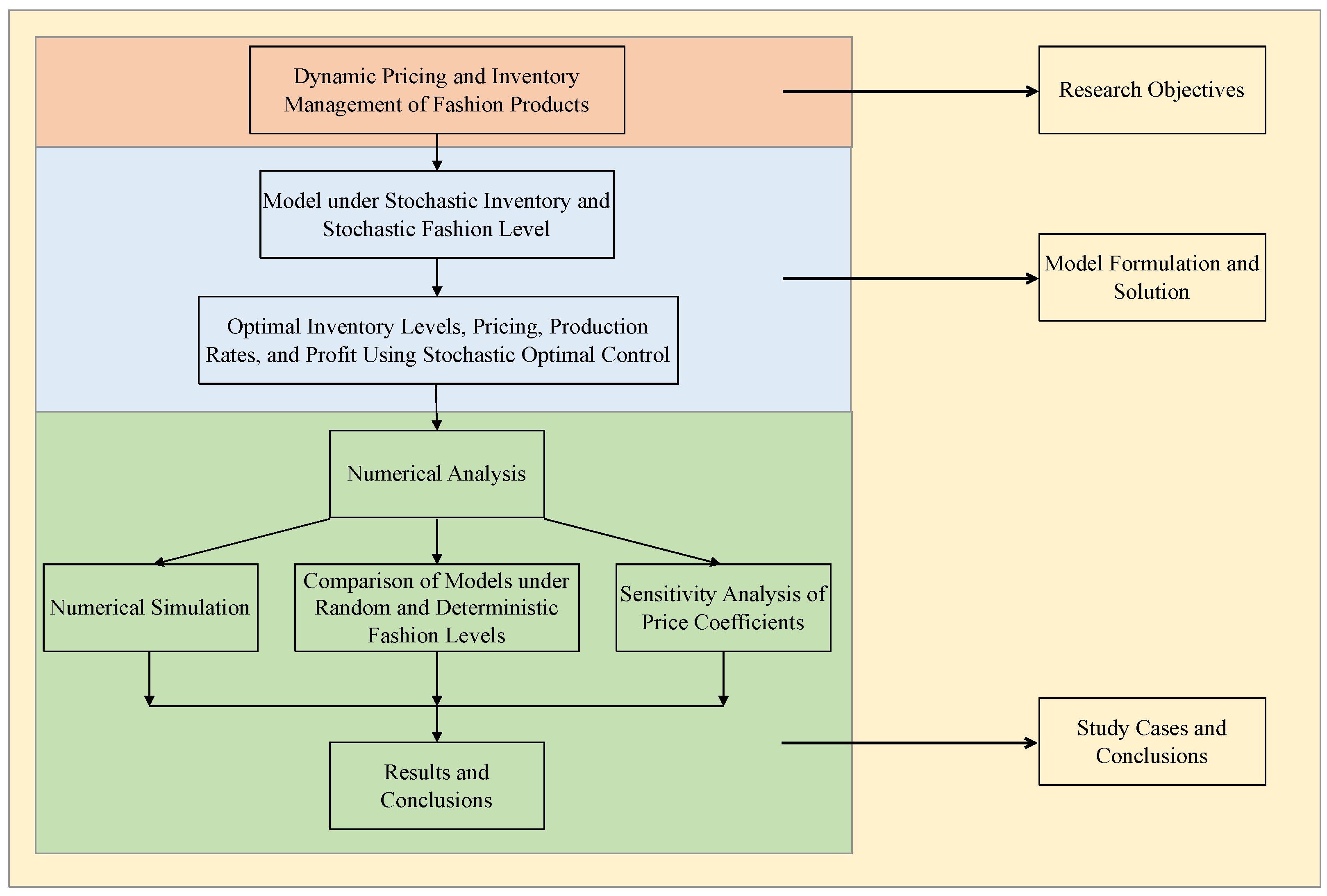
The basic framework of this paper is as follows. In Section 2, we provide some preparation, including the introduction subsequent symbols and stochastic models in this paper. In Section 3, we establish and solve the stochastic dynamic optimization model. In Section 4, we conduct numerical analysis and provide managerial insights. The specific technical roadmap is outlined in Figure 1.

Figure 1.
Technical roadmap.
2. Preliminaries
In this section, we first introduce and define the symbols used in the proposed model. Subsequently, we describe the process of extending a deterministic fashion level function to a stochastic fashion level function. For rigor, we assume that all discussions are conducted within a complete probability space . This probability space encompasses all possible scenarios that we consider, providing a robust mathematical foundation for the development and solution of our model. We first present and explain the necessary symbols, as detailed in Table 1.

Table 1.
List of notations.
This paper focuses on the optimal dynamic pricing and inventory management strategy within a single cycle, without considering multiple cycles or replenishment scenarios. It is assumed that the time parameter is continuous. In paper [34], the authors introduced a fashion level function and provided the following specific expression:
The function is non-negative and monotonically decreasing, with , and is a constant greater than zero. Such a function exhibits the characteristic of exponential decay, as shown in Figure 2b.
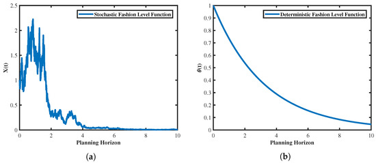
Figure 2.
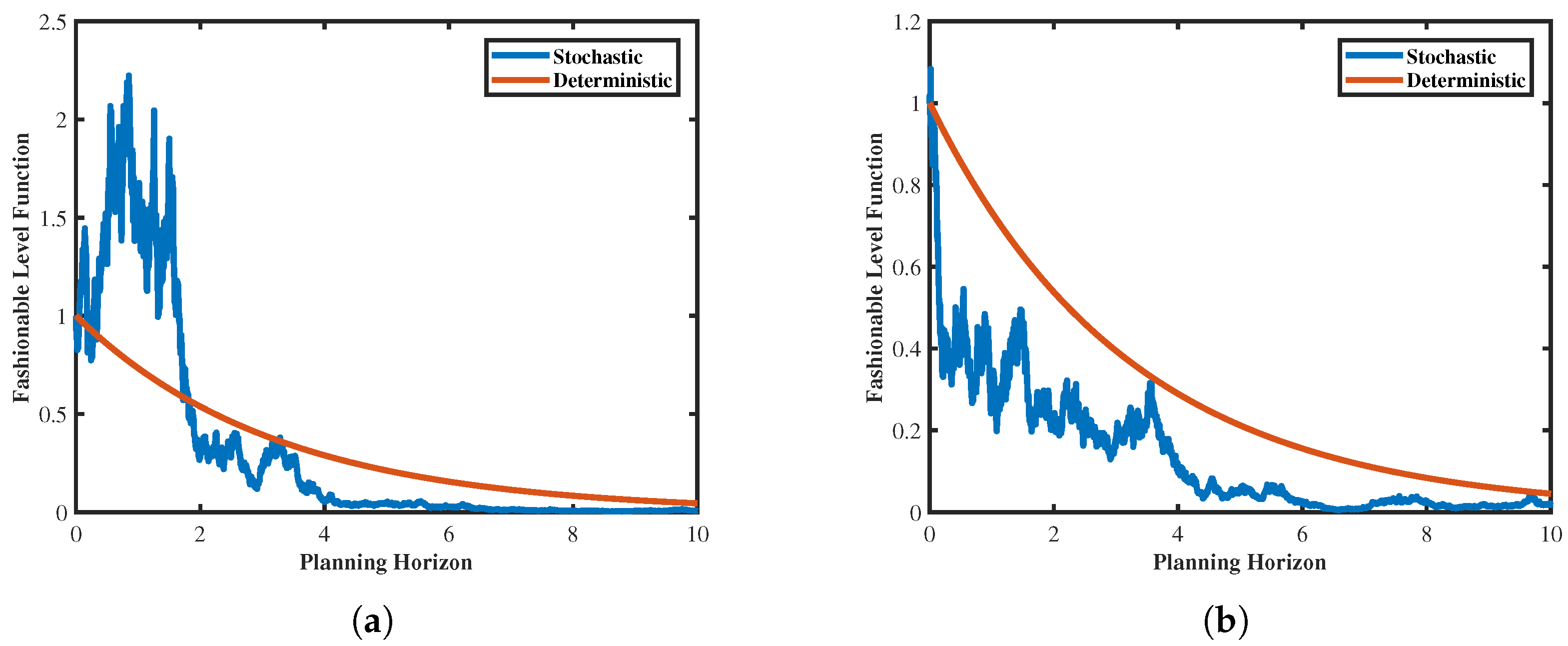
Fashion level function. (a) Stochastic fashion level. (b) Determinstic fashion level.
Through an analysis of fashion product characteristics, it becomes evident that the fashion level function should not only exhibit a declining trend over time but also be influenced by factors such as geography, environment, and statistical characteristics of the product itself. The fashion level function proposed by Chen et al. [33,34] demonstrates a monotonically decreasing exponential form, aligning with the realistic scenario where fashion levels gradually diminish over time at a decelerating rate. In order to maintain this fundamental form and introduce the influence of random factors, we investigate the management characteristics related to fashion products when the fashion level function is perturbed by simple random factors. For simplicity, we employ Brownian motion to model the fashion level function as a stochastic process, where the fashion level function is a stochastic process , with the specific mathematical expression as follows:
Here, , and are two non-zero constants, and is a standard Brownian motion. Through numerical simulations, we can obtain a plot of the fashion level function , as shown in Figure 2a. Comparing these two mathematical expressions and their respective figures, it is evident that Figure 2b exhibits a strictly monotonically decreasing trend, with the rate of decrease slowing down as time passes until the fashion level function gradually approaches zero. In contrast, Figure 2a displays fluctuations but ultimately follows the same trend as Figure 2b. Figure 2a is more in line with the real-world scenario where fashion level function fluctuates over time, reflecting the influence of factors such as regional aesthetic differences and climate uncertainties on fashionability.
For the demand function , as it primarily depends on the price function and the fashion level function , we adopt the following linear function:
where and are two real constants, and, in general, is not equal to zero. It is worth noting that the linear assumption for the demand function is widely used in perishable inventory and management, as seen in the literature [28]. The form we use here is derived from [34].
For the cumulative consumer demand function , we employ the following stochastic integral process (Itô process) to characterize it:
where , is a positive constant, and is a standard Brownian motion, independent of the previously mentioned Brownian motion B.
Finally, for the sake of convenience, we assume that production (replenishment) is instantaneous and infinite, with zero preparation time. According to Alshamrani [27] and Li et al. [28], the continuous dynamic variation of inventory, influenced by production rates and demand rates, satisfies an Itô-type stochastic differential equation:
where . Based on this, by substituting (3) and (4) into (5), we obtain
Equation (6) describes the instantaneous variation in inventory levels. The coefficient in this equation represents the expected change in inventory levels at time t, while the perturbation term from (4) reflects the influence on inventory levels, such as fluctuations due to factors like inventory damage. When inventory levels are positive, consumer demand can be immediately met, and the fashion retailer incurs inventory costs. Therefore, there is a need for a level of inventory to store goods. Conversely, when inventory levels are negative, shortages occur, and customer demands cannot be fulfilled. In such cases, the fashion manufacturer incurs shortage costs. Another interesting question regarding Equation (6) is the statistical behavior of its parameters. In other words, if the system is observable, can we provide estimates for these parameters and study their asymptotic distributions? We will explore such questions in future research.
3. Model Formulation
In this section, based on the background, model assumptions, and dynamic behavior of the system discussed above, we introduce the stochastic control problem under consideration in this paper. We focus solely on fashion products, such as apparel, and define the objective function of their manufacturer:
Here, E represents the mathematical expectation under the probability space mentioned earlier, is the discount factor, represents the production cost at time s when the production rate is , and represents the inventory cost at time s when the inventory level is . For computational convenience, we assume that the functions and are both non-negative and strictly convex, with second-order continuity.
By substituting (3) into (4) and then substituting (4) into (7), and using the martingale property of Itô integrals, we obtain
where K is any left-continuous process; we formulate the manufacturer’s objective function as
Given that the fashion level function satisfies Equation (2) and that the dynamic inventory function is governed by Equation (6), we investigate a stochastic optimal control problem. The objective is to find the optimal production rate and optimal retail price from a permissible control set within a specified time interval to maximize the company’s total profit during this time span.
Based on the previous analysis, we already understand that the optimal production rate and optimal retail price are both stochastic processes that depend on inventory level function I and fashion level function X. Therefore, we can define the permissible control set as follows:
where and are two stochastic processes that depend on inventory I and fashion level function X, representing the production rate and retail price, respectively. The values of I and X are determined by (2) and (6), respectively. We denote the optimal production rate and optimal retail price as
Consequently, we can formulate the model as the following optimization problem:
where and satisfy Equations (2) and (6), respectively. For the sake of brevity, in the following discussions, we omit the dependence on t in the stochastic processes or functions such as , , and . To find the optimal control strategy, we employ dynamic programming, assuming that represents the profit function.
Proposition 1.
Under the assumptions of the model outlined above, the Hamilton–Jacobi–Bellman (HJB) equation corresponding to Problem (9) is as follows:
with boundary condition
Proof.
The proof idea of this proposition involves using Itô’s lemma and knowledge of stochastic control. Specifically, it can be divided into the following three steps:
- Step 1: Using stochastic control theory, we define the necessary functions and for the proof, explain their meanings, and provide the relationship between and .
Given an initial value with , by employing the optimal strategy between and T, we have
where , . To simplify the proof, rewrite in the following form:
For convenience in our discussion, we denote and as and , respectively. We also define
where and are understood as control functions within the interval . Then, the expected value function can be expressed as
- Step 2: Using Itô’s formula, we compute and , explaining their meanings and illustrating their relationship.
For any sufficiently small , according to the dynamic programming principle, the value function can be written as
Now, assuming that achieves its optimum at , we have
Due to the optimality of the value function, also satisfies the following equation:
We also rearrange as follows:
Noting the adaptivity of the processes and and utilizing Itô’s formula, we obtain the following expression:
- Step 3: We simplify the above result to obtain an equation.
Taking the expected value on both sides of the above equation and substituting Equations (2) and (6), we obtain
Next, substituting Equation (21) into Equation (16), we can obtain
After simplification, we obtain the equation
Dividing both sides of the equation by and substituting the form of Equation (9) into Equation (23), we have
Here, we have established this proposition. □
Now, for a function V, let us denote and .
Proposition 2.
Let . If there are no constraints on the control variables and , then, under the joint influence of stochastic inventory and stochastic fashion level function, the optimal dynamic pricing and the optimal production rate for the fashion supply system have the following behavior:
where .
Proof.
By taking the first derivatives of the HJB equation (Equation (3)) with respect to the production rate and retail price, we can obtain the optimal production rate and the optimal dynamic pricing , as given in (25). □
To facilitate illustration and align with most production control models, we adopt the assumption that production cost and inventory cost are both quadratic, as expressed in the following form (and as referenced in [42]):
where and . In this case, the HJB equation from Proposition 1 will take the following form:
In this way, we can also derive that the optimal production rate and optimal dynamic pricing from Proposition 2 have the following forms:
At the end of this section, based on the form of the HJB equation, we consider a utility function with a quadratic form as follows:
Proposition 3.
Assuming that the utility function is given as shown in (29), the Riccati system for this model is as follows:
where .
Proof.
For the Riccati system in Proposition 3, elementary calculations can show that
where . With the expression for , we can further obtain the expressions for and as follows:
and
Similarly, from , , and , we can also provide the expressions for , , and as follows:
where
The constants , , , , and can all be determined from the terminal condition in (11). This allows us to solve for the optimal production rate as follows:
and the optimal pricing as
4. Results and Discussions
4.1. Numerical Analysis
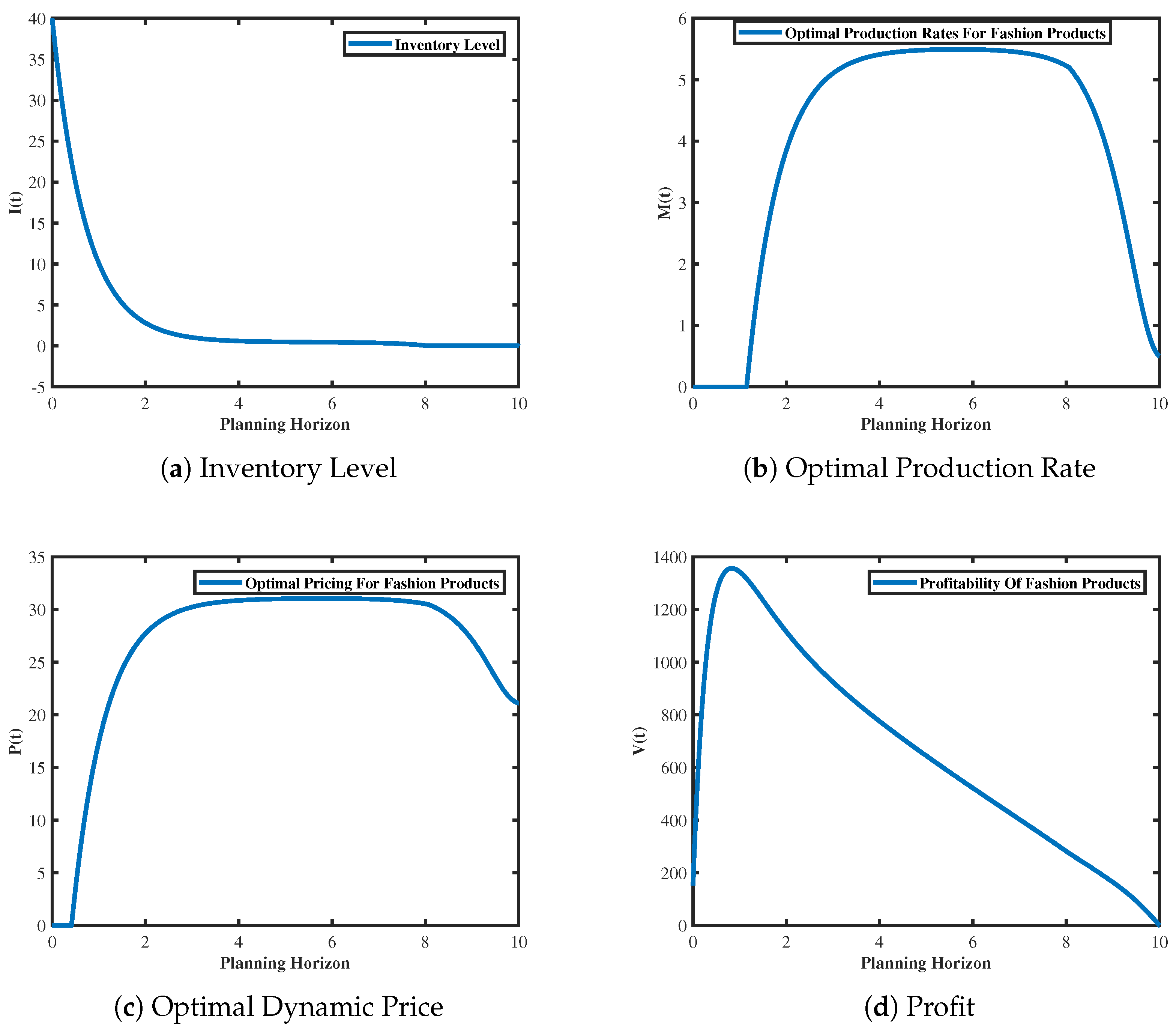
To validate the effectiveness of the mathematical model presented in Section 3, we drew upon the parameters obtained from numerical simulations in the studies in [34,42]. The parameters of our model are specified as follows: initial demand quantity 40, the demand per unit of time , the price coefficient , time range to , initial fashion level , fashion decay factor , inventory drift parameter , and volatility parameter of the fashion level function . Using Matlab 2017b code, we obtained graphical representations of the inventory function (see Figure 3a), the optimal production rate (see Figure 3b), the optimal dynamic pricing (see Figure 3c), and the profit (see Figure 3d). These figures better illustrate the underlying mechanisms in the model.
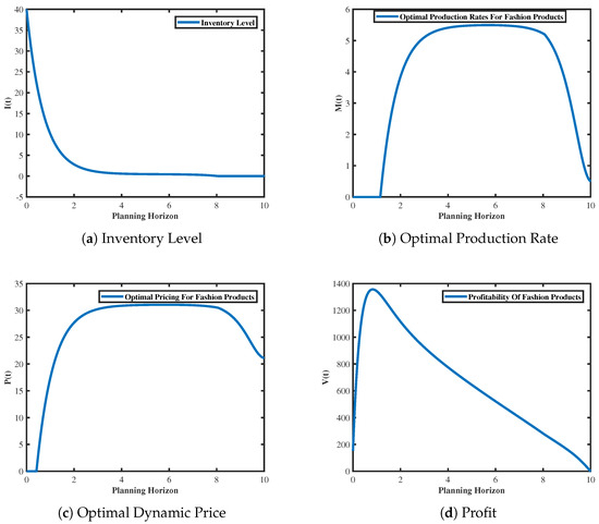
Figure 3.
Inventory level, dynamic pricing, optimal production rate, and profit sample track trends under stochastic fashion level.
Figure 3a shows the inventory dynamics of fashion products within the planning horizon under the influence of stochastic fashionability. As shown, under the optimal joint dynamic pricing and production control strategy, the optimal inventory level of fashion products decreases over time, eventually stabilizing at zero. At , the inventory function rapidly declines from 40 to 4; subsequently, the decrease becomes gradual, ultimately approaching zero. This is because, at the beginning of the sales period, the inventory function declines rapidly due to the high fashion level of the product and the relatively low factory production rate. This trend aligns with the real−life variation in fashion product inventories, indicating a balance between production and sales at the end of the fashion product sales period, with minimal product surplus.
Figure 3b presents the optimal production rate of fashion products within the planning horizon under the influence of stochastic fashion level function. As depicted, the production rate of fashion products exhibits an initial sharp increase, followed by a period of stability before decline. During the time interval from 0 to 1, the optimal production rate is 0, indicating that initial fashion product inventory obviates the need for production. Subsequently, as inventory levels decrease significantly, the production rate of products notably rises, peaking at 5.201 at and sustaining until . Thereafter, the production rate of fashion products begins to decline, reaching at . This demonstrates that, at the end of the sales cycle, the optimal production rate of fashion products gradually approaches the ideal state of 0, ultimately eliminating surplus inventory production.
In Figure 3c, the optimal pricing of fashion products within the planning horizon under the influence of stochastic fashion level function is depicted. It can be observed that optimal pricing exhibits a trend of initially sharp increase, followed by a period of stability before declining. For instance, at , the optimal dynamic pricing reaches a peak of , which persists until , before rapidly decreasing. This phenomenon can be attributed to the initial high fashion level function and good sales performance of the fashion products, leading to a rapid increase to the peak. However, as time progresses, market saturation occurs, accompanied by a decline in product fashionability, prompting the adoption of discount sales strategies. This implies that the optimal pricing strategy allows product pricing to reach a relatively ideal level in the short term and rapidly decrease towards the end of the sales cycle, facilitating inventory clearance. Within the planning horizon and under the influence of stochastic fashion level function, Figure 3d depicts the profitability of fashion products. As shown from this figure, the profit function also exhibits a trend of initially rising and then declining. A notable observation from the figure is that the profit reaches its peak of 1368 at , with a significant upward trend observed during the time interval from 0 to 1. This trend is closely related to the substantial decrease in the inventory function and the significant increase in the optimal pricing of fashion products during the initial period, enabling the enterprise to maximize profits in the short term and avoid losses throughout the sales period.
4.2. Comparison between Stochastic Fashion Level and Deterministic Fashion Level
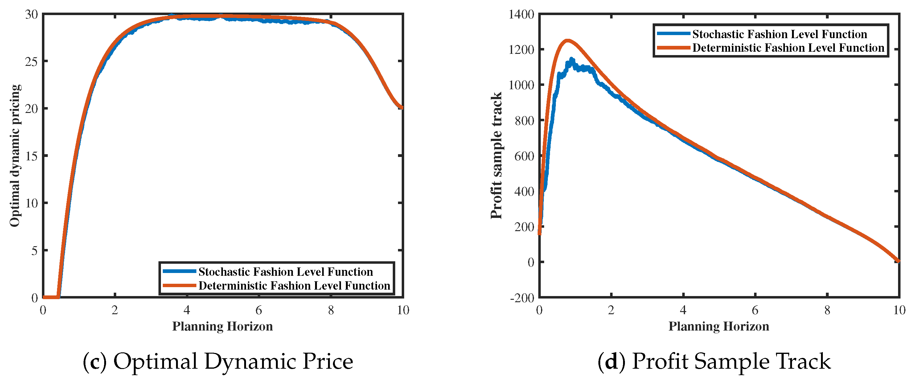
To elucidate the feasibility and practicality of the model, we compared it with the results of deterministic fashion level [34], investigating the variations in inventory function, optimal production rate, dynamic pricing, and profit—four key performance indicators. Interestingly, Figure 4 shows that the stochastic fashion level function indeed exerts a noticeable influence on the aforementioned metrics of fashion products discussed earlier. By comparing the stochastic fashion level model with the deterministic one, we derived some meaningful managerial insights.
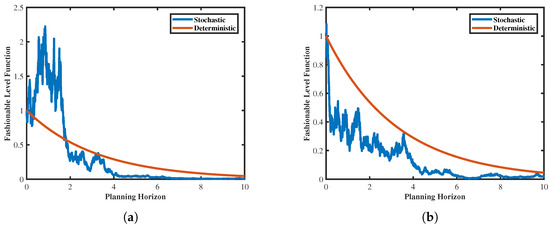
Figure 4.
The relationship between stochastic and deterministic fashion levels. (a) Stochastic fashion level declines slower than deterministic fashion level. (b) Stochastic fashion level declines faster than deterministic fashion level.
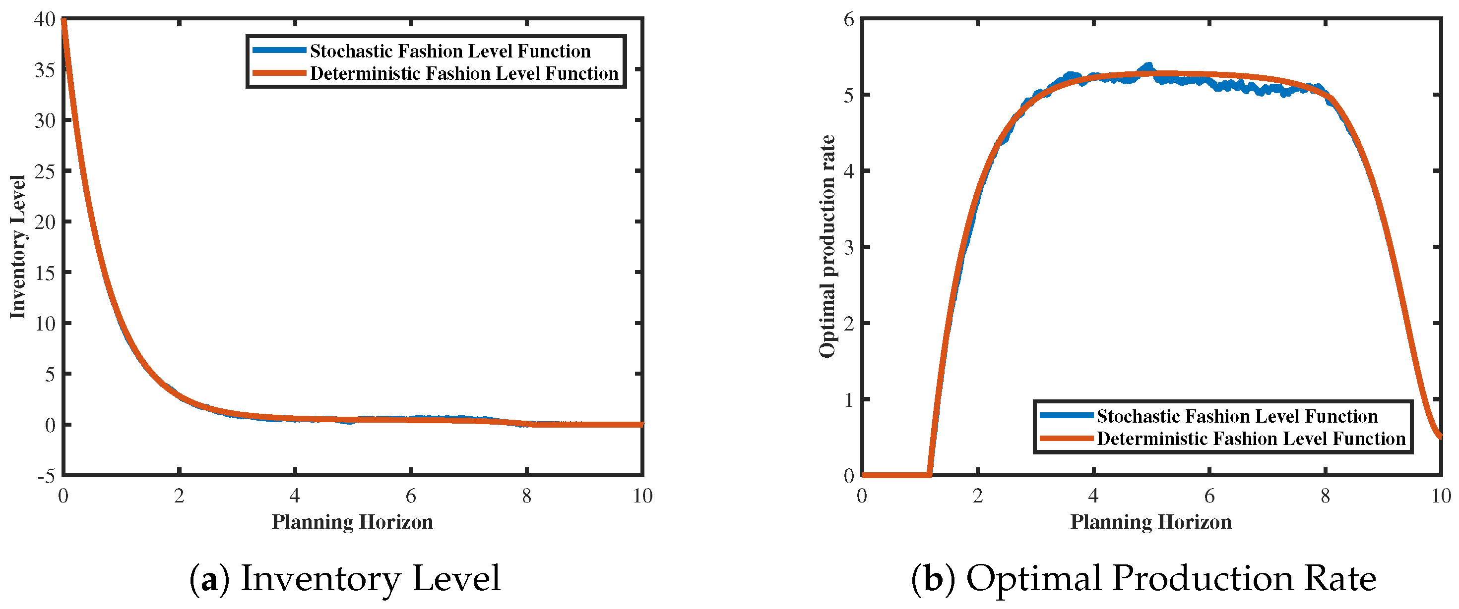
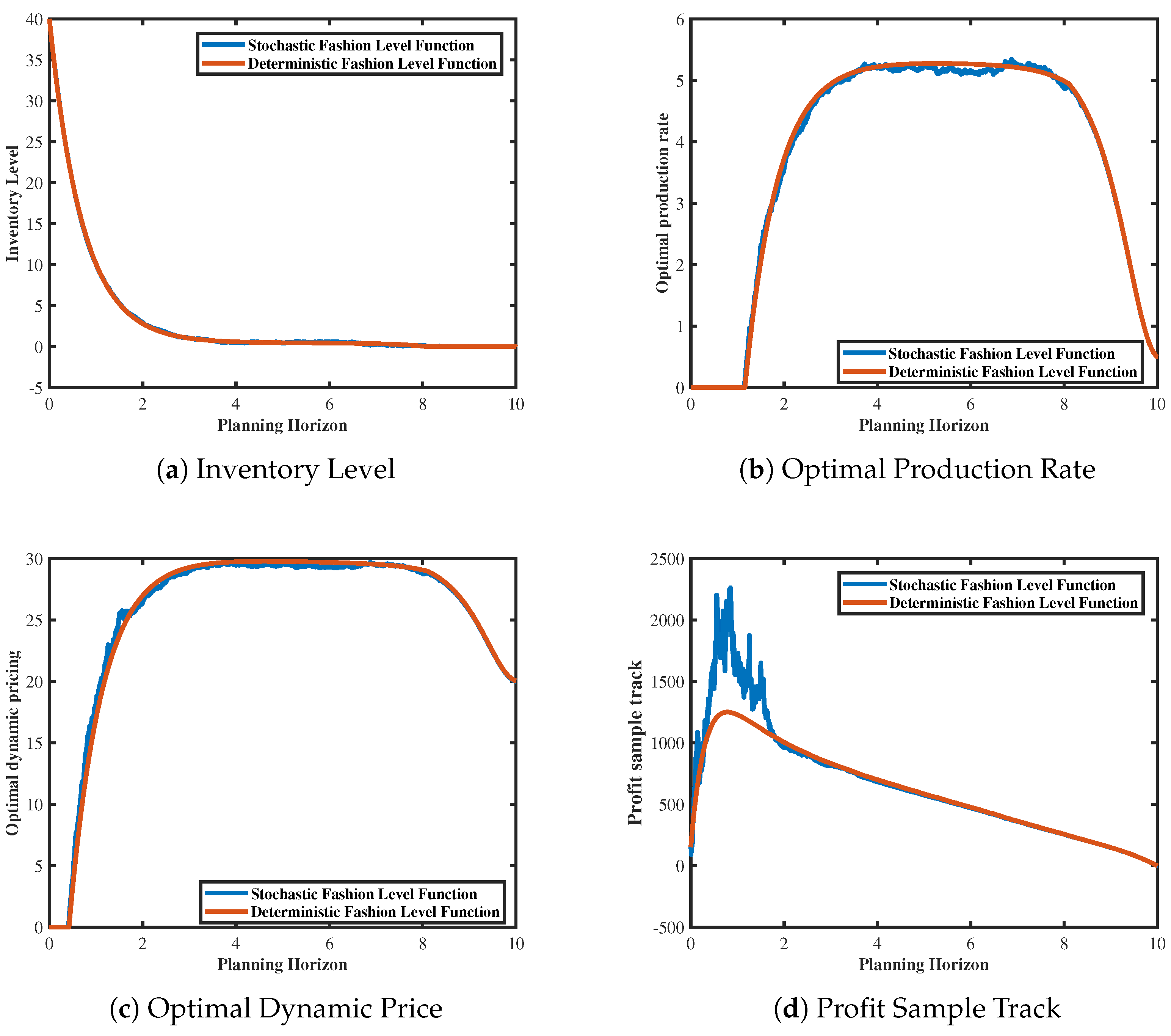
Based on Figure 5, the trends in inventory function, optimal production rate, optimal dynamic pricing, and profit of fashion products are shown within the planning horizon when the stochastic fashion level function decreases faster than the deterministic fashion level function. Although the inventory function, optimal production rate, optimal dynamic pricing, and profit exhibit similar trends under both models, there is a notable difference in profit, with profits being smaller under the stochastic fashion level function model compared to the deterministic fashion level function model. Specifically, the inventory function still demonstrates a rapid decline, while the optimal production rate and optimal dynamic pricing show a similar trend of initially rapid increase, followed by a period of stability, and then rapid decrease. In contrast, the optimal production rate and optimal dynamic pricing under the deterministic fashion level model are slightly better than those under the stochastic fashion level model. The difference in profit is significant compared to the other three factors, with the profit peak under the deterministic fashion model being 1250, while, under the stochastic fashion model, it is only 1150. This is because, when the fashion of fashion products decreases rapidly, consumer attractiveness diminishes, which may be influenced by market saturation, fashion cycles, and other factors, causing the fashion product to become less preferred by consumers. Therefore, companies may consider conducting in−depth market research to understand consumer needs and preferences, timely adjust product positioning to meet market demand, enhance brand image through effective branding and PR activities to increase brand visibility and reputation, continually monitor consumer feedback and market dynamics, and timely adjust corporate strategies and product policies to maintain sensitivity and adaptability to market changes, thus preemptively avoiding rapid declines in fashionability. However, contrary to expectations, Figure 6 demonstrates that, when the deterministic fashion function decreases faster than the stochastic fashion level function, the trends in inventory function, optimal production rate, optimal dynamic pricing, and profit of fashion products are opposite to those shown in the figure. Specifically, under both models, although the inventory function, optimal production rate, and optimal dynamic pricing exhibit similar trends across different price coefficients, contrary to the depicted scenario, the stochastic fashion model slightly outperforms the deterministic fashion model in terms of the optimal production rate and optimal dynamic pricing. However, there is a significant difference in profit peaks. For instance, under the stochastic fashion model, the profit peak is 2210, whereas, under the deterministic fashion model, it is only 1250. This may be attributed to excellent product design and quality, as well as associations with influential individuals or celebrities, which enhance product attractiveness and fashion, along with factors such as increasing the visibility and influence of fashion products on social media platforms and digital channels. Therefore, companies should invest resources and efforts in developing innovative and unique products, enhancing brand visibility and influence through effective brand positioning, promotion, and marketing activities, establishing a fashion−related brand image, leveraging digital technology and social media platforms to expand brand exposure, and collaborating with influential individuals, celebrities, or other brands to enhance product fashion and attractiveness.
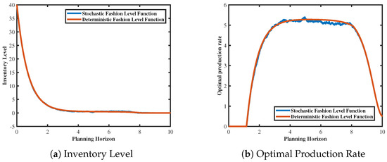
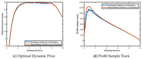
Figure 5.
Inventory level, dynamic pricing, optimal production rate, and profit sample track trends under faster decline of stochastic fashion level.
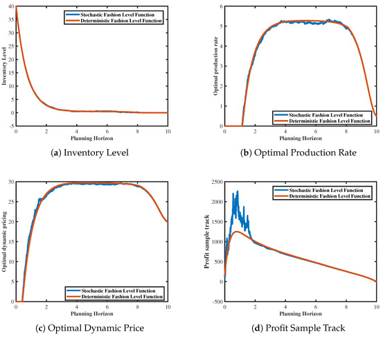
Figure 6.
Inventory level, dynamic pricing, optimal production rate, and profit sample track trends under stochastic fashion level declines slower than deterministic fashion level.
4.3. Sensitivity Analysis of Price Coefficients
To examine the impact of price coefficients on the model outcomes, we considered a range of different coefficient values and studied the variations in the inventory function, optimal production rate, optimal dynamic pricing, and profit—four crucial performance indicators in the model. These analyses demonstrate that price coefficients are indeed significant factors that influence fashion product profits. Moreover, by varying the initial inventory levels and comparing the key performance indicators in the model under different price coefficient values, we obtained more generalizable conclusions.
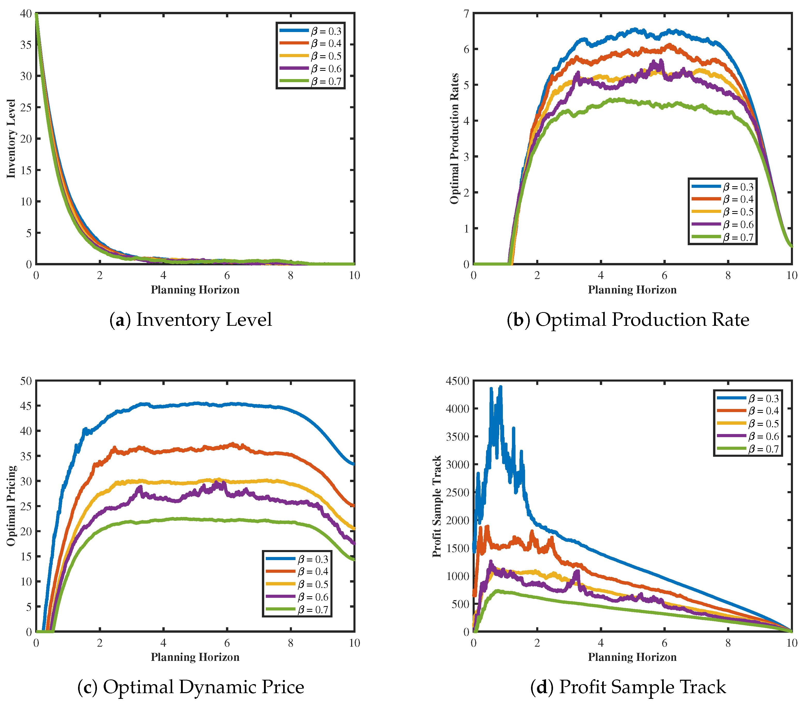
Based on the illustration in Figure 7, the impact of different price coefficients on the inventory function, optimal production rate, optimal dynamic pricing, and profit of fashion products within the planning horizon is demonstrated. It is observed that the trends in the inventory function, optimal production rate, optimal dynamic pricing, and profit remain largely similar across different price coefficients, with lower coefficients yielding higher profits. Specifically, the inventory levels of fashion products exhibit minor differences across various price coefficients, indicating the robustness of the optimal joint dynamic pricing and production strategy concerning the inventory levels of fashion products under different coefficient values. Furthermore, similar trends are observed for the optimal production rate and pricing, with lower price coefficients corresponding to higher peak values in both aspects across five different coefficient scenarios. Regarding the profit, an examination of the sample trajectory plots under various price coefficients in Figure 7d reveals a common trend of initial increase followed by a decrease across different coefficient conditions, with lower price coefficients leading to higher profits. This is because low-price-sensitivity fashion products refer to those for which consumers are less responsive to price changes, instead prioritizing factors such as product quality, design, and brand image, among others, over price considerations. As a result, consumers tend to purchase them based on these attributes rather than being swayed by price fluctuations. A notable observation derived from the findings is that, under equivalent circumstances, fashion products with lower price sensitivity tend to achieve greater profits.
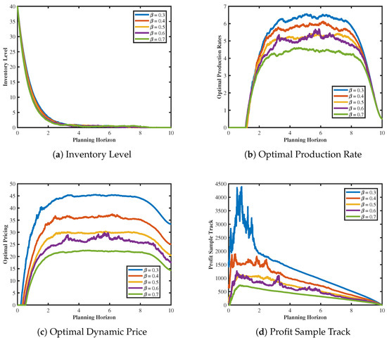
Figure 7.
Inventory level, dynamic pricing, optimal production rate, and profit sample track trends under different coefficient values.
Figure 8 illustrates the variation trend in profit under the influence of different initial inventory levels within the planning horizon. As depicted, despite the varying initial inventory levels, profit trajectories all exhibit a common trend of initial ascent followed by descent. However, it is observed that lower price coefficients correspond to higher profit peaks. Specifically, at an initial inventory of 800 at , profit reaches its maximum value of 1640 when the price coefficient is , whereas, with a coefficient of , the profit peak is only 550. From this, we can derive a more universally applicable conclusion: under equivalent conditions, fashion products with low price sensitivity are more likely to yield greater profits. Therefore, it is advisable for businesses to moderately introduce products with high price sensitivity and to engage in flexible production planning.
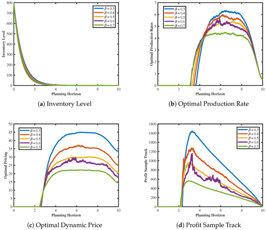
Figure 8.
Inventory level, dynamic pricing, optimal production rate, and profit sample track trends under different coefficient values.
5. Model Drawbacks and Future Improvements
This model explores the combined influence of stochastic fashion level function and stochastic inventory levels on inventory decisions and dynamic pricing of fashion products, extending upon the deterministic fashion level function proposed by Chen et al. [33,34]. Through analysis of the deterministic fashion level function, we identified its exponential form that monotonically decreases over time. To maintain this basic form and introduce stochastic elements, references [35,36] proposed a stochastic fashion level function resembling geometric Brownian motion, providing theoretical insights and management guidance.
However, further research has uncovered two limitations and potential improvements:
Firstly, in the equations governing stochastic inventory and fashion level functions, we initially assumed they are independently driven by Brownian motions and in Equations (2) and (6), respectively. Subsequent studies have indicated mutual influences between stochastic inventory level and fashion level, suggesting that their driving processes should not be independent. Therefore, future research plans to use two correlated Brownian motions to separately drive stochastic inventory and fashion level functions, aiming for a more realistic model;
Secondly, the current study focuses on optimal dynamic pricing and inventory management strategies within a single cycle, without considering multiple cycles or replenishment. To refine the model, we propose replacing Brownian motion with Poisson processes to redefine the equation for the stochastic inventory function. Poisson processes are suitable for modeling stochastic processes with jumps, thereby better capturing scenarios involving specific replenishment times. This will be a key focus of future research.
These enhancements will enhance the realism and comprehensiveness of our model, facilitating a more accurate understanding and optimization of management decisions for fashion products.
6. Conclusions
In summary, this study investigates the impact of stochastic factors on both the inventory function and the fashion level function of fashion products. A stochastic inventory model is developed, and four key performance indicators—inventory level, optimal production rate, optimal dynamic pricing, and profit—are studied under this scenario. The findings and managerial implications are as follows:
Firstly, the optimal dynamic pricing and production rate of fashion products exhibit a linear feedback relationship with the inventory level and fashion level function. This enables firms to accurately devise effective strategies for dynamic pricing and production rate as inventory levels evolve over time, ensuring relatively stable decision-making;
Secondly, comparing deterministic fashion level function models with stochastic ones reveals significant effects of fashion level changes on the four key performance indicators. This underscores the importance for firms to invest in innovative designs and unique product features, enhance brand recognition and influence, expand brand exposure through digital technology and social media platforms, and collaborate with influential individuals or brands to boost product appeal and fashionability;
Thirdly, concerning the price coefficient in the inventory function, our model suggests that products with lower price sensitivity tend to yield higher profits under similar conditions. Thus, firms should adjust their production planning accordingly by introducing products with higher price sensitivity while remaining flexible. However, it is acknowledged that current inventory models are somewhat theoretical, and future research will explore statistical regularities in model parameters.
Author Contributions
Conceptualization, W.L. and L.Y.; methodology, W.L. and L.Y.; software, W.L.; validation, W.L. and L.Y.; formal analysis, L.Y.; writing—original draft preparation, W.L.; writing—review and editing, W.L. and L.Y.; visualization, W.L.; supervision, L.Y. All authors have read and agreed to the published version of the manuscript.
Funding
This work was supported by the National Natural Science Foundation of China (Grant No. 11971101).
Institutional Review Board Statement
Not applicable.
Informed Consent Statement
Not applicable.
Data Availability Statement
The data presented in this study are available upon request from the corresponding author.
Acknowledgments
The authors thank the editor and the referees for their valuable comments and suggestions, which greatly improved the quality of this paper.
Conflicts of Interest
The authors declare no conflicts of interest.
References
- Wu, K.S.; Ouyang, L.Y.; Yang, C.T. An optimal replenishment policy for non-instantaneous deteriorating items with stock-dependent demand and partial backlogging. Int. J. Prod. Econ. 2006, 101, 369–384. [Google Scholar] [CrossRef]
- Maihami, R.; Kamalabadi, I.N. Joint pricing and inventory control for non-instantaneous deteriorating items with partial backlogging and time and price dependent demand. Int. J. Prod. Econ. 2012, 136, 116–122. [Google Scholar] [CrossRef]
- Modak, I.; Bardhan, S.; Giri, B.C. Dynamic pricing and replenishment policy under price, time, and service level-dependent demand and preservation investment. J. Manag. Anal. 2024, 1–26. [Google Scholar] [CrossRef]
- Ouyang, L.Y.; Wu, K.S.; Yang, C.T. A study on an inventory model for non-instantaneous deteriorating items with permissible delay in payments. Comput. Ind. Eng. 2006, 51, 637–651. [Google Scholar] [CrossRef]
- Tsao, Y.C.; Sheen, G.J. Dynamic pricing, promotion and replenishment policies for a deteriorating item under permissible delay in payments. Comput. Oper. Res. 2008, 35, 3562–3580. [Google Scholar] [CrossRef]
- Liu, S.; Wang, J.; Wang, R.; Zhang, Y.; Song, Y.; Xing, L. Data-driven dynamic pricing and inventory management of an omni-channel retailer in an uncertain demand environment. Expert Syst. Appl. 2024, 244, 122948. [Google Scholar] [CrossRef]
- Maihami, R.; Abadi, I.N.K. Joint control of inventory and its pricing for non-instantaneously deteriorating items under permissible delay in payments and partial backlogging. Math. Comput. Model. 2012, 55, 1722–1733. [Google Scholar] [CrossRef]
- Jodrá, P.; Jiménez-Gamero, M. A note on the Log-Lindley distribution. Insur. Math. Econ. 2016, 71, 189–194. [Google Scholar] [CrossRef]
- Couzon, P.; Ouazene, Y.; Yalaoui, F. Joint optimization of dynamic pricing and lot-sizing decisions with nonlinear demands: Theoretical and computational analysis. Comput. Oper. Res. 2020, 115, 104862. [Google Scholar] [CrossRef]
- Setiawan, R. Game theory approach to determine economic order quantity of probabilistic two-level supply chain for deteriorating item with time dependent holding cost. AIP Conf. Proc. 2019, 2194, 020114. [Google Scholar]
- Kinkaid, W.; Darling, D.A. An inventory pricing problem. J. Math. Anal. Appl. 1963, 7, 183–208. [Google Scholar] [CrossRef]
- Gallego, G.; Hu, M. Dynamic pricing of perishable assets under competition. Manag. Sci. 2014, 60, 1241–1259. [Google Scholar] [CrossRef]
- Wang, Y.; Zhang, J.; Tang, W. Dynamic pricing for non-instantaneous deteriorating items. J. Intell. Manuf. 2015, 26, 629–640. [Google Scholar] [CrossRef]
- Aladwani, R.M.; Benkherouf, L.; Almathkour, F. Optimal inventory policies for finite horizon deterministic inventory models for non-instantaneous deteriorating items and permissible-delay in payment. Int. J. Syst. Sci. Oper. Logist. 2023, 10, 2235268. [Google Scholar] [CrossRef]
- Rabbani, M.; Zia, N.P.; Rafiei, H. Joint optimal dynamic pricing and replenishment policies for items with simultaneous quality and physical quantity deterioration. Appl. Math. Comput. 2016, 287, 149–160. [Google Scholar] [CrossRef]
- Mohammadi, Z.; Barzinpour, F.; Teimoury, E. A location-inventory model for the sustainable supply chain of perishable products based on pricing and replenishment decisions: A case study. PLoS ONE 2023, 18, e0288915. [Google Scholar] [CrossRef] [PubMed]
- Halim, M.A.; Paul, A.; Mahmoud, M.; Alshahrani, B.; Alazzawi, A.Y.; Ismail, G.M. An overtime production inventory model for deteriorating items with nonlinear price and stock dependent demand. Alex. Eng. J. 2021, 60, 2779–2786. [Google Scholar] [CrossRef]
- Udayakumar, R. An EOQ model for non-instantaneous deteriorating items with time-dependent demand under partial backlogging. J. Manag. Anal. 2022, 9, 514–531. [Google Scholar] [CrossRef]
- Almathkour, F.; Benkherouf, L. Optimal policies for finite horizon model with time-varying demand rate, non-instantaneous deterioration and backlogging. Int. J. Syst. Sci. Oper. Logist. 2023, 10, 2041128. [Google Scholar] [CrossRef]
- Xie, B.; Gao, Y. On the long-run average cost minimization problem of the stochastic production-inventory models. J. Ind. Manag. Optim. 2024, 20, 1823–1844. [Google Scholar] [CrossRef]
- Benkherouf, L. On a stochastic inventory model with a generalized holding costs. Eur. J. Oper. Res. 2007, 182, 730–737. [Google Scholar] [CrossRef]
- Onggo, B.S.; Panadero, J.; Corlu, C.G.; Juan, A.A. Agri-food supply chains with stochastic demands: A multi-period inventory routing problem with perishable products. Simul. Model. Pract. Theory 2019, 97, 101970. [Google Scholar] [CrossRef]
- Muriana, C. An EOQ model for perishable products with fixed shelf life under stochastic demand conditions. Eur. J. Oper. Res. 2016, 255, 388–396. [Google Scholar] [CrossRef]
- Ouaret, S. Production control problem with semi-Markov jump under stochastic demands and deteriorating inventories. Appl. Math. Model. 2022, 107, 85–102. [Google Scholar] [CrossRef]
- Pan, X.; Li, S. Optimal control of a stochastic production–inventory system under deteriorating items and environmental constraints. Int. J. Prod. Res. 2015, 53, 607–628. [Google Scholar] [CrossRef]
- Das, S.; Mandal, G.; Akhtar, F.; Shaikh, A.A.; Bhunia, A.K. Pricing and dynamic service policy for an imperfect production system: Extended Pontryagin’s maximum principle for interval control problems. Expert Syst. Appl. 2024, 238, 122090. [Google Scholar] [CrossRef]
- Alshamrani, A.M. Optimal control of a stochastic production-inventory model with deteriorating items. J. King Saud Univ.-Sci. 2013, 25, 7–13. [Google Scholar] [CrossRef]
- Li, S.; Zhang, J.; Tang, W. Joint dynamic pricing and inventory control policy for a stochastic inventory system with perishable products. Int. J. Prod. Res. 2015, 53, 2937–2950. [Google Scholar] [CrossRef]
- Wang, Y.; Wei, L.; Zhang, J. A joint dynamic pricing, advertising, and production model with inventory-level-dependent goodwill. Discret. Dyn. Nat. Soc. 2020, 2020, 9257380. [Google Scholar] [CrossRef]
- Shi, R.; You, C. Joint dynamic pricing and freshness-keeping effort strategy for perishable products with price-, freshness-, and stock-dependent demand. J. Ind. Manag. Optim. 2023, 19, 6572–6592. [Google Scholar] [CrossRef]
- Luo, X.; Chu, Y. Optimal dynamic pricing and production policy for a stochastic inventory system with perishable products and inventory-level-dependent demand. J. Ind. Manag. Optim. 2023, 19, 8541–8557. [Google Scholar] [CrossRef]
- Luo, X.; Liu, Z.; Wu, J. Dynamic pricing and optimal control for a stochastic inventory system with non-instantaneous deteriorating items and partial backlogging. Mathematics 2020, 8, 906. [Google Scholar] [CrossRef]
- Chen, Q.; Xu, Q.; Wang, W. Optimal policies for the pricing and replenishment of fashion apparel considering the effect of fashion level. Complexity 2019, 2019, 9253605. [Google Scholar] [CrossRef]
- Chen, Q.; Xu, Q. Joint optimal pricing and advertising policies in a fashion supply chain under the ODM strategy considering fashion level and goodwill. J. Comb. Optim. 2022, 43, 1075–1105. [Google Scholar] [CrossRef]
- Bensoussan, A.; Liu, J.J.; Yuan, J. A Splitting Method for Band Control of Brownian Motion: With Application to Mutual Reserve Optimization. Oper. Res. 2023. [Google Scholar] [CrossRef]
- Lu, X.; Yin, G.; Zhang, Q.; Zhang, C.; Guo, X. Building up an illiquid stock position subject to expected fund availability: Optimal controls and numerical methods. Appl. Math. Optim. 2017, 76, 501–533. [Google Scholar] [CrossRef]
- Awudu, I.; Zhang, J. Stochastic production planning for a biofuel supply chain under demand and price uncertainties. Appl. Energy 2013, 103, 189–196. [Google Scholar] [CrossRef]
- Albornoz, F.; Fanelli, S.; Hallak, J.C. Survival in export markets. J. Int. Econ. 2016, 102, 262–281. [Google Scholar] [CrossRef]
- Ross, S.M. Introduction to Probability Models; Academic Press: San Diego, CA, USA, 2014. [Google Scholar]
- Shreve, S. Stochastic Calculus for Finance I: The Binomial Asset Pricing Model; Springer Science & Business Media: New York, NY, USA, 2005. [Google Scholar]
- Shreve, S.E. Stochastic Calculus for Finance II: Continuous-Time Models; Springer: New York, NY, USA, 2004; Volume 11. [Google Scholar]
- Cao, Y.; Duan, Y. Joint production and pricing inventory system under stochastic reference price effect. Comput. Ind. Eng. 2020, 143, 106411. [Google Scholar] [CrossRef]
Disclaimer/Publisher’s Note: The statements, opinions and data contained in all publications are solely those of the individual author(s) and contributor(s) and not of MDPI and/or the editor(s). MDPI and/or the editor(s) disclaim responsibility for any injury to people or property resulting from any ideas, methods, instructions or products referred to in the content. |
© 2024 by the authors. Licensee MDPI, Basel, Switzerland. This article is an open access article distributed under the terms and conditions of the Creative Commons Attribution (CC BY) license (https://creativecommons.org/licenses/by/4.0/).

