Article

Analysis of a Delayed Multiscale AIDS/HIV-1 Model Coupling Between-Host and Within-Host Dynamics

College of Mathematics and System Sciences, Xinjiang University, Urumqi 830017, China
*
Author to whom correspondence should be addressed.
Axioms 2024, 13(3), 147; https://doi.org/10.3390/axioms13030147
Submission received: 24 January 2024 / Revised: 19 February 2024 / Accepted: 22 February 2024 / Published: 24 February 2024

Abstract

:
Taking into account the effects of the immune response and delay, and complexity on HIV-1 transmission, a multiscale AIDS/HIV-1 model is formulated in this paper. The multiscale model is described by a within-host fast time model with intracellular delay and immune delay, and a between-host slow time model with latency delay. The dynamics of the fast time model is analyzed, and includes the stability of equilibria and properties of Hopf bifurcation. Further, for the coupled slow time model without an immune response, the basic reproduction number R 0 h is defined, which determines whether the model may have zero, one, or two positive equilibria under different conditions. This implies that the slow time model demonstrates more complex dynamic behaviors, including saddle-node bifurcation, backward bifurcation, and Hopf bifurcation. For the other case, that is, the coupled slow time model with an immune response, the threshold dynamics, based on the basic reproduction number R ˜ 0 h , is rigorously investigated. More specifically, if R ˜ 0 h < 1 , the disease-free equilibrium is globally asymptotically stable; if R ˜ 0 h > 1 , the model exhibits a unique endemic equilibrium that is globally asymptotically stable. With regard to the coupled slow time model with an immune response and stable periodic solution, the basic reproduction number R 0 is derived, which serves as a threshold value determining whether the disease will die out or lead to periodic oscillations in its prevalence. The research results suggest that the disease is more easily controlled when hosts have an extensive immune response and the time required for new immune particles to emerge in response to antigenic stimulation is within a certain range. Finally, numerical simulations are presented to validate the main results and provide some recommendations for controlling the spread of HIV-1.

1. Introduction

Acquired immune deficiency syndrome (AIDS), caused by infection with the human immunodeficiency virus (HIV), has been one of the deadliest and most persistent epidemics in humankind since the reporting of the first AIDS cases in 1981 [1]. It is well known that the common pathways for transmitting HIV include engaging in sexual intercourse with the infected individual, mother-to-child infection, sharing of injecting equipment, and exposure to contaminated blood in healthcare settings [2]. The signs and symptoms of HIV differ based on the stage of the infection. During the early stages of HIV infection, individuals may exhibit no symptoms or flu-like symptoms such as fever, fatigue, sore throat, swollen lymph nodes, and skin rashes. As the infection progresses to the chronic phase, there may be no clinical symptoms for several years, but the virus continues actively assaulting and debilitating the immune system during this stage. This is why HIV is often referred to as a silent infection. In the final stage of infection, individuals with HIV develop AIDS, wherein the immune system is severely impaired, resulting in a range of symptoms and opportunistic infections. As of the end of 2022, there were an estimated 39.0 million [33.1–45.7 million] people living with HIV, including 1.5 million [1.2–2.1 million] children (0–14 years old). HIV remains a significant global public health concern, having claimed the lives of an estimated 40.4 million [32.9–51.3 million] individuals to date [3]. This is a reminder of the need to take appropriate preventive measures for effective HIV control.
To gain a deeper understanding of AIDS/HIV mechanisms and develop more effective control strategies, numerous scholars have utilized mathematical models to investigate this disease. For example, McCluskey et al. [4], concerned that each HIV-infected individual has the potential to progress through multiple stages of infection before reaching the advanced stage of AIDS, proposed an HIV/AIDS model with multiple stages of infection, in which the infected individual is divided into different infectious groups. In the study conducted by [5], researchers focused on the varying transmission abilities of individuals in different stages of infection, and a nonautonomous stage-structured model was developed to simulate the spread of HIV/AIDS between hosts. In addition, mathematical modeling of HIV/AIDS based on within-host dynamics are increasingly being used to obtain a comprehensive view of the HIV-1 viral infection. As in the mid-1990s, an introductory model, including both healthy and infected cells as well as free virus particles, was developed by Perelson et al. [6] to study the virus–cell interactions, which laid a foundation for HIV-1 infection modeling. The immune response is the body’s defensive response to alien or mutated autologous components, which play a vital role in eliminating or controlling the disease during viral infection [7]. As a result, work on HIV-1 infection models that focus on the relationship between immune responses and invading pathogens has been developed and progressed considerably. For example, since the role of humoral immunity is crucial and cannot be replaced within the broader scope of human immunity [8,9], some scholars have incorporated humoral immunity into a basic HIV-1 virus model [10,11]. This is based on the B cells, which are produced by antigenic stimulation and are specifically programmed to kill viruses.
For many infectious diseases, such as tuberculosis, measles, AIDS, and so on, following sufficient exposure to the disease-causing agent, the susceptible individual becomes infected but is not yet capable of transmitting the infection to others, and the disease incubates within the body for a certain period of time until the exposed individual becomes infectious, and this time between infection and becoming infective is called the latent period. Capturing this feature, the introduction of the delay, τ , or exposed class, E, in modeling the dynamics of infectious diseases has received widespread consideration [12,13,14]. In particular, Tipsri et al. [15] focused on examining a S E I R (susceptible, exposed, infected, recovered) model that incorporated a saturated incidence rate and discrete delay in three different cases. Their theoretical analysis revealed that introducing a time delay in the transmission term could potentially disrupt the stability of the system, and periodic solutions could be generated through a phenomenon known as Hopf bifurcation when utilizing the delay as a bifurcation parameter. In [16], Jiang et al. proposed a S E I R S model with two delays (where one delay is the length of the immunity period and the other delay is the latent period of the disease) and the general nonlinear incidence rate, to discuss the the impact of delay on the disease transmission dynamics.
Additionally, delay has also been incorporated into within-host virus models to investigate HIV-1 infection more accurately [17,18,19]. For instance, to characterize the time required for the infected cells to produce new virions after viral invasion and the time needed for the adaptive immune response to emerge to control viral replication, intracellular delay and immune delay were introduced by Pawelek et al. [20]. And their results suggest that incorporating the intracellular delay into the model does not affect the stability results, but introducing the immune delay generates diverse and complex dynamics. Lin et al. [21] extended the classical HIV model by adding cell-to-cell transmission and intracellular delay, and established the threshold dynamics that were determined by the immune-inactivated reproduction number, R 0 , and immune-activated reproduction number, R 1 . In fact, when HIV invades the body, it takes time for both the infection and the immune response to occur. Thus, Yang et al. [22] incorporated two discrete delays into an HIV model, respectively, modeling intracellular delay and immune delay. Conclusions show that immune delay, τ 2 , will change the positive equilibrium from stable to unstable and cause population oscillations.
As we all know, when the virus enters the human body, it replicates and survives with the help of the host cell, destroys host cellular tissues, and than induces an innate immune response. The complex interactions between the virus and host cells directly affect the infection severity of the host. Then, the susceptible individual becomes infected after close contact with the infected individual and the disease transmission between hosts begins. That is to say, two of the important processes in transmission of viral infectious diseases are the immunological process concerning the virus–cell interactions at the individual level and the epidemiological process of disease transmission at the population level [23]. Yet, traditional infectious diseases models are often focused on one of these two processes. In fact, numerous researchers have shown that the higher the viral load in the host is, the greater is ability of the disease to spread from host to host [24,25], implying that the within-host and between-host dynamics are not independent but interrelated. Initially, researchers introduced a nested modeling approach to simulate the evolutionary dynamics of host–parasite interactions [26,27,28]. Since then, several attempts have been made to integrate the dynamics of pathogen progression within a host with those of transmission between hosts in the context of infectious diseases. For instance, Feng et al. [29,30,31] proposed a coupled model that links the cell–parasite interaction and the between-host infection via the contaminated environment to analyze the transmission of Toxoplasma Gondii, and found that backward bifurcations can be generated by coupled models. Recently, in order to understand the connection between pathogens, hosts, and the environment better, Wang et al. [32] developed a multiscale model to analyze the dynamics of COVID-19, and assumed that the person-to-person transmission rates depend on the viral load within the human body, and the within-host viral load depends on the environmental pathogen concentration, which enables two-way coupling of micro within-host and macro between-host dynamics. It should be noted that, for some environment-driven infectious diseases, scholars have effectively integrated both micro and macro models bidirectionally [29,30,31,32]. However, for HIV, it remains unclear how to reflect the impact of host-to-host transmission on viral loads within the hosts, or how to build a bridge that can be coupled from epidemiological models to viral dynamics models. Under this incentive, Xue et al. [33] proposed a bidirectional coupling HIV-1 model with standard incidence, in which the entry of viruses from infected individuals into the within-host system is based on the fact that the virus can be transmitted through direct contact with HIV-positive individuals and AIDS patients.
The purpose of this paper, motivated by the above works, is to discuss the impact of immune response and delay on the multiscale HIV-1 model coupling within-host and between-host dynamics. The subsequent sections of this paper are organized as following. In Section 2, the virus infection model with humoral immunity, intracellular delay, and immune delay in the host, and the disease transmission model with latency delay between hosts, are proposed at fast and slow time scales, respectively. In Section 3, some properties and important results of the virus infection model are given. In Section 4, the positivity and boundedness of solutions for the coupled slow time model without an immune response are discussed, and criteria on the existence and local stability of equilibria are established. In Section 5, we further study the coupled slow time model with an immune response. The basic reproduction number is calculated, the existence and stability of equilibria are studied, and the uniform persistence of the model is obtained. In Section 6, the stability of the periodic solution for the coupled slow time model with an immune response is analyzed. The basic reproduction number is defined and the global dynamics are illustrated in terms of this value. In Section 7, numerical simulations are conducted to explain the main findings further, and a brief summary is provided in the last section.

2. Model Formulation

Following the transmission process of HIV-1 at the host level, the total number of hosts at time t is divided into four classes: susceptible, S ( t ) , exposed, E ( t ) , HIV-positive, I ( t ) (individuals without clinical symptoms), and AIDS patients, A ( t ) (individuals that have developed clinical symptoms). Inspired by the studies [32,33], it is assumed that the transmission rates and disease-induced mortality of infectious individuals depend on the viral load, V, within the host, thereby embedding micro virus dynamics into macro epidemic dynamics. Supposing that infectivity is saturated with an increasing number of infectious individuals, α represents the inhibitory effect exerted by the infected individuals, which determines the level of infectivity saturation. In addition, based on the transmission characteristics of HIV, assume that susceptible individuals first undergo a latent period after infection, which is described by a delay τ , before becoming infected. From these, a between-host disease transmission slow time model reads
d S ( t ) d t = Λ h c 1 β 1 ( V ) I ( t ) + c 2 β 2 ( V ) A ( t ) 1 + α ( I ( t ) + A ( t ) ) S ( t ) μ S ( t ) , d E ( t ) d t = c 1 β 1 ( V ) I ( t ) + c 2 β 2 ( V ) A ( t ) 1 + α ( I ( t ) + A ( t ) ) S ( t ) μ E ( t ) c 1 β 1 ( V ) I ( t τ ) + c 2 β 2 ( V ) A ( t τ ) 1 + α ( I ( t τ ) + A ( t τ ) ) S ( t τ ) e μ τ , d I ( t ) d t = c 1 β 1 ( V ) I ( t τ ) + c 2 β 2 ( V ) A ( t τ ) 1 + α ( I ( t τ ) + A ( t τ ) ) S ( t τ ) e μ τ ( μ + ξ + δ 1 ( V ) ) I ( t ) , d A ( t ) d t = ξ I ( t ) ( μ + δ 2 ( V ) ) A ( t ) .
All the parameters in Model (1) are nonnegative constants, and their biological interpretations are provided in Table 1.
Remark 1.
The transmission rate β i ( V ) ( i = 1 , 2 ) is assumed to satisfy β i ( 0 ) = 0 , β i ( V ) 0 , β i ( V ) 0 , β i ( V ) 0 . One of the simplest function forms for β i ( V ) is β i ( V ) = a ¯ i V ; other forms for β i ( V ) include β i ( V ) = a ¯ i V 1 + b ¯ i V and β i ( V ) = a ¯ i V q ( 0 < q < 1 ) , where a ¯ i and b ¯ i are positive constants.
Next, taking into account the infection process of HIV-1 at the individual host level, let T ( s ) , T * ( s ) , V ( s ) , and B ( s ) denote the densities of susceptible cells (healthy cells or uninfected cells), infected cells, viral load, and B cells at time s in the host, respectively. For HIV, in order to construct a bridge coupling the macro level to the micro scale, investigate the effect of disease transmission on the dynamics within the hosts, motivated by the works of [33], where we suppose that the viral load in the host can increase by directly contact with infected individuals, which is characterized by saturation incidence. Humoral immunity plays an essential role in the whole human immunity [34]. In fact, after the virus enters the human body, it does not immediately stimulate the production of B cells; therefore, based on [21], the immune response with time delay τ 2 is considered. According to the assumptions above, a within-host HIV-1 infection fast time model takes the form
d T ( s ) d s = Λ c κ 1 T ( s ) V ( s ) κ 2 T ( s ) T * ( s ) μ c T ( s ) , d T * ( s ) d s = ( κ 1 T ( s τ 1 ) V ( s τ 1 ) + κ 2 T ( s τ 1 ) T * ( s τ 1 ) ) e μ c τ 1 ( μ c + δ c ) T * ( s ) , d V ( s ) d s = c 1 η 1 I ( t ) + c 2 η 2 A ( t ) 1 + α ( I ( t ) + A ( t ) ) + p T * ( s ) q B ( s ) V ( s ) μ v V ( s ) , d B ( s ) d s = σ B ( s τ 2 ) V ( s τ 2 ) ζ B ( s ) .
Similarly, all the parameters of Model (2) are nonnegative constants, and their biological interpretations are given in Table 2.
Remark 2.
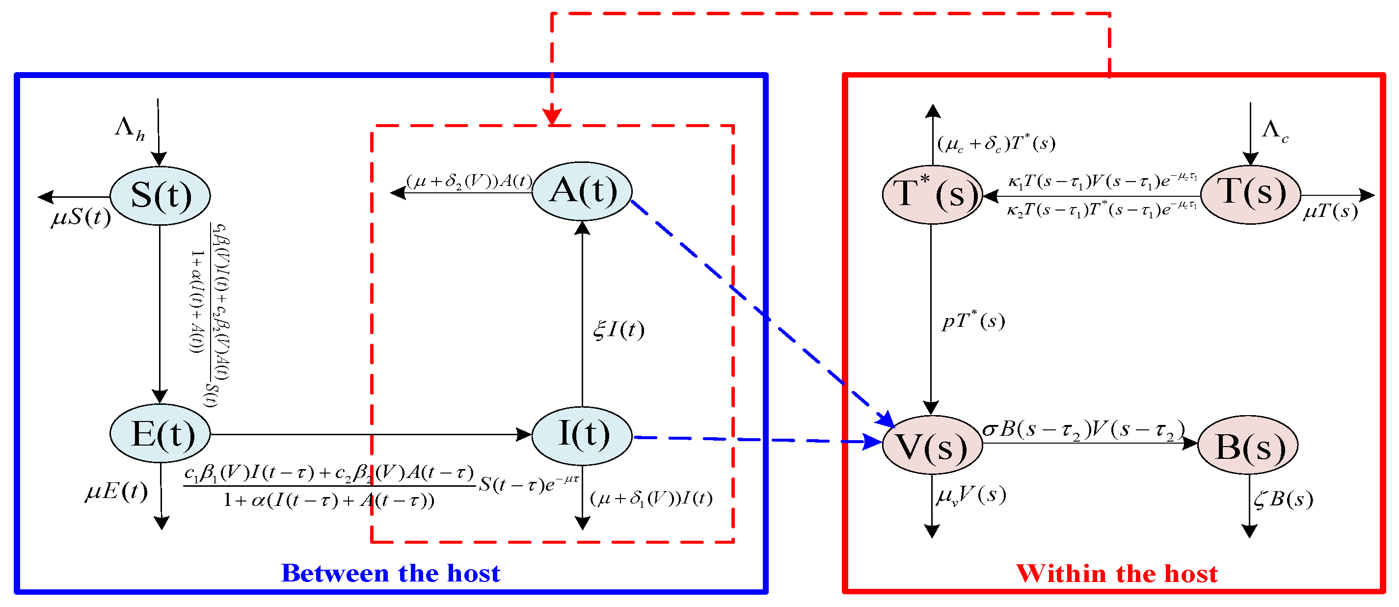
The flowchart of Model (1) and Model (2) are shown by the Figure 1. In addition, the multiscale model is characterized by two distinct time scales, denoted by t and s, respectively. The former represents the transmission time at the population level, while the latter represents the evolution time at the individual host level. Typically, the virus–cell dynamics within the host occur on a faster time scale than those between hosts. Therefore, s is a faster time scale than t (see [29,30,31]). Without loss of generality, we suppose that s = ϵ t ( 0 < ϵ 1 ) , where ϵ is a small positive constant.
Since the second equation of Model (1) is decoupled from the other equations, in the analysis below, it suffices to study the following between-host model
d S ( t ) d t = Λ h c 1 β 1 ( V ( s ) ) I ( t ) + c 2 β 2 ( V ( s ) ) A ( t ) 1 + α ( I ( t ) + A ( t ) ) S ( t ) μ S ( t ) , d I ( t ) d t = c 1 β 1 ( V ( s ) ) I ( t τ ) + c 2 β 2 ( V ( s ) ) A ( t τ ) 1 + α ( I ( t τ ) + A ( t τ ) ) S ( t τ ) e μ τ ( μ + ξ + δ 1 ( V ( s ) ) ) I ( t ) , d A ( t ) d t = ξ I ( t ) ( μ + δ 2 ( V ( s ) ) ) A ( t ) .

3. Analysis of the Fast Time Model

In the fast time Model (2), assume that, for HIV-positive individuals, I ( t ) is a constant I and, for AIDS individuals, A ( t ) is a constant A, where I = A = 0 means there is no possibility of viral transmission through direct contact with infected individuals, and I, A > 0 represent that the virus in the process of contacting infected individuals. And we denote c 1 η 1 I + c 2 η 2 A 1 + α ( I + A ) : = Θ ( I , A ) . Hence, Model (2) becomes the following isolated within-host virus infection model
d T ( s ) d s = Λ c κ 1 T ( s ) V ( s ) κ 2 T ( s ) T * ( s ) μ c T ( s ) , d T * ( s ) d s = ( κ 1 T ( s τ 1 ) V ( s τ 1 ) + κ 2 T ( s τ 1 ) T * ( s τ 1 ) ) e μ c τ 1 ( μ c + δ c ) T * ( s ) , d V ( s ) d s = Θ ( I , A ) + p T * ( s ) q B ( s ) V ( s ) μ v V ( s ) , d B ( s ) d s = σ B ( s τ 2 ) V ( s τ 2 ) ζ B ( s ) .
Let τ max = max { τ 1 , τ 2 } > 0 , then we define C ( [ τ max , 0 ] , R + 4 ) , equipped with the suitable sup-norm, as the Banach space of all continuous functions ϕ = ( ϕ 1 , ϕ 2 , ϕ 3 , ϕ 4 ) : [ τ max , 0 ] R + 4 . From the biological background of Model (4), the initial condition for any solution is given by
T ( ϑ ) = ϕ 1 ( ϑ ) , T * ( ϑ ) = ϕ 2 ( ϑ ) , V ( ϑ ) = ϕ 3 ( ϑ ) , B ( ϑ ) = ϕ 4 ( ϑ ) , ϕ i ( ϑ ) 0 , ϑ [ τ max , 0 ] , ϕ 1 ( 0 ) > 0 , i = 1 , 2 , 3 , 4 ,
where ϕ C ( [ τ max , 0 ] , R + 4 ) . It can be proved by the fundamental theory of functional differential equations [35] that Model (4) has the unique solution ( T ( s ) , T * ( s ) , V ( s ) , B ( s ) ) that satisfies the initial condition (5). Regarding the nonnegativity and boundedness of solutions for Model (4), we can state the following result.
Theorem 1.
Under the initial condition (5), the solution ( T ( s ) , T * ( s ) , V ( s ) , B ( s ) ) of Model (4) is nonnegative and bounded for all s 0 .
Following the approach in [21], the proof of nonnegativity and boundedness of solutions is straightforward and is omitted here.
Remark 3.
Theorem 1 indicates that the biologically feasible region
Ω = ( T , T * , V , B ) R + 4 : T + e μ c τ 1 T * Λ c μ c , V + q σ B p Λ c + e μ c τ 1 μ c Θ ( I , A ) e μ c τ 1 μ c min { μ v , ζ }
is positively invariant for Model (4). Therefore, in what follows, we only consider the solutions with initial conditions within the region Ω.

3.1. Feasible Equilibria and Basic Reproduction Number

In this section, we are dedicated to exploring the existence of equilibria and the reproduction number for Model (4). For I = A = 0 , the immune-inactivated reproduction number, R 0 w , and the immune-activated reproduction number, R 1 w , are defined, respectively, by
R 0 w = ( p κ 1 + μ v κ 2 ) Λ c μ c μ v ( μ c + δ c ) e μ c τ 1 , R 1 w = R 0 w 1 + μ v ( μ c + δ c ) ζ σ p Λ c e μ c τ 1 R 0 w .
The existence of equilibria of Model (4) in the case of I = A = 0 has been investigated in [21], and here we can summarize the following results.
Lemma 1.
Assume that I = A = 0 in Model (4), then the following statements are valid.
( i )
Model (4) always has infection-free equilibrium U 0 = ( T 0 , 0 , 0 , 0 ) , where T 0 = Λ c / μ c .
( i i )
If R 0 w > 1 , Model (4) has an immunity-inactivated infection equilibrium U 1 = ( T 1 , T 1 * , V 1 , 0 ) , where
T 1 = T 0 R 0 w , T 1 * = μ v μ c κ 1 p + κ 2 μ v ( R 0 w 1 ) , V 1 = p μ c κ 1 p + κ 2 μ v ( R 0 w 1 ) .
( i i i )
If R 1 w > 1 , except for U 0 and U 1 , Model (4) also has an immunity-activated infection equilibrium U 2 = ( T 2 , T 2 * , V 2 , B 2 ) , where
T 2 = Λ c κ 1 V 2 + κ 2 T 2 * + μ c , T 2 * = q ζ p σ B 2 + μ v ζ p σ , V 2 = ζ σ ,
and B 2 is the positive real root of the following equation
B 2 2 + 2 κ 2 ζ μ v + κ 1 ζ p + σ μ c μ v κ 2 ζ q σ p Λ c e μ c τ 1 ( μ c + δ c ) ζ q B 2 + κ 2 ζ μ v 2 + κ 1 ζ p μ v + σ μ c p μ v κ 2 ζ q 2 ( 1 R 1 w ) = 0 .
For I, A > 0 , Model (4) has no infection-free equilibrium, and the immune-activated reproduction number for Model (4) is defined by
R w = 2 σ Θ ( I , A ) + σ p b 1 + b 1 2 4 b 2 2 μ v ζ ,
where
b 1 = ( μ c + δ c ) ( κ 1 ζ + μ c σ ) e μ c τ 1 Λ c κ 2 σ κ 2 ( μ c + δ c ) σ e μ c τ 1 , b 2 = Λ c κ 1 ζ κ 2 ( μ c + δ c ) σ e μ c τ 1 .
The existence of equilibria for Model (4) in the scenario where I , A > 0 can be obtained based on the reproduction number R w , as shown below.
Theorem 2.
Assume that I , A > 0 in Model (4), the following statements are valid.
( i )
If R w 1 , Model (4) only has an immunity-inactivated infection equilibrium U ˜ 1 ( T ˜ 1 , T ˜ 1 * , V ˜ 1 , 0 ) , where T ˜ 1 , T ˜ 1 * , and V ˜ 1 are given below. Furthermore,
lim A , I 0 + U ˜ 1 ( T ˜ 1 , T ˜ 1 * , V ˜ 1 , 0 ) = U 0 ( T 0 , 0 , 0 , 0 ) , R 0 w 1 , U 1 ( T 1 , T 1 * , V 1 , 0 ) , R 0 w > 1 .
( i i )
If R w > 1 , except for U ˜ 1 , Model (4) also has a unique immunity-activated infection equilibrium, U ˜ 2 ( T ˜ 2 , T ˜ 2 * , V ˜ 2 , B ˜ 2 ) , where T ˜ 2 , T ˜ 2 * , V ˜ 2 , and B ˜ 2 are given below. Furthermore,
lim A , I 0 + U ˜ 2 ( T ˜ 2 , T ˜ 2 * , V ˜ 2 , B ˜ 2 ) = U 0 ( T 0 , 0 , 0 , 0 ) , R 0 w 1 , U 1 ( T 1 , T 1 * , V 1 , 0 ) , R 0 w > 1 , R 1 w 1 , U 2 ( T 2 , T 2 * , V 2 , B 2 ) , R 0 w > 1 , R 1 w > 1 .
Proof. 
Firstly, when I, A > 0 , the equilibrium U ˜ 1 = ( T ˜ 1 , T ˜ 1 * , V ˜ 1 , 0 ) satisfies the following equations
Λ c κ 1 T ˜ 1 V ˜ 1 κ 2 T ˜ 1 T ˜ 1 * μ c T ˜ 1 = 0 , ( κ 1 T ˜ 1 V ˜ 1 + κ 2 T ˜ 1 T ˜ 1 * ) e μ c τ 1 ( μ c + δ c ) T ˜ 1 * = 0 , Θ ( I , A ) + p T ˜ 1 * μ v V ˜ 1 = 0 .
We directly obtain
T ˜ 1 * = ( Λ c μ c T ˜ 1 ) e μ c τ 1 μ c + δ c , V ˜ 1 = Θ ( I , A ) + p T ˜ 1 * μ v ,
and T ˜ 1 is a solution of the following quadratic equation
T ˜ 1 2 + a 1 T ˜ 1 + a 2 = 0 ,
where a 1 = T 0 1 + 1 R 0 w + κ 1 Θ ( I , A ) μ v μ c R 0 w < 0 , a 2 = T 0 2 R 0 w > 0 . By calculation, Equation (8) has two real roots
T ˜ 1 + = 1 2 a 1 + a 1 2 4 a 2 > 0 , T ˜ 1 = 1 2 a 1 a 1 2 4 a 2 > 0 ,
with a 1 2 4 a 2 > 0 . Further, it is easy to verify T ˜ 1 + > Λ c μ c > T ˜ 1 . Hence, Model (4) has a unique immunity-inactivated infection equilibrium, U ˜ 1 = ( T ˜ 1 , T ˜ 1 * , V ˜ 1 , 0 ) , with
T ˜ 1 = 1 2 a 1 a 1 2 4 a 2 , V ˜ 1 = Θ ( I , A ) ( μ c + δ c ) + p ( Λ c μ c T ˜ 1 ) e μ c τ 1 μ v ( μ c + δ c ) , T ˜ 1 * = ( Λ c μ c T ˜ 1 ) e μ c τ 1 μ c + δ c .
Secondly, when I, A > 0 , we obtain
T ˜ 2 = Λ c ( μ c + δ c ) T ˜ 2 * e μ c τ 1 μ c , V ˜ 2 = ζ σ ,
and T ˜ 2 * satisfies T ˜ 1 * 2 + b 1 T ˜ 1 * + b 2 = 0 . Solving this equation, we obtain two real roots
T ˜ 2 + * = 1 2 b 1 + b 1 2 4 b 2 > 0 , T ˜ 2 * = 1 2 b 1 b 1 2 4 b 2 < 0 ,
with b 1 2 4 b 2 > 0 . For the positive equilibrium, U ˜ 2 , it should satisfy T ˜ 2 , T ˜ 2 * , V ˜ 2 , B ˜ 2 > 0 . Thus, if R w > 1 , Model (4) has a unique immunity-activated infection equilibrium, U ˜ 2 = ( T ˜ 2 , T ˜ 2 * , V ˜ 2 , B ˜ 2 ) , with
V ˜ 2 = ζ σ , T ˜ 2 * = 1 2 b 1 + b 1 2 4 b 2 , T ˜ 2 = Λ c κ 1 V ˜ 2 + κ 2 T ˜ 2 * + μ c , B ˜ 2 = 2 σ Θ ( I , A ) + σ p b 1 + b 1 2 4 b 2 2 μ v ζ 2 q ζ .
The proof is finished. □

3.2. Stability of Equilibria and Hopf Bifurcation

In this section, we with the global asymptotic stability of feasible equilibria and the existence of Hopf bifurcation of Model (4). To facilitate our discussion, we introduce the function ρ ( x ) = x 1 ln x . Note that ρ ( x ) 0 for x > 0 and d ρ ( x ) d x = 1 1 x . Moreover, ρ ( x ) = 0 if and only if x = 1 . On the global asymptotic stability of U ˜ 1 and U ˜ 2 , the following result is established.
Theorem 3.
Let I, A > 0 in Model (4),
( i )
if R w 1 , the immunity-inactivated equilibrium, U ˜ 1 , is globally asymptotically stable;
( i i )
if R w > 1 and τ 2 = 0 , the immunity-activated infection equilibrium, U ˜ 2 , is globally asymptotically stable.
Proof. 
We focus, firstly, the stability of equilibrium U ˜ 1 . To this end, we choose
L 1 ( s ) = T ˜ 1 ρ T ( s ) T ˜ 1 + e μ c τ 1 T ˜ 1 * ρ T * ( s ) T ˜ 1 * + κ 1 T ˜ 1 V ˜ 1 p T ˜ 1 * V ˜ 1 ρ V ( s ) V ˜ 1 + κ 1 T ˜ 1 V ˜ 1 s τ 1 s ρ T ( x 1 ) V ( x 1 ) T ˜ 1 V ˜ 1 d x 1 + q κ 1 T ˜ 1 V ˜ 1 σ p T ˜ 1 * B ( s ) + κ 2 T ˜ 1 T ˜ 1 * s τ 1 s ρ T ( x 1 ) T * ( x 1 ) T ˜ 1 T ˜ 1 * d x 1 + q κ 1 T ˜ 1 V ˜ 1 p T ˜ 1 * s τ 2 s B ( x 1 ) V ( x 1 ) d x 1 .
Calculating the time derivative of L 1 ( s ) along the positive solution of Model (4) yields
d L 1 ( s ) d s = κ 1 T ˜ 1 V ˜ 1 ρ T ˜ 1 T ( s ) κ 1 T ˜ 1 V ˜ 1 ρ T * ( s ) V ˜ 1 T ˜ 1 * V ( s ) κ 1 T ˜ 1 V ˜ 1 ρ T ( s τ 1 ) V ( s τ 1 ) T ˜ 1 * T ˜ 1 V ˜ 1 T * ( s ) κ 2 T ˜ 1 T ˜ 1 * ρ T ˜ 1 T ( s ) κ 2 T ˜ 1 T ˜ 1 * ρ T ( s τ 1 ) T * ( s τ 1 ) T ˜ 1 T * ( s ) + ζ q κ 1 T ˜ 1 V ˜ 1 σ p T ˜ 1 * R w 1 B ( s ) μ c ( T ( s ) T ˜ 1 ) 2 T ( s ) + κ 1 T ˜ 1 V ˜ 1 p T ˜ 1 * Θ ( I , A ) 2 V ( s ) V ˜ 1 V ˜ 1 V ( s ) .
Therefore, under the assumption R w 1 , we have d L 1 ( s ) d s 0 . Additionally, it can be easily verified that T ( s ) = T ˜ 1 , T * ( s ) = T ˜ 1 * , V ( s ) = V ˜ 1 , and B ( s ) = 0 when d L 1 ( s ) d s = 0 . Consequently, the singleton { U ˜ 1 } is the largest compact invariant set in { ( T ( s ) , T * ( s ) , B ( s ) , V ( s ) ) R + 4 : d L 1 ( s ) d s = 0 } . Therefore, by applying LaSalle’s invariance principle, the immunity-inactivated infection equilibrium, U ˜ 1 , is globally asymptotically stable when R w 1 .
Now, we turn to the conclusion ( i i ) . For equilibrium U ˜ 2 , one defines
L 2 ( s ) = T ˜ 2 ρ T ( s ) T ˜ 2 + e μ c τ 1 T ˜ 2 * ρ T * ( s ) T ˜ 2 * + κ 1 T ˜ 2 V ˜ 2 p T ˜ 2 * V ˜ 2 ρ V ( s ) V ˜ 2 + q κ 1 T ˜ 2 V ˜ 2 σ P T ˜ 2 * B ˜ 2 ρ B ( s ) B ˜ 2 + κ 1 T ˜ 2 V ˜ 2 s τ 1 s ρ T ( x 1 ) V ( x 1 ) T ˜ 2 V ˜ 2 d x 1 + κ 2 T ˜ 2 T ˜ 2 * s τ 1 s ρ T ( x 1 ) T * ( x 1 ) T ˜ 2 T ˜ 2 * d x 1 .
Calculating the time derivative of L 2 ( s ) along the positive solution of Model (4) yields
d L 2 ( s ) d s = μ c ( T ( s ) T ˜ 2 ) 2 T ( s ) κ 1 T ˜ 2 V ˜ 2 ρ T ˜ 2 T ( s ) κ 1 T ˜ 2 V ˜ 2 ρ T * ( s ) V ˜ 2 T ˜ 2 * V ( s ) κ 1 T ˜ 2 V ˜ 2 ρ T ( s τ 1 ) V ( s τ 1 ) T ˜ 2 * T ˜ 2 V ˜ 2 T * ( s ) κ 2 T ˜ 2 T ˜ 2 * ρ T ˜ 2 T ( s ) κ 2 T ˜ 2 T ˜ 2 * ρ T ( s τ 1 ) T * ( s τ 1 ) T ˜ 2 T * ( s ) + κ 1 T ˜ 2 V ˜ 2 p T ˜ 2 * Θ ( I , A ) 2 V ( s ) V ˜ 2 V ˜ 2 V ( s ) .
Thus, we have d L 2 ( s ) d s 0 , and equality holds if and only if T ( s ) = T ˜ 2 , T * ( s ) = T ˜ 2 * , V ( s ) = V ˜ 2 , and B ( s ) = B ˜ 2 . Consequently, the singleton { U ˜ 2 } is the largest compact invariant set in { ( T ( s ) , T * ( s ) , B ( s ) , V ( s ) ) R + 4 : d L 2 ( s ) d s = 0 } . Therefore, by applying LaSalle’s invariance principle, the immunity-activated equilibrium, U ˜ 2 , is globally asymptotically stable when R w > 1 and τ 2 = 0 . □
Remark 4.
For Model (4) with I = A = 0 , it is easy to verify the global asymptotic stability of U 0 , U 1 , and U 2 , respectively, by constructing
L 0 ( s ) = T 0 ρ T ( s ) T 0 + e μ c τ 1 T * ( s ) + κ 1 T 0 μ v V ( s ) + q κ 1 T 0 σ μ v B ( s ) + q κ 1 T 0 μ v s τ 2 s B ( x 1 ) V ( x 1 ) d x 1 + s τ 1 s κ 1 T ( x 1 ) V ( x 1 ) + κ 2 T ( x 1 ) T * ( x 1 ) d x 1
and same Lyapunov functionals as in Theorem 3. Thus we omit here.
Next, our focus is on examining the necessary and sufficient conditions for Hopf bifurcation to take place at U ˜ 2 . The characteristic equation of (4) at U ˜ 2 is
λ 4 + C ¯ 3 λ 3 + C ¯ 2 λ 2 + C ¯ 1 λ + C ¯ 0 + ( D ¯ 3 λ 3 + D ¯ 2 λ 2 + D ¯ 1 λ + D ¯ 0 ) e ( μ c + λ ) τ 1 + ( E ¯ 3 λ 3 + E ¯ 2 λ 2 + E ¯ 1 λ + E ¯ 0 ) e λ τ 2 + ( F ¯ 2 λ 2 + F ¯ 1 λ + F ¯ 0 ) e μ c τ 1 ( τ 1 + τ 2 ) λ = 0 ,
where
C ¯ 3 = κ 1 V ˜ 2 + κ 2 T ˜ 2 * + 2 μ c + δ c + q B ˜ 2 + μ v + ζ , E ¯ 1 = σ V ˜ 2 ( μ c + δ c ) ( κ 1 V ˜ 2 + κ 2 T ˜ 2 * + μ c ) σ V ˜ 2 μ v ( κ 1 V ˜ 2 + κ 2 T ˜ 2 * + 2 μ c + δ c ) , C ¯ 2 = ( κ 1 V ˜ 2 + κ 2 T ˜ 2 * + μ c ) ( μ c + δ c ) + ( κ 1 V ˜ 2 + κ 2 T ˜ 2 * + 2 μ c + δ c ) ( q B ˜ 2 + μ v + ζ ) + ζ ( q B ˜ 2 + μ v ) , C ¯ 1 = ( q B ˜ 2 + μ v + ζ ) ( κ 1 V ˜ 2 + κ 2 T ˜ 2 * + μ c ) ( μ c + δ c ) + ζ ( q B ˜ 2 + μ v ) ( κ 1 V ˜ 2 + κ 2 T ˜ 2 * + 2 μ c + δ c ) , C ¯ 0 = ζ ( q B ˜ 2 + μ v ) ( κ 1 V ˜ 2 + κ 2 T ˜ 2 * + μ c ) ( μ c + δ c ) , D ¯ 3 = κ 2 T ˜ 2 , D ¯ 2 = κ 2 T ˜ 2 ( μ c + q B ˜ 2 + μ v + ζ ) p κ 1 T ˜ 2 , D ¯ 1 = κ 2 T ˜ 2 μ c ( q B ˜ 2 + μ v + ζ ) p κ 1 T ˜ 2 ( μ c + ζ ) ζ κ 2 T ˜ 2 ( q B ˜ 2 + μ v ) , D ¯ 0 = ζ κ 2 T ˜ 2 μ c ( q B ˜ 2 + μ v ) ζ p κ 1 T ˜ 2 μ c , E ¯ 3 = σ V ˜ 2 , E ¯ 2 = σ V 2 ( κ 1 V ˜ 2 + κ 2 T ˜ 2 * + 2 μ c + δ c + μ v ) , E ¯ 0 = σ V ˜ 2 μ c ( κ 1 V ˜ 2 + κ 2 T ˜ 2 * + μ c ) ( μ c + δ c ) , F ¯ 2 = σ V ˜ 2 κ 2 T ˜ 2 * , F ¯ 1 = σ V ˜ 2 κ 2 T ˜ 2 ( μ c + μ v ) + σ V ˜ 2 p κ 1 T ˜ 2 , F ¯ 0 = σ V ˜ 2 T ˜ 2 μ c ( κ 2 μ v + κ 1 p ) .
For τ 2 > 0 , we will categorize the stability analysis of U ˜ 2 into two cases, respectively.
Case 1:
τ 1 = 0 and τ 2 > 0 .
Equation (9) is, in this case, reduced to
λ 4 + P ¯ 3 λ 3 + P ¯ 2 λ 2 + P ¯ 1 λ + P ¯ 0 + ( Q ¯ 3 λ 3 + Q ¯ 2 λ 2 + Q ¯ 1 λ + Q ¯ 0 ) e λ τ 2 = 0 ,
where P ¯ 3 = C ¯ 3 + D ¯ 3 , P ¯ 2 = C ¯ 2 + D ¯ 2 , P ¯ 1 = C ¯ 1 + D ¯ 1 , P ¯ 0 = C ¯ 0 + D ¯ 0 , Q ¯ 3 = E ¯ 3 , Q ¯ 2 = E ¯ 2 + F ¯ 2 , Q ¯ 1 = E ¯ 1 + F ¯ 1 , Q ¯ 0 = E ¯ 0 + F ¯ 0 . Let λ = i ω be a purely imaginary root of (10), and substituting λ = i ω into (10) and separating the real and imaginary parts, we obtain
( Q ¯ 3 ω 3 Q ¯ 1 ω ) sin ( ω τ 2 ) + ( Q ¯ 2 ω 2 Q ¯ 0 ) cos ( ω τ 2 ) = ω 4 P ¯ 2 ω 2 + P ¯ 0 , ( Q ¯ 3 ω 3 Q ¯ 1 ω ) cos ( ω τ 2 ) ( Q ¯ 2 ω 2 Q ¯ 0 ) sin ( ω τ 2 ) = P ¯ 3 ω 3 + P ¯ 1 ω .
Squaring and adding both above equations lead to the following equation
ω 8 + G ¯ 6 ω 6 + G ¯ 4 ω 4 + G ¯ 2 ω 2 + G ¯ 0 = 0 ,
where G ¯ 6 = P ¯ 3 2 Q ¯ 3 2 2 P ¯ 2 , G ¯ 4 = P ¯ 2 2 + 2 P ¯ 0 + 2 Q ¯ 1 Q ¯ 3 2 P ¯ 1 P ¯ 3 Q ¯ 2 2 , G ¯ 2 = P ¯ 1 2 + 2 Q ¯ 0 Q ¯ 2 2 P ¯ 0 P ¯ 2 Q ¯ 1 2 , G ¯ 0 = P ¯ 0 2 Q ¯ 0 2 . Let u = ω 2 , then (12) is equivalent to
f ( u ) = u 4 + G ¯ 6 u 3 + G ¯ 4 u 2 + G ¯ 2 u + G ¯ 0 = 0 .
If G ¯ 0 < 0 , then it can be observed that (13) must have at least one positive root. This is because the function f ( u ) satisfies f ( 0 ) = G ¯ 0 < 0 and lim u f ( u ) = + . Therefore, there exists a value u 0 ( 0 , + ) such that f ( u 0 ) = 0 . Furthermore,
f ( u ) = 4 u 3 + 3 G ¯ 6 u 2 + 2 G ¯ 4 u + G ¯ 2 .
Let v = u + 3 G ¯ 6 4 , then Equation (14) becomes v 3 + n 1 v + n 2 = 0 , where n 1 = 1 2 G ¯ 4 2 3 16 G ¯ 6 2 , n 2 = 1 32 G ¯ 6 3 1 8 G ¯ 6 G ¯ 4 + G ¯ 2 . Let Δ = ( n 2 2 ) 2 + ( n 1 3 ) 3 and j = 1 + i 3 2 , then
v 1 = n 2 2 + Δ 3 + n 2 2 Δ 3 , v 2 = j n 2 2 + Δ 3 + j 2 n 2 2 Δ 3 , v 3 = j 2 n 2 2 + Δ 3 + j n 2 2 Δ 3 , u i = v i 3 G ¯ 6 4 , i = 1 , 2 , 3 .
Applying the method described in [36], we can obtain the following result regarding the root distribution of Equation (13).
Lemma 2.
For polynomial Equation (13),
( i )
if G ¯ 0 < 0 , then Equation (13) has at least one positive root;
( i i )
if G ¯ 0 0 and Δ 0 , then Equation (13) has a positive root if and only if u 1 > 0 and f ( u 1 ) < 0 ;
( i i i )
if G ¯ 0 0 and Δ < 0 , then Equation (13) has a positive root if and only if there exists at least one u * { u 1 , u 2 , u 3 } , such that u * > 0 and f ( u * ) 0 .
If the conditions in Lemma 2 are invalid, then Equation (13) does not have any positive root. This implies that Equation (10) does not have purely imaginary roots. Furthermore, U ˜ 2 is locally asymptotically stable for all delay τ 2 0 . As a result, the existence of Hopf bifurcation is not possible.
We now assume that one of the conditions in Lemma 2, which guarantees the existence of positive roots for Equation (13), is true and that Equation (13) has k 0 ( 1 k 0 4 ) positive roots. Let u k , k = 1 , , k 0 be the positive roots of (13), then Equation (12) has positive roots ω k = u k . For a given ω k , the corresponding critical value of delay τ 2 is
τ 2 , k ( j ) = 1 ω k arccos ( ω k 4 P ¯ 2 ω k 2 + P ¯ 0 ) ( Q ¯ 2 ω k 2 Q ¯ 0 ) + ( P ¯ 3 ω k 3 + P ¯ 1 ω k ) ( Q ¯ 3 ω k 3 Q ¯ 1 ω k ) ( Q ¯ 3 ω k 3 Q ¯ 1 ω k ) 2 + ( Q ¯ 2 ω k 2 Q ¯ 0 ) 2 + 2 j π ω k ,
j = 0 , 1 , 2 , . Then ± i ω k are a pair of purely imaginary roots of (10) with τ 2 = τ 2 , k ( j ) . Define
τ 2 0 = τ 2 , k 0 ( 0 ) = min τ 2 , k ( j ) | k = 1 , 2 , , k 0 , j = 0 , 1 , , ω 0 = ω k 0 , u 0 = u k 0 .
Let λ ( τ ) = α ( τ ) + i ω ( τ ) be the root of Equation (10) at τ = τ 2 0 satisfying α ( τ 2 0 ) = 0 and ω ( τ 2 0 ) = ω 0 . Similar to the proof in [14], the transversality condition at τ 2 = τ 2 0 will be verified. Differentiating both sides of (10) with respect to τ 2 , we obtain
d λ d τ 2 1 = 4 λ 3 + 3 P ¯ 3 λ 2 + 2 P ¯ 2 λ + P ¯ 1 λ ( λ 4 + P ¯ 3 λ 3 + P ¯ 2 λ 2 + P ¯ 1 λ + P ¯ 0 ) + 3 Q ¯ 3 λ 2 + 2 Q ¯ 2 λ + Q ¯ 1 λ ( Q ¯ 3 λ 3 + Q ¯ 2 λ 2 + Q ¯ 1 λ + Q ¯ 0 ) τ 2 λ .
From Equation (11), one has
( Q ¯ 3 ω 0 3 Q ¯ 1 ω 0 ) 2 + ( Q ¯ 2 ω 0 2 Q ¯ 0 ) 2 = ( ω 0 4 P ¯ 2 ω 0 2 + P ¯ 0 ) 2 + ( P ¯ 1 ω 0 P ¯ 3 ω 0 3 ) 2 .
Then, evaluating d λ d τ 2 1 at τ 2 = τ 2 0 ( i . e . λ = i ω 0 ) and taking the real part, we obtain
Re d λ d τ 2 1 | τ 2 = τ 2 0 = 4 ω 0 6 + 3 G ¯ 6 ω 0 4 + 2 G ¯ 4 ω 0 2 + G ¯ 2 ( Q ¯ 3 ω 0 3 Q ¯ 1 ω 0 ) 2 + ( Q ¯ 2 ω 0 2 Q ¯ 0 ) 2 = f ( ω 0 2 ) ( Q ¯ 3 ω 0 3 Q ¯ 1 ω 0 ) 2 + ( Q ¯ 2 ω 0 2 Q ¯ 0 ) 2 .
Therefore,
sign d ( Re ( λ ) ) d τ 2 | τ 2 = τ 2 0 = sign Re d λ d τ 2 1 | τ 2 = τ 2 0 = sign { f ( ω 0 2 ) } = sign { f ( u 0 ) } .
Based on the aforementioned analysis and the Hopf bifurcation theorem presented in [37], we can conclude the following result.
Theorem 4.
If all the conditions in Lemma 2 are not satisfied, then U ˜ 2 is locally asymptotically stable for all τ 2 0 . If one of the conditions in Lemma 2 is satisfied, then U ˜ 2 is locally asymptotically stable for τ 2 within the interval [ 0 , τ 2 0 ) . If one of the conditions in Lemma 2 is satisfied and f ( u 0 ) 0 , then the transversality condition holds, and Model (4) will undergo a Hopf bifurcation at U ˜ 2 when τ 2 = τ 2 0 .
Case 2:
τ 1 > 0 and τ 2 > 0 .
We take τ 2 as the bifurcation parameter and assume the purely imaginary root of Equation (9) to be λ = i ω ˜ with ω ˜ > 0 . By following the same computational process, it is clear that
Π 1 cos ( ω ˜ τ 2 ) Π 2 sin ( ω ˜ τ 2 ) = Π 3 , Π 1 sin ( ω ˜ τ 2 ) + Π 2 cos ( ω ˜ τ 2 ) = Π 4 ,
where
Π 1 = E ¯ 2 ω ˜ 2 E ¯ 0 + ( F ¯ 2 ω ˜ 2 F ¯ 0 ) cos ( ω ˜ τ 1 ) e μ c τ 1 F ¯ 1 ω ˜ sin ( ω ˜ τ 1 ) e μ c τ 1 , Π 2 = E ¯ 1 ω ˜ E ¯ 3 ω ˜ 3 + ( F ¯ 2 ω ˜ 2 F ¯ 0 ) sin ( ω ˜ τ 1 ) e μ c τ 1 + F ¯ 1 ω ˜ cos ( ω ˜ τ 1 ) e μ c τ 1 , Π 3 = ω ˜ 4 C ¯ 2 ω ˜ 2 + C ¯ 0 + ( D ¯ 0 D ¯ 2 ω ˜ 2 ) cos ( ω ˜ τ 1 ) e μ c τ 1 + ( D ¯ 1 ω ˜ D ¯ 3 ω ˜ 3 ) sin ( ω ˜ τ 1 ) e μ c τ 1 , Π 4 = C ¯ 3 ω ˜ 3 C ¯ 1 ω ˜ + ( D ¯ 3 ω ˜ 3 D ¯ 1 ω ˜ ) cos ( ω ˜ τ 1 ) e μ c τ 1 + ( D ¯ 0 D ¯ 2 ω ˜ 2 ) sin ( ω ˜ τ 1 ) e μ c τ 1 .
From (15), one has
Ϝ 1 ( ω ˜ ) + Ϝ 2 ( ω ˜ ) cos ( ω ˜ τ 1 ) + Ϝ 3 ( ω ˜ ) sin ( ω ˜ τ 1 ) = 0 ,
where
Ϝ 1 ( ω ˜ ) = C ¯ 1 2 + E ¯ 1 2 + 2 C ¯ 0 C ¯ 2 2 E ¯ 0 E ¯ 2 D ¯ 1 2 e 2 μ c τ 1 + F ¯ 1 2 e 2 μ c τ 1 + 2 D ¯ 0 D ¯ 2 e 2 μ c τ 1 2 F ¯ 0 F ¯ 2 e 2 μ c τ 1 ω ˜ 2 + 2 C ¯ 0 C ¯ 2 2 + E ¯ 2 2 + 2 C ¯ 1 C ¯ 3 2 E ¯ 1 E ¯ 3 D ¯ 2 2 e 2 μ c τ 1 + F ¯ 2 2 e 2 μ c τ 1 + 2 D ¯ 1 D ¯ 3 e 2 μ c τ 1 ω ˜ 4 + ω ˜ 8 + 2 C ¯ 2 + E ¯ 3 2 C ¯ 3 2 D ¯ 3 2 e 2 μ c τ 1 ω ˜ 6 + E ¯ 0 2 C ¯ 0 2 + F ¯ 0 2 e 2 μ c τ 1 D ¯ 0 2 e 2 μ c τ 1 , Ϝ 2 ( ω ˜ ) = ( 2 D ¯ 2 2 C ¯ 3 D ¯ 3 ) e 2 μ c τ 1 ω ˜ 6 + 2 D ¯ 0 2 C ¯ 1 D ¯ 3 2 C ¯ 2 D ¯ 2 + 2 C ¯ 3 D ¯ 1 + 2 E ¯ 2 F ¯ 2 2 E ¯ 3 F ¯ 1 e 2 μ c τ 1 ω ˜ 4 + 2 C ¯ 0 D ¯ 2 2 C ¯ 1 D ¯ 1 + 2 C ¯ 2 D ¯ 0 2 E ¯ 0 F ¯ 2 + 2 E ¯ 1 F ¯ 1 2 E ¯ 2 F ¯ 0 e 2 μ c τ 1 ω ˜ 2 + 2 E ¯ 0 F ¯ 0 2 C ¯ 0 D ¯ 0 e 2 μ c τ 1 , Ϝ 3 ( ω ˜ ) = 2 D ¯ 3 e 2 μ c τ 1 ω ˜ 7 + 2 C ¯ 0 D ¯ 3 2 C ¯ 1 D ¯ 2 + 2 C ¯ 2 D ¯ 1 2 C ¯ 3 D ¯ 0 + 2 E ¯ 1 F ¯ 2 2 E ¯ 2 F ¯ 1 + 2 E ¯ 3 F ¯ 0 e 2 μ c τ 1 ω ˜ 3 + 2 D ¯ 1 2 C ¯ 2 D ¯ 3 + 2 C ¯ 3 D ¯ 2 2 E ¯ 3 F ¯ 2 e 2 μ c τ 1 ω ˜ 5 + 2 C ¯ 1 D ¯ 0 2 C ¯ 0 D ¯ 1 + 2 E ¯ 0 F ¯ 1 2 E ¯ 1 F ¯ 0 e 2 μ c τ 1 ω ˜ .
Denote Γ ( ω ˜ ) = Ϝ 1 ( ω ˜ ) + Ϝ 2 ( ω ˜ ) cos ( ω ˜ τ 1 ) + Ϝ 3 ( ω ˜ ) sin ( ω ˜ τ 1 ) . Obviously, lim ω ˜ + Γ ( ω ˜ ) = + . Further, if ( E ¯ 0 + F ¯ 0 ) 2 ( C ¯ 0 + D ¯ 0 ) 2 e 2 μ c τ 1 + ( E ¯ 0 2 C ¯ 0 2 ) ( 1 e 2 μ c τ 1 ) < 0 , that is, Γ ( 0 ) < 0 , then Equation (16) has k ˜ 0 ( 1 k ˜ 0 8 ) positive roots ω ˜ k . For each ω ˜ k , there is a corresponding critical value of delay τ 2 shown as
τ 2 , k ( j ) = 1 ω ˜ k arccos Π 1 Π 3 + Π 2 Π 4 Π 1 2 + Π 2 2 + 2 j π ω ˜ k , j = 0 , 1 , 2 , .
Let τ 2 * = τ 2 , k ˜ 0 ( 0 ) = min τ 2 , k ˜ ( j ) | k ˜ = 1 , 2 , , k ˜ 0 , j = 0 , 1 , , and let ω ˜ 0 = ω ˜ k ˜ 0 be the root of (9) with τ 2 * . Differentiating both sides of (9) with respect to τ 2 , we obtain
d λ d τ 2 1 = 4 λ 3 + 3 C ¯ 3 λ 2 + 2 C ¯ 2 λ + C ¯ 1 + ( 3 D ¯ 3 λ 2 + 2 D ¯ 2 λ + D ¯ 1 ) τ 1 ( D ¯ 3 λ 3 + D ¯ 2 λ 2 + D ¯ 1 λ + D ¯ 0 ) E λ λ 4 + C ¯ 3 λ 3 + C ¯ 2 λ 2 + C ¯ 1 λ + C ¯ 0 + ( D ¯ 3 λ 3 + D ¯ 2 λ 2 + D ¯ 1 λ + D ¯ 0 ) E + 2 E ¯ 3 λ 2 + 2 E ¯ 2 λ + E ¯ 1 + [ 2 F ¯ 2 λ + F ¯ 1 τ 1 ( F ¯ 2 λ 2 + F ¯ 1 λ + F ¯ 0 ) ] E λ [ E ¯ 3 λ 3 + E ¯ 2 λ 2 + E ¯ 1 λ + E ¯ 0 + ( F ¯ 2 λ 2 + F ¯ 1 λ + F ¯ 0 ) E ] τ 2 λ ,
where E = e ( μ c + λ ) τ 1 . Then evaluating d λ d τ 2 1 at τ 2 = τ 2 * ( i . e . λ = i ω ˜ 0 ) and taking the real part, one has
Re d λ d τ 2 1 | τ 2 = τ 2 * = C 11 + D 11 + E 11 + F 11 A 11 2 + B 11 2 ,
where
A 11 = C ¯ 3 ω ˜ 0 4 C ¯ 1 ω ˜ 0 2 + ( D ¯ 3 ω ˜ 0 4 D ¯ 1 ω ˜ 0 2 ) e μ c τ 1 cos ( ω ˜ 0 τ 1 ) + ( D ¯ 0 ω ˜ 0 D ¯ 2 ω ˜ 0 3 ) e μ c τ 1 sin ( ω ˜ 0 τ 1 ) , B 11 = ω ˜ 0 5 C ¯ 2 ω ˜ 0 3 + C ¯ 0 ω ˜ ( D ¯ 3 ω ˜ 0 4 D ¯ 1 ω ˜ 0 2 ) e μ c τ 1 sin ( ω ˜ 0 τ 1 ) + ( D ¯ 0 ω ˜ 0 D ¯ 2 ω ˜ 0 3 ) e μ c τ 1 cos ( ω ˜ 0 τ 1 ) , C 11 = 3 E ¯ 3 ω ˜ 0 2 + E ¯ 1 + [ F ¯ 1 τ 1 ( F ¯ 0 F ¯ 2 ω ˜ 0 2 ) ] e μ c τ 1 cos ( ω ˜ 0 τ 1 ) + ( 2 F ¯ 2 ω ˜ 0 τ 1 F ¯ 2 ω ˜ 0 ) e μ c τ 1 sin ( ω ˜ 0 τ 1 ) × E ¯ 3 ω ˜ 0 4 E ¯ 1 ω ˜ 0 2 F ¯ 1 ω ˜ 0 2 e μ c τ 1 cos ( ω ˜ 0 τ 1 ) + ( F ¯ 0 ω ˜ 0 F ¯ 2 ω ˜ 0 3 ) e μ c τ 1 sin ( ω ˜ 0 τ 1 ) , D 11 = 2 E ¯ 2 ω ˜ 0 + ( 2 F ¯ 2 ω ˜ 0 τ 1 F ¯ 1 ω ˜ 0 ) e μ c τ 1 cos ( ω ˜ 0 τ 1 ) + [ τ 1 ( F ¯ 0 F ¯ 2 ω ˜ 0 2 ) F ¯ 1 ] e μ c τ 1 sin ( ω ˜ 0 τ 1 ) × E ¯ 0 ω ˜ 0 E ¯ 2 ω ˜ 0 3 + ( F ¯ 0 ω ˜ 0 F ¯ 2 ω ˜ 0 3 ) e μ c τ 1 cos ( ω ˜ 0 τ 1 ) + F ¯ 1 ω ˜ 0 2 e μ c τ 1 sin ( ω ˜ 0 τ 1 ) , E 11 = { 3 E ¯ 3 ω ˜ 0 2 C ¯ 1 + [ 3 D ¯ 3 ω ˜ 0 2 D ¯ 1 + τ 1 ( D ¯ 0 D ¯ 2 ω ˜ 0 2 ) ] e μ c τ 1 cos ( ω ˜ 0 τ 1 ) + [ τ 1 ( D ¯ 1 ω ˜ 0 D ¯ 3 ω ˜ 0 3 ) 2 D ¯ 2 ω ˜ 0 ] e μ c τ 1 × sin ( ω ˜ 0 τ 1 ) } C ¯ 3 ω ˜ 0 4 C ¯ 1 ω ˜ 0 2 + ( D ¯ 3 ω ˜ 0 4 D ¯ 1 ω ˜ 0 2 ) e μ c τ 1 cos ( ω ˜ 0 τ 1 ) + ( D ¯ 0 ω ˜ 0 D ¯ 2 ω ˜ 0 3 ) e μ c τ 1 sin ( ω ˜ 0 τ 1 ) , F 11 = { 4 ω ˜ 0 3 2 C ¯ 2 ω ˜ 0 + [ τ 1 ( D ¯ 1 ω ˜ 0 D ¯ 3 ω ˜ 0 3 ) 2 D ¯ 2 ω ˜ 0 ] e μ c τ 1 cos ( ω ˜ 0 τ 1 ) + [ τ 1 ( D ¯ 2 ω ˜ 0 2 D ¯ 0 ) + D ¯ 1 3 D ¯ 3 ω ˜ 0 2 ] e μ c τ 1 × sin ( ω ˜ 0 τ 1 ) } [ ω ˜ 0 5 C ¯ 2 ω ˜ 0 3 + C ¯ 0 ω ˜ ( D ¯ 3 ω ˜ 0 4 D ¯ 1 ω ˜ 0 2 ) e μ c τ 1 sin ( ω ˜ 0 τ 1 ) + ( D ¯ 0 ω ˜ 0 D ¯ 2 ω ˜ 0 3 ) e μ c τ 1 cos ( ω ˜ 0 τ 1 ) ] .
Therefore,
sign d ( Re ( λ ) ) d τ 2 | τ 2 = τ 2 * = sign Re d λ d τ 2 1 | τ 2 = τ 2 * = sign C 11 + D 11 + E 11 + F 11 .
Based on the above arguments, we can derive the following results.
Theorem 5.
For Model (4), given that τ 1 > 0 and τ 2 > 0 , if Γ ( 0 ) < 0 and sign { C 11 + D 11 + E 11 + F 11 } 0 , then U ˜ 2 is locally asymptotically stable for all τ 2 [ 0 , τ 2 * ) , and unstable for τ 2 > τ 2 * . Additionally, Model (4) undergoes a Hopf bifurcation at U ˜ 2 when τ 2 = τ 2 * .

3.3. Direction and Stability of the Hopf Bifurcation

In this section, we will employ the standard form theory and the central manifold theorem presented in [38] to analyze the direction of the Hopf bifurcation and investigate the stability of the bifurcating periodic solution in Model (4) with respect to τ 2 . It is always assumed that Model (4) undergoes a Hopf bifurcation at U ˜ 2 when τ 1 > 0 and τ 2 = τ 2 * . Based on the biological context, it is useful to assume that τ 1 < τ 2 * , where τ 2 [ 0 , τ 2 * ) .
Let τ 2 = τ 2 * + μ ˜ , μ ˜ R , then Model (4) will generate Hopf bifurcation at U ˜ 2 when μ ˜ = 0 . Denote x ˜ ( s ) = ( x ˜ 1 ( s ) , x ˜ 2 ( s ) , x ˜ 3 ( s ) , x ˜ 4 ( s ) ) T R 4 , x ˜ 1 ( s ) = T T ˜ 2 , x ˜ 2 ( s ) = T * T ˜ 2 * , x ˜ 3 ( s ) = V V ˜ 2 , x ˜ 4 ( s ) = B B ˜ 2 , normalizing the delay s ( s τ 2 ) , then Model (4) can be transformed into
d x ˜ ( s ) d s = L μ ˜ ( x ˜ s ) f ( μ ˜ , x ˜ s ) ,
where maps L μ ˜ : C R 4 and f : R × C R 4 , respectively, are given by
L μ ˜ ( ϕ ) = ( τ 2 * + μ ˜ ) N 1 ϕ ( 0 ) + N 2 ϕ τ 1 τ 2 * + N 3 ϕ ( 1 ) , f ( μ ˜ , ϕ ) = ( τ 2 * + μ ˜ ) κ 1 ϕ 1 ( 0 ) ϕ 3 ( 0 ) κ 2 ϕ 1 ( 0 ) ϕ 2 ( 0 ) κ 1 e μ c τ 1 ϕ 1 τ 1 τ 2 * ϕ 3 τ 1 τ 2 * + κ 2 e μ c τ 1 ϕ 1 τ 1 τ 2 * ϕ 2 τ 1 τ 2 * q ϕ 3 ( 0 ) ϕ 4 ( 0 ) σ ϕ 3 ( 1 ) ϕ 4 ( 1 ) ,
where ϕ ( θ ) = ( ϕ 1 ( θ ) , ϕ 2 ( θ ) , ϕ 3 ( θ ) , ϕ 4 ( θ ) ) C , and
N 1 = κ 1 V ˜ 2 κ 2 T ˜ 2 * μ c κ 2 T ˜ 2 * κ 1 V ˜ 2 0 0 ( μ h + δ c ) 0 0 0 p q B ˜ 2 μ v q V ˜ 2 0 0 0 ζ ,
N 2 = 0 0 0 0 ( κ 1 V ˜ 2 + κ 2 T ˜ 2 * ) e μ c τ 1 κ 2 T ˜ 2 e μ c τ 1 κ 1 T ˜ 2 e μ c τ 1 0 0 0 0 0 0 0 0 0 , N 3 = 0 0 0 0 0 0 0 0 0 0 0 0 0 0 σ B ˜ 2 σ V ˜ 2 .
Hence, from the Riesz representation theorem, there is a 4 × 4 matrix function η ( θ , μ ˜ ) : [ 1 , 0 ] R 3 whose components are bounded, such that L μ ˜ ( ϕ ) = 1 0 d η ( θ , μ ˜ ) ϕ ( θ ) for ϕ C . In fact, we can choose
η ( θ , μ ˜ ) = ( τ 2 * + μ ˜ ) ( N 1 + N 2 + N 3 ) , θ = 0 , ( τ 2 * + μ ˜ ) ( N 2 + N 3 ) , θ τ 1 τ 2 * , 0 , ( τ 2 * + μ ˜ ) N 3 , θ 1 , τ 1 τ 2 * , 0 , θ = 1 .
For any ϕ C ( [ 1 , 0 ] , R 4 ) , the adjoint operator, A , of A ( 0 ) is defined by
A ( μ ˜ ) ϕ = d ϕ ( θ ) d θ , θ [ 1 , 0 ) , 1 0 d η ( θ , μ ˜ ) ϕ ( θ ) , θ = 0 , R ( μ ˜ ) ϕ = 0 , θ [ 1 , 0 ) , f ( μ ˜ , ϕ ) , θ = 0 .
Then, Model (17) is equivalent to the following operator equation
d x ˜ s ( θ ) d s = A ( μ ˜ ) x ˜ s + R ( μ ˜ ) x ˜ s ,
where x ˜ s ( θ ) = x ˜ ( s + θ ) for θ [ 1 , 0 ] . For any ψ C ( [ 0 , 1 ] , ( R 4 ) * ) , define
A * ψ ( l ) = d ψ ( l ) d l , l ( 0 , 1 ] , 1 0 d η T ( l , 0 ) ϕ ( l ) , l = 0 ,
and a bilinear inner product is defined by
ψ ( l ) , ϕ ( θ ) = ψ ¯ ( 0 ) ϕ ( 0 ) 1 0 ξ = 0 θ ψ ¯ ( ξ θ ) d η ( θ ) ϕ ( ξ ) d ξ ,
where η ( θ ) = η ( θ , 0 ) . We assume that ± i ω 2 * τ 2 * are eigenvalues of A ( 0 ) , and the other eigenvalues have strictly negative real parts. Hence, they are eigenvalues of A * as well.
If q ( θ ) = ( 1 , q 2 , q 3 , q 4 ) T e i θ ω 2 * τ 2 * is the eigenvector of A ( 0 ) corresponding to eigenvalue i ω 2 * τ 2 * , then A ( 0 ) q ( θ ) = i ω 2 * τ 2 * q ( θ ) . From (18) and the definition of A ( 0 ) , we have
τ 2 * a 11 a 12 a 13 0 a 21 a 22 a 23 0 0 a 32 a 33 a 34 0 0 a 43 a 44 1 q 2 q 3 q 4 = 0 0 0 0 ,
where a 11 = i ω 2 * + κ 1 V ˜ 2 + κ 2 T ˜ 2 * + μ c , a 12 = κ 2 T ˜ 2 , a 13 = κ 1 T ˜ 2 , a 21 = ( κ 1 V ˜ 2 + κ 2 T ˜ 2 * ) e χ 1 , a 22 = i ω 2 * κ 2 T ˜ 2 e χ 1 + μ c + δ c , a 23 = κ 1 T ˜ 2 e χ 1 , χ 1 = μ c τ 1 + i ω 2 * τ 1 , a 32 = p , a 33 = i ω 2 * + q B ˜ 2 + μ v , a 34 = q V ˜ 2 , a 43 = σ B ˜ 2 e i ω 2 * τ 2 * , a 44 = i ω 2 * σ V ˜ 2 e i ω 2 * τ 2 * + ζ . Therefore, we can obtain q ( 0 ) T = ( 1 , q 2 , q 3 , q 4 ) T , where
q 2 = ( i ω 2 * + μ c ) e χ 1 i ω 2 * + μ c + δ c , q 3 = κ 2 ( i ω 2 * + μ c ) e χ 1 κ 1 ( i ω 2 * + μ c + δ c ) i ω 2 * + κ 1 V ˜ 2 + κ 2 T ˜ 2 * + μ c κ 1 T ˜ 2 , q 4 = σ B ˜ 2 e i ω 2 * τ 2 * [ κ 2 T ˜ 2 ( i ω 2 * + μ c ) e χ 1 ( i ω 2 * + μ c + δ c ) ( i ω 2 * + κ 1 V ˜ 2 + κ 2 T ˜ 2 * + μ c ) ] κ 1 T ˜ 2 ( i ω 2 * + μ c + δ c ) ( i ω 2 * σ V ˜ 2 e i ω 2 * τ 2 * + ζ ) .
Similarly, according to (18) and the definition of A * , if q * ( l ) = D ( 1 , q 2 * , q 3 * , q 4 * ) e i l ω 2 * τ 2 * is the eigenvector of A * corresponding to eigenvalue i ω 2 * τ 2 * , we further have
q 2 * = κ 1 V ˜ 2 + κ 2 T ˜ 2 * + μ c i ω 2 * ( κ 1 V ˜ 2 + κ 2 T ˜ 2 * ) e χ 1 , q 3 * = ( μ c + δ c i ω 2 * κ 2 T ˜ 2 e χ 1 ) ( κ 1 V ˜ 2 + κ 2 T ˜ 2 * + μ c i ω 2 * ) p ( κ 1 V ˜ 2 + κ 2 T ˜ 2 * ) e χ 1 + κ 2 T ˜ 2 p , q 4 * = q κ 2 T ˜ 2 V ˜ 2 ( κ 1 V ˜ 2 + κ 2 T ˜ 2 * ) e χ 1 + q V ˜ 2 ( μ c + δ c i ω 2 * κ 2 T ˜ 2 e χ 1 ) ( κ 1 V ˜ 2 + κ 2 T ˜ 2 * + μ c i ω 2 * ) p ( σ V ˜ 2 e i ω 2 * τ 2 * ζ + i ω 2 * ) ( κ 1 V ˜ 2 + κ 2 T ˜ 2 * ) e χ 1 .
In order to guarantee q * ( l ) , q ( θ ) = 1 , the value of D needs to be determined. From (19), one has
q * ( l ) , q ( θ ) = D ¯ ( 1 , q ¯ 2 * , q ¯ 3 * , q ¯ 4 * ) ( 1 , q 2 , q 3 , q 4 ) T 1 0 0 θ D ¯ ( 1 , q ¯ 2 * , q ¯ 3 * , q ¯ 4 * ) e i ( ξ θ ) ω 2 * τ 2 * d η ( θ ) ( 1 , q 2 , q 3 , q 4 ) T e i ξ ω 2 * τ 2 * d ξ = D ¯ 1 + q 2 q ¯ 2 * + q 3 q ¯ 3 * + q 4 q ¯ 4 * + τ 1 q 2 * e χ 1 ( κ 1 V ˜ 2 + κ 2 T ˜ 2 * + q 2 κ 2 T ˜ 2 + q 3 κ 1 T ˜ 2 ) + τ 2 * q ¯ 4 * e i ω 2 * τ 2 * ( q 3 σ B ˜ 2 + q 4 σ V ˜ 2 ) ,
where D ¯ and q ¯ k * ( k = 2 , 3 , 4 ) are the conjugates of D and q k * ( k = 2 , 3 , 4 ) , respectively. Thus,
D = 1 + k = 2 4 q ¯ k q k * + τ 1 q ¯ 2 * e μ c τ 1 + i ω 2 * τ 1 ( κ 1 V ˜ 2 + κ 2 T ˜ 2 * + q ¯ 2 κ 2 T ˜ 2 + q ¯ 3 κ 1 T ˜ 2 ) + τ 2 * q 4 * e i ω 2 * τ 2 * ( q ¯ 3 σ B ˜ 2 + q ¯ 4 σ V ˜ 2 ) 1 ,
where q ¯ k ( k = 2 , 3 , 4 ) are the conjugates of q k ( k = 2 , 3 , 4 ) , respectively.
Next, attention is focused on the coefficients for determining the Hopf bifurcation direction and the stability of the bifurcation period solution, which, according to the algorithm given in [39] and similar argumentation process in [40], are given by
g 20 = 2 τ 2 * D ¯ κ 1 q 3 κ 2 q 2 + κ 1 q ¯ 2 * q 3 e χ 2 + κ 2 q 2 q ¯ 2 * e χ 2 q q ¯ 3 * q 3 q 4 + q ¯ 4 * q 3 q 4 σ e 2 i ω 2 * τ 2 * , g 11 = τ 2 * D ¯ [ κ 1 q ¯ 3 κ 1 q 3 κ 2 q ¯ 2 κ 2 q 2 + ( κ 1 q ¯ 3 q ¯ 2 * + κ 1 q 3 q ¯ 2 * + κ 2 q ¯ 2 q ¯ 2 * + κ 2 q 2 q ¯ 2 * ) e μ c τ 1 q q ¯ 3 * q 3 q ¯ 4 q q ¯ 3 * q ¯ 3 q 4 + q ¯ 4 * σ q 3 q ¯ 4 + q ¯ 4 * σ q ¯ 3 q 4 ] , g 02 = 2 τ 2 * D ¯ κ 1 q ¯ 3 κ 2 q ¯ 2 + κ 1 q ¯ 2 * q ¯ 3 e μ c τ 1 + 2 i ω 2 * τ 1 + κ 2 q ¯ 2 * q ¯ 2 e μ c τ 1 + 2 i ω 2 * τ 1 q 3 * q q ¯ 3 q ¯ 4 + q ¯ 4 * σ q ¯ 3 q ¯ 4 e 2 i ω 2 * τ 2 * , g 21 = τ 2 * D ¯ { 2 κ 1 W 11 ( 3 ) ( 0 ) κ 1 W 20 ( 3 ) ( 0 ) κ 1 q ¯ 3 W 20 ( 1 ) ( 0 ) 2 κ 1 q 3 W 11 ( 1 ) ( 0 ) 2 κ 2 W 11 ( 2 ) ( 0 ) κ 2 W 20 ( 2 ) ( 0 ) + q ¯ 4 * σ 2 q 3 W 11 ( 4 ) ( 1 ) e i ω 2 * τ 2 * + q ¯ 3 W 20 ( 4 ) ( 1 ) e i ω 2 * τ 2 * + q ¯ 4 W 20 ( 3 ) ( 1 ) e i ω 2 * τ 2 * + 2 q 4 W 11 ( 3 ) ( 1 ) e i ω 2 * τ 2 * κ 2 q ¯ 2 W 20 ( 1 ) ( 0 ) 2 κ 2 q 2 W 11 ( 1 ) ( 0 ) + q ¯ 2 * e μ c τ 1 [ 2 κ 1 W 11 ( 3 ) τ 1 τ 2 * e i ω 2 * τ 1 + κ 1 W 20 ( 3 ) τ 1 τ 2 * e i ω 2 * τ 1 + q ¯ 3 κ 1 W 20 ( 1 ) τ 1 τ 2 * e i ω 2 * τ 1 + 2 κ 1 q 3 W 11 ( 1 ) τ 1 τ 2 * e i ω 2 * τ 1 + 2 κ 2 W 11 ( 2 ) τ 1 τ 2 * e i ω 2 * τ 1 + κ 2 W 20 ( 2 ) τ 1 τ 2 * e i ω 2 * τ 1 + κ 2 q ¯ 2 W 20 ( 1 ) τ 1 τ 2 * e i ω 2 * τ 1 + 2 κ 2 q 2 W 11 ( 1 ) τ 1 τ 2 * e i ω 2 * τ 1 ] q ¯ 3 * q 2 q 3 W 11 ( 4 ) ( 0 ) + q ¯ 3 W 20 ( 4 ) ( 0 ) + q ¯ 4 W 20 ( 3 ) ( 0 ) + 2 q 4 W 11 ( 3 ) ( 0 ) } ,
with
W 20 ( θ ) = i g 20 ω 2 * τ 2 * q ( 0 ) e i ω 2 * τ 2 * θ + i g ¯ 02 3 ω 2 * τ 2 * q ¯ ( 0 ) e i ω 2 * τ 2 * θ + E 1 e 2 i ω 2 * τ 2 * θ , W 11 ( θ ) = i g 11 ω 2 * τ 2 * q ( 0 ) e i ω 2 * τ 2 * θ + i g ¯ 11 ω 2 * τ 2 * q ¯ ( 0 ) e i ω 2 * τ 2 * θ + E 2 ,
where E 1 and E 2 can be calculated as follows, respectively
E 2 c 11 a 12 a 13 0 c 21 c 22 c 23 0 0 a 32 c 33 a 34 0 0 c 43 c 44 = 2 κ 1 ( q 3 + q ¯ 3 ) κ 2 ( q 2 + q ¯ 2 ) ( κ 1 ( q 3 + q ¯ 3 ) + κ 2 ( q 2 + q ¯ 2 ) ) e μ c τ 1 q ( q ¯ 3 q 4 + q 3 q ¯ 4 ) σ ( q ¯ 3 q 4 + q 3 q ¯ 4 ) , E 1 b 11 a 12 a 13 0 b 21 b 22 b 23 0 0 a 32 b 33 a 34 0 0 b 43 b 44 = 2 κ 1 q 3 κ 2 q 2 ( κ 1 q 3 + κ 2 q 2 ) e χ 1 q q 3 q 4 σ q 3 q 4 e 2 i ω 2 * τ 2 * ,
where b 11 = 2 i ω 2 * + κ 1 V ˜ 2 + κ 2 T ˜ 2 * + μ c , b 21 = ( κ 1 V ˜ 2 + κ 2 T ˜ 2 * ) e χ 2 , b 22 = 2 i ω 2 * κ 2 T ˜ 2 e χ 2 + μ c + δ c , b 23 = κ 1 T ˜ 2 e χ 2 , χ 2 = μ c τ 1 + 2 i ω 2 * τ 1 , b 33 = 2 i ω 2 * + q B ˜ 2 + μ v , b 43 = σ B ˜ 2 e 2 i ω 2 * τ 2 * , b 44 = 2 i ω 2 * σ V ˜ 2 e 2 i ω 2 * τ 2 * + ζ , c 11 = κ 1 V ˜ 2 + κ 2 T ˜ 2 * + μ c , c 21 = ( κ 1 V ˜ 2 + κ 2 T ˜ 2 * ) e μ c τ 1 * , c 22 = κ 2 T ˜ 2 e μ c τ 1 + μ c + δ c , c 23 = κ 1 T ˜ 2 e μ c τ 1 , c 33 = q B ˜ 2 + μ v , a 34 = q V ˜ 2 , c 43 = σ B ˜ 2 , c 44 = σ V ˜ 2 + ζ . Therefore, we can calculate the following values:
c 1 ( 0 ) = i 2 ω 2 * τ 2 * ( g 11 g 20 2 | g 11 | 2 | g 02 | 2 3 ) + g 21 2 , μ 2 = Re { c 1 ( 0 ) } Re { λ ( τ 2 * ) } , β ˘ = 2 Re { c 1 ( 0 ) } , T ˘ 2 = Im { c 1 ( 0 ) } + μ 2 Im { λ ( τ 2 * ) } ω 2 * τ 2 * .
Based on the preceding analysis, we can derive the following result.
Theorem 6.
If μ 2 > 0 ( μ 2 < 0 ) , then the Hopf bifurcation is a supercritical bifurcation (subcritical bifurcation); if β ˇ < 0 ( β ˇ > 0 ) , then the bifurcated periodic solution is stable (unstable); if T ˘ 2 > 0 ( T ˘ 2 < 0 ) , then the period of bifurcating periodic solutions increases (decreases).

4. Dynamics of Coupled Slow Time Model without Immune Response

In this section, we investigate the scenario where there is no immune response present in the host, that is, B ( s ) = 0 in the within-host virus infection model (4). Further, in order to establish a meaningful coupling between the within-host model and the between-host model, we give attention to the case I, A > 0 in Model (4). Therefore, it is assumed that R w 1 in the following discussion. Since the immunological process occurring within the host is much faster than the epidemiological process occurring between hosts, we always suppose that the state of the fast time model has reached its stable equilibrium while the state of the slow time model is without further change. Hence, based on the the stability of equilibrium U ˜ 1 , one can assume that viral load V ( s ) V ˜ 1 as s . Let V = V ˜ 1 in Model (3), then we have the following model
d S ( t ) d t = Λ h c 1 β 1 ( V ˜ 1 ) I ( t ) + c 2 β 2 ( V ˜ 1 ) A ( t ) 1 + α ( I ( t ) + A ( t ) ) S ( t ) μ S ( t ) , d I ( t ) d t = c 1 β 1 ( V ˜ 1 ) I ( t τ ) + c 2 β 2 ( V ˜ 1 ) A ( t τ ) 1 + α ( I ( t τ ) + A ( t τ ) ) S ( t τ ) e μ τ ( μ + ξ + δ 1 ( V ˜ 1 ) ) I ( t ) , d A ( t ) d t = ξ I ( t ) ( μ + δ 2 ( V ˜ 1 ) ) A ( t ) ,
with the initial condition
S ( ϱ ) = ϕ 1 ( ϱ ) > 0 , I ( ϱ ) = ϕ 3 ( ϱ ) 0 , A ( ϱ ) = ϕ 4 ( ϱ ) 0 , ϱ [ τ , 0 ] , ϕ 1 ( 0 ) > 0 , ϕ i ( 0 ) 0 , i = 3 , 4 ,
where ϕ = ( ϕ 1 , ϕ 3 , ϕ 4 ) C ( [ τ , 0 ] , R + 3 ) . Clearly, Model (20) has a unique solution ( S ( t ) , I ( t ) , A ( t ) ) satisfying the initial condition (21), according to the fundamental theory of functional differential equations.
On the nonnegativity and ultimate boundedness of solutions for Model (4), the following result is straightforward.
Theorem 7.
Under the initial condition (21), any solution ( S ( t ) , I ( t ) , A ( t ) ) of Model (20) is nonnegative and ultimately bounded for all t 0 . Particularly, lim sup t ( S ( t τ ) + I ( t ) e μ τ + A ( t ) e μ τ ) Λ h μ , for all t 0 .
We denote the between-host reproduction number for Model (20) as follows
R 0 h = ( c 1 β 1 ( V 1 ) ( μ + δ 2 ( V 1 ) ) + c 2 β 2 ( V 1 ) ξ ) Λ h e μ τ μ ( μ + δ 2 ( V 1 ) ) ( μ + ξ + δ 1 ( V 1 ) ) .
Denote S 0 = Λ h μ and let
R 01 = c 1 β 1 ( V 1 ) S 0 e μ τ μ + ξ + δ 1 ( V 1 ) , R 02 = c 2 β 2 ( V 1 ) ξ S 0 e μ τ ( μ + δ 2 ( V 1 ) ) ( μ + ξ + δ 1 ( V 1 ) ) .
Remark 5.
Clearly, R 01 is the basic reproduction number for the disease driven by the HIV-positive individual, and R 02 is the basic reproduction number for the disease caused by the AIDS individual. Then we have R 0 h = R 01 + R 02 .

4.1. The Existence and Stability of the Disease-Free Equilibrium

Obviously, Model (20) always has a disease-free equilibrium E 0 = ( S 0 , 0 , 0 ) , and the following result is on the local stability of E 0 .
Theorem 8.
For any τ 0 , E 0 is locally asymptotically stable if R 0 h 1 and unstable if R 0 h > 1 .
Proof. 
The characteristic equation of Model (20) at E 0 is
( λ + μ ) ( λ c 1 β 1 ( V 1 ) S 0 e ( μ + λ ) τ + μ + ξ + δ 1 ( V 1 ) ) ( λ + μ + δ 2 ( V 1 ) ) c 2 β 2 ( V 1 ) ξ S 0 e ( μ + λ ) τ = 0 .
Clearly, (22) has a negative real root, λ 1 = μ , and other roots are determined by
G ( λ ) : = ( λ c 1 β 1 ( V 1 ) S 0 e ( μ + λ ) τ + μ + ξ + δ 1 ( V 1 ) ) ( λ + μ + δ 2 ( V 1 ) ) c 2 β 2 ( V 1 ) ξ S 0 e ( μ + λ ) τ = 0 .
This yields from the above equation that
λ μ + ξ + δ 1 ( V 1 ) + 1 λ μ + δ 2 ( V 1 ) + 1 = e λ τ λ μ + δ 2 ( V 1 ) R 01 + R 0 h .
Now, we claim that all roots of G ( λ ) = 0 have negative real parts for R 0 h 1 . If it is invalid, then there exists a root λ 2 = x 2 + i y 2 with x 2 0 . For this case, it is obvious that
λ 2 μ + ξ + δ 1 ( V 1 ) + 1 > e λ 2 τ , λ 2 μ + δ 2 ( V 1 ) + 1 > λ 2 μ + δ 2 ( V 1 ) R 01 + R 0 h .
It follows that
λ 2 μ + ξ + δ 1 ( V 1 ) + 1 λ 2 μ + δ 2 ( V 1 ) + 1 > e λ 2 τ λ 2 μ + δ 2 ( V 1 ) R 01 + R 0 h ,
due to the fact that R 0 h 1 . This contradicts to (23). Thus, if R 0 h 1 , all roots of Equation (22) have negative real parts, indicating that E 0 is locally asymptotically stable. Conversely, if R 0 h > 1 , we have G ( 0 ) = ( μ + ξ + δ 1 ( V 1 ) ) ( μ + δ 2 ( V 1 ) ) ( 1 R 0 h ) < 0 and G ( λ ) + as λ + . It should be noted that G ( λ ) is a continuous function with respect to λ . Consequently, Equation (22) has a positive real root, indicating instability of E 0 . □

4.2. The Existence of the Positive Equilibrium

Due to the limitations of research methods, it is often challenging to perform a theoretical analysis of the existence of a positive equilibrium when the viral load-dependent transmission rate is subject to a saturated incidence rate, and disease-induced mortality depends on the viral load. Therefore, we consider the scenario where β i ( V ˜ 1 ) , i = 1 , 2 , satisfying the conditions as outlined in Section 2, and the disease-induced mortality δ i ( V ˜ 1 ) are replaced by positive constants δ i , i = 1 , 2 . Let y ˜ 1 = c 1 η 1 I ˜ + c 2 η 2 A ˜ 1 + α ( I ˜ + A ˜ ) , then the immunity-inactivated infection equilibrium, U ˜ 1 , of Model (4) can be written as
V ˜ 1 = y ˜ 1 ( μ c + δ c ) + p ( Λ c μ c T ˜ 1 ) e μ c τ 1 μ v ( μ c + δ c ) , T ˜ 1 * = ( Λ c μ c T ˜ 1 ) e μ c τ 1 μ c + δ c , T ˜ 1 = T 0 2 1 + 1 R 0 w + κ 1 y ˜ 1 μ v μ c R 0 w 1 + 1 R 0 w + κ 1 y ˜ 1 μ v μ c R 0 w 2 4 R 0 w .
Let y ˜ 2 = c 1 β 1 ( V ˜ 1 ) I ˜ + c 2 β 2 ( V ˜ 1 ) A ˜ 1 + α ( I ˜ + A ˜ ) , then the equilibrium, E ˜ , can be written as
S ˜ = Λ h ( μ + ξ + δ 1 ) e μ τ I ˜ μ , A ˜ = y ˜ 2 Λ h ξ e μ τ ( μ + δ 2 ) ( y ˜ 2 + μ ) ( μ + ξ + δ 1 ) , I ˜ = y ˜ 2 Λ h e μ τ ( y ˜ 2 + μ ) ( μ + ξ + δ 1 ) .
Further, y ˜ 1 can be described by y ˜ 2 , that is
y ˜ 1 = ( c 1 η 1 ( μ + δ 2 ) + c 2 η 2 ξ ) Λ h y ˜ 2 e μ τ ( y ˜ 2 + μ ) ( μ + δ 2 ) ( μ + ξ + δ 1 ) + α Λ h y ˜ 2 ( μ + ξ + δ 2 ) e μ τ .
Thus, V ˜ 1 = V ˜ 1 ( y ˜ 2 ) . According to y ˜ 2 = c 1 β 1 ( V ˜ 1 ) I ˜ + c 2 β 2 ( V ˜ 1 ) A ˜ 1 + α ( I ˜ + A ˜ ) , we have
y ˜ 2 = ( c 1 β 1 ( V ˜ 1 ) ( μ + δ 2 ) + c 2 β 2 ( V ˜ 1 ) ξ ) Λ h y ˜ 2 e μ τ ( y ˜ 2 + μ ) ( μ + δ 2 ) ( μ + ξ + δ 1 ) + α Λ h y ˜ 2 ( μ + ξ + δ 2 ) e μ τ .
Let
H ( y 2 ) = ( c 1 β 1 ( V ˜ 1 ( y 2 ) ) ( μ + δ 2 ) + c 2 β 2 ( V ˜ 1 ( y 2 ) ) ξ ) Λ h e μ τ ( y 2 + μ ) ( μ + δ 2 ) ( μ + ξ + δ 1 ) + α Λ h y 2 ( μ + ξ + δ 2 ) e μ τ 1 ,
then y ˜ 2 is a solution of H ( y 2 ) = 0 . Subsequently, our objective is to determine the number of positive real roots of H ( y 2 ) = 0 by examining the characteristics of the function H ( y 2 ) . It can be demonstrated that
H ( 0 ) = ( c 1 β 1 ( V 1 ) ( μ + δ 2 ) + c 2 β 2 ( V 1 ) ξ ) Λ h e μ τ μ ( μ + δ 2 ) ( μ + ξ + δ 1 ) 1 = R 0 h 1 < 0 , R 0 w > 1 , R 0 h < 1 , > 0 , R 0 w > 1 , R 0 h > 1 , 1 , R 0 w < 1 ,
and H ( ) < 0 . The derivative of H ( y 2 ) is
d H ( y 2 ) d y 2 = Λ h e μ τ F ( y 2 ) [ ( y 2 + μ ) ( μ + δ 2 ) ( μ + ξ + δ 1 ) + α Λ h y 2 ( μ + ξ + δ 2 ) e μ τ ] 2 ,
where
F ( y 2 ) = ( μ + δ 2 ) c 1 d β 1 ( V ˜ 1 ) d V 1 + ξ c 2 d β 2 ( V ˜ 1 ) d V 1 d V ˜ 1 ( y 2 ) d y 2 [ ( y 2 + μ ) ( μ + δ 2 ) ( μ + ξ + δ 1 ) + α Λ h y 2 ( μ + ξ + δ 2 ) e μ τ ] [ ( μ + δ 2 ) c 1 β 1 ( V ˜ 1 ) + ξ c 2 β 2 ( V ˜ 1 ) ] [ ( μ + δ 2 ) ( μ + ξ + δ 1 ) + α Λ h ( μ + ξ + δ 2 ) e μ τ ] .
It is clear that the sign of d H ( y 2 ) d y 2 can be determined by analyzing the properties of the function F ( y 2 ) . So, we first examine the characteristics of the function F ( y 2 ) . The derivative of F ( y 2 ) is
d F ( y 2 ) d y 2 = ( μ + δ 2 ) c 1 d β 1 ( V ˜ 1 ) d V ˜ 1 + ξ c 2 d β 2 ( V ˜ 1 ) d V ˜ 1 d 2 V ˜ 1 ( y 2 ) d y 2 2 + ( μ + δ 2 ) c 1 d 2 β 1 ( V ˜ 1 ) d V ˜ 1 2 + ξ c 2 d 2 β 2 ( V ˜ 1 ) d V ˜ 1 2 d V ˜ 1 ( y 2 ) d y 2 2 × ( y 2 + μ ) ( μ + δ 2 ) ( μ + ξ + δ 1 ) + α Λ h y 2 ( μ + ξ + δ 2 ) e μ τ < 0 ,
with
d V ˜ 1 ( y 1 ) d y 1 = 1 2 μ v 2 κ 2 μ v + κ 1 p κ 2 μ v + κ 1 p + κ 1 p T 0 1 + 1 R 0 w + κ 1 y 1 μ v μ c R 0 w μ v ( μ c + δ c ) R 0 w e μ c τ 1 1 + 1 R 0 w + κ 1 y 1 μ v μ c R 0 w 2 4 R 0 w > 0 , d y 1 ( y 2 ) d y 2 = Λ h μ ( μ + δ 2 ) ( μ + ξ + δ 1 ) [ c 1 η 1 ( μ + δ 2 ) + c 2 η 2 ξ ] e μ τ [ ( y 2 + μ ) ( μ + δ 2 ) ( μ + ξ + δ 1 ) + α Λ h y 2 ( μ + ξ + δ 2 ) e μ τ ] 2 > 0 ,
d V ˜ 1 ( y 2 ) d y 2 = d V ˜ 1 ( y 1 ) d y 1 d y 1 ( y 2 ) d y 2 > 0 , d 2 V ˜ 1 ( y 2 ) d y 2 2 = d 2 V ˜ 1 ( y 1 ) d y 1 2 d y 1 ( y 2 ) d y 2 2 + d V ˜ 1 ( y 1 ) d y 1 d 2 y 1 ( y 2 ) d y 2 2 < 0 , d 2 V ˜ 1 ( y 1 ) d y 1 2 = p μ c 2 μ v ( μ c + δ c ) e μ c τ 1 T 0 1 + 1 R 0 w + κ 1 y 1 μ v μ c R 0 w 2 4 R 0 w 1 1 + 1 R 0 w + κ 1 y 1 μ v μ c R 0 w 2 1 + 1 R 0 w + κ 1 y 1 μ v μ c R 0 w 2 4 R 0 w < 0 , d 2 y 1 ( y 2 ) d y 2 2 = 2 [ ( μ + δ 2 ) ( μ + ξ + δ 1 ) e μ τ + α Λ h ( μ + ξ + δ 2 ) ] Λ h μ ( μ + δ 2 ) ( μ + ξ + δ 1 ) [ c 1 η 1 ( μ + δ 2 ) + c 2 η 2 ξ ] e 2 μ τ [ ( y 2 + μ ) ( μ + δ 2 ) ( μ + ξ + δ 1 ) + α Λ h y 2 ( μ + ξ + δ 2 ) e μ τ ] 3 < 0 .
It is evident that F ( y 2 ) is a monotonically decreasing function, and F ( y 2 ) as y 2 + . Consequently, if F ( 0 ) > 0 , as y 2 increases, the function H ( y 2 ) initially increases and then decreases. In this case, if H ( 0 ) < 0 and H max > 0 hold, the equation H ( y 2 ) = 0 will have two distinct positive roots. If H ( 0 ) < 0 and H max = 0 or only H ( 0 ) > 0 hold, there will be a unique positive root. Additionally, if F ( 0 ) < 0 , the function H ( y 2 ) will always decrease. In such a scenario, if H ( 0 ) < 0 , there will be no positive roots for the equation H ( y 2 ) = 0 . However, if H ( 0 ) > 0 , there will be only one positive root. Based on the aforementioned analysis, we can establish the following result regarding the existence of positive equilibria for Model (20).
Theorem 9.
Let H = H ( y 2 ) , F = F ( y 2 ) are defined in (24) and (25), and  H max : = max y 2 [ 0 , + ) H ( y 2 ) ,
( i )
for R 0 w > 1 and R 0 h < 1 ,
( a )
if F ( 0 ) > 0 and H max > 0 , then two positive equilibria, E ˜ 1 and E ˜ 2 , both exist;
( b )
if F ( 0 ) > 0 and H max = 0 , then a unique positive equilibrium, E ˜ , exists;
( c )
if F ( 0 ) 0 or H max < 0 , then a positive equilibrium does not exist;
( i i )
for R 0 w > 1 and R 0 h > 1 , a unique positive equilibrium, E ˜ , exists;
( i i i )
for R 0 w < 1 ,
( a )
if F ( 0 ) > 0 and H max > 0 , then two positive equilibria, E ˜ 1 and E ˜ 2 , both exist;
( b )
if F ( 0 ) > 0 and H max = 0 , then a unique positive equilibrium, E ˜ , exists;
( c )
if F ( 0 ) 0 or H max < 0 , then a positive equilibrium does not exist.

4.3. The Local Stability of the Positive Equilibrium

In this section, we are concerned with the local stability of equilibria provided in Theorem 9. Since it is hard to verify the stability evaluated at a positive equilibrium in Model (20) due to the complexity of the functions β i ( V ) and δ i ( V ) ( i = 1 , 2 ) , we therefore suppose that β i ( V ) = a ¯ i V , δ i ( V ) = δ i , i = 1 , 2 , where a ¯ i and δ i are positive constants. The same assumptions are adopted as in [33].
Theorem 10.
Suppose that Model (20) admits that a unique positive equilibrium, E ˜ , exists, which is locally asymptotically stable if α V ˜ 1 1 + α ( I ˜ + A ˜ ) > max { V ˜ 1 I , V ˜ 1 A } , where V ˜ 1 I and V ˜ 1 A are given below.
Proof. 
The characteristic equation of Model (20) at E ˜ is
( λ + m + μ ) ( λ + μ + ξ + δ 1 ) ( λ + μ + δ 2 ) ( μ + ξ + δ 1 ) ( λ + μ ) e λ τ c 1 a ¯ 1 V ˜ 1 I ˜ + c 2 a ¯ 2 V ˜ 1 A ˜ 1 + α ( I ˜ + A ˜ ) 1 × ( λ + μ + δ 2 ) I ˜ c 1 a ¯ 1 V ˜ 1 I I ˜ ( 1 + α ( I ˜ + A ˜ ) ) + V ˜ 1 ( 1 + α A ˜ ) + c 2 a ¯ 2 V ˜ 1 I A ˜ ( 1 + α ( I ˜ + A ˜ ) ) α A ˜ V ˜ 1 + ξ I ˜ c 1 a ¯ 1 V ˜ 1 A I ˜ ( 1 + α ( I ˜ + A ˜ ) ) α I ˜ V ˜ 1 + c 2 a ¯ 2 V ˜ 1 A A ˜ ( 1 + α ( I ˜ + A ˜ ) ) + V ˜ 1 ( 1 + α I ˜ ) = 0 ,
where
m = c 1 a ¯ 1 V ˜ 1 I ˜ + c 2 a ¯ 2 V ˜ 1 A ˜ 1 + α ( I ˜ + A ˜ ) , V ˜ 1 I = Υ c 1 η 1 ( 1 + α A ˜ ) c 2 η 2 α A ˜ ( 1 + α ( I ˜ + A ˜ ) ) 2 , V ˜ 1 A = Υ c 2 η 2 ( 1 + α I ˜ ) c 1 η 1 α I ˜ ( 1 + α ( I ˜ + A ˜ ) ) 2 , Υ = 1 μ v 1 κ 1 p T 0 2 μ v ( μ c + δ c ) R 0 w e μ c τ 1 1 1 + 1 R 0 w + κ 1 y ˜ 1 μ v μ c R 0 w 1 + 1 R 0 w + κ 1 y ˜ 1 μ v μ c R 0 w 2 4 R 0 w .
Due to the fact that ξ I ˜ = ( μ + δ 2 ) A ˜ , Equation (26) becomes
( μ + ξ + δ 1 ) ( λ + μ ) e λ τ α ( c 1 a ¯ 1 V ˜ 1 I ˜ + c 2 a ¯ 2 V ˜ 1 A ˜ ) 1 + α ( I ˜ + A ˜ ) c 1 a ¯ 1 V ˜ 1 I I ˜ + c 2 a ¯ 2 V ˜ 1 I A ˜ ( λ + μ + δ 2 ) I ˜ c 1 a ¯ 1 V ˜ 1 I ˜ + c 2 a ¯ 2 V ˜ 1 A ˜ + ( μ + ξ + δ 1 ) ( λ + μ ) e λ τ α ( c 1 a ¯ 1 V ˜ 1 I ˜ + c 2 a ¯ 2 V ˜ 1 A ˜ ) 1 + α ( I ˜ + A ˜ ) c 1 a ¯ 1 V ˜ 1 A I ˜ + c 2 a ¯ 2 V ˜ 1 A A ˜ ξ I ˜ c 1 a ¯ 1 V ˜ 1 I ˜ + c 2 a ¯ 2 V ˜ 1 A ˜ + ( λ + μ ) ( μ + ξ + δ 1 ) e λ τ c 2 a ¯ 2 V ˜ 1 λ A ˜ c 1 a ¯ 1 V ˜ 1 I ˜ + c 2 a ¯ 2 V ˜ 1 A ˜ + ( λ + m + μ ) ( λ + μ + ξ + δ 1 ) ( λ + μ + δ 2 ) ( λ + μ ) ( μ + ξ + δ 1 ) ( λ + μ + δ 2 ) e λ τ = 0 .
Now, we claim that all roots of (27) have negative real parts. If not, there is a root λ 3 = x 3 + i y 3 with x 3 0 . In this situation, it is obvious that
λ 3 + m + μ > | λ 3 + μ | , | λ 3 + μ + ξ + δ 1 | | μ + ξ + δ 1 | , 1 e λ 3 τ .
If α V ˜ 1 1 + α ( I ˜ + A ˜ ) > max { V ˜ 1 I , V ˜ 1 A } , it follows that
( μ + ξ + δ 1 ) ( λ + μ ) e λ τ α ( c 1 a ¯ 1 V ˜ 1 I ˜ + c 2 a ¯ 2 V ˜ 1 A ˜ ) 1 + α ( I ˜ + A ˜ ) c 1 a ¯ 1 V ˜ 1 I I ˜ + c 2 a ¯ 2 V ˜ 1 I A ˜ ( λ + μ + δ 2 ) I ˜ c 1 a ¯ 1 V ˜ 1 I ˜ + c 2 a ¯ 2 V ˜ 1 A ˜ + ( μ + ξ + δ 1 ) ( λ + μ ) e λ τ α ( c 1 a ¯ 1 V ˜ 1 I ˜ + c 2 a ¯ 2 V ˜ 1 A ˜ ) 1 + α ( I ˜ + A ˜ ) c 1 a ¯ 1 V ˜ 1 A I ˜ + c 2 a ¯ 2 V ˜ 1 A A ˜ ξ I ˜ c 1 a ¯ 1 V ˜ 1 I ˜ + c 2 a ¯ 2 V ˜ 1 A ˜ + ( λ + m + μ ) ( λ + μ + ξ + δ 1 ) ( λ + μ + δ 2 ) + ( μ + ξ + δ 1 ) ( λ + μ ) e λ τ c 2 a ¯ 2 V ˜ 1 λ A ˜ c 1 a ¯ 1 V ˜ 1 I ˜ + c 2 a ¯ 2 V ˜ 1 A ˜ > ( λ + μ ) ( μ + ξ + δ 1 ) ( λ + μ + δ 2 ) e λ τ ,
which contradicts to (27). Consequently, given that all roots of Equation (27) have negative real parts, it can be deduced that E ˜ is locally asymptotically stable. □
Remark 6.
Theorem 9 indicates that Model (20) may have no, one, or two positive equilibria under different conditions, respectively. However, it is difficult to check analytically the stability of the coexistence of multiple positive equilibria, so some numerical simulations are conducted to confirm the corresponding stability for different cases. And we find that Model (20) may exhibit complex dynamic behavior, including backward bifurcation and Hopf bifurcation.
Remark 7.
It should be pointed out that if the disease-induced mortality, δ i ( V ˜ 1 ) , varies based on the viral load, rather than being replaced by positive constants, then the existence and stability of positive equilibria in Model (20) become more complicated, implying more complex dynamic behavior.

5. Dynamics of Coupled Slow Time Model with Immune Response

In this section, it is assumed that the immune response plays a role in the host and τ 2 , the delay of the immune response, in its stable interval [ 0 , τ 2 * ) . When I , A > 0 , the dynamics of the virus in the host satisfies d V ( s ) d s = Θ ( I , A ) + p T * ( s ) q B ( s ) V ( s ) μ v V ( s ) . And we always assume that R 0 w > 1 and R w > 1 in the analysis below. Furthermore, considering that the viral infection process within the host occurs at a much faster rate compared with the disease transmission process between hosts, and based on the stability of the equilibrium, U ˜ 2 , derived from Theorem 4, it can be assumed that the state ( T ( s ) , T * ( s ) , V ( s ) , B ( s ) ) of the fast time model has reached its stable equilibrium ( T ˜ 2 , T ˜ 2 * , V ˜ 2 , B ˜ 2 ) . Therefore, the viral load, V = V ˜ 2 , in vivo is a positive constant, and Model (3) can be written as
d S ( t ) d t = Λ h c 1 β 1 ( V ˜ 2 ) I ( t ) + c 2 β 2 ( V ˜ 2 ) A ( t ) 1 + α ( I ( t ) + A ( t ) ) S ( t ) μ S ( t ) , d I ( t ) d t = c 1 β 1 ( V ˜ 2 ) I ( t τ ) + c 2 β 2 ( V ˜ 2 ) A ( t τ ) 1 + α ( I ( t τ ) + A ( t τ ) ) S ( t τ ) e μ τ ( μ + ξ + δ 1 ( V ˜ 2 ) ) I ( t ) , d A ( t ) d t = ξ I ( t ) ( μ + δ 2 ( V ˜ 2 ) ) A ( t ) ,
with the initial condition
S ( ϱ ) = ϕ 1 ( ϱ ) > 0 , I ( ϱ ) = ϕ 3 ( ϱ ) 0 , A ( ϱ ) = ϕ 4 ( ϱ ) 0 , ϱ [ τ , 0 ] , ϕ 1 ( 0 ) > 0 , ϕ i ( 0 ) 0 , i = 3 , 4 ,
where ϕ = ( ϕ 1 , ϕ 3 , ϕ 4 ) C ( [ τ , 0 ] , R + 3 ) . It is obvious that Model (28) has a unique solution ( S ( t ) , I ( t ) , A ( t ) ) satisfying the initial condition (29). Regarding the nonnegativity and boundedness of solutions for Model (28), we can draw a result similar to that of Model (20).
Theorem 11.
Under the initial condition (29), any solution ( S ( t ) , I ( t ) , A ( t ) ) of Model (28) is nonnegative and ultimately bounded for all t 0 . Particularly, we also have lim t ( S ( t τ ) + I ( t ) e μ τ + A ( t ) e μ τ ) Λ h μ , for all t 0 .
For the sake of brevity, we denote β 1 ( V ˜ 2 ) = β 1 , β 2 ( V ˜ 2 ) = β 2 , δ 1 ( V ˜ 2 ) = δ 1 and δ 2 ( V ˜ 2 ) = δ 2 , and the between-host reproduction number for Model (28) is defined by
R ˜ 0 h = ( c 1 β 1 ( μ + δ 2 ) + c 2 β 2 ξ ) S 0 e μ τ ( μ + δ 2 ) ( μ + ξ + δ 1 ) .

5.1. The Existence and Stability of the Equilibria

Compared with Model (20), it is easy to show that the existence of the various equilibria of Model (28) is straightforward, and we can summarize the results as follows.
Theorem 12.
If R ˜ 0 h 1 , Model (28) only has a disease-free equilibrium, E ˜ 0 = ( S 0 , 0 , 0 ) ; if R ˜ 0 h > 1 , except for E ˜ 0 , Model (28) also has a unique endemic equilibrium, E * = ( S * , I * , A * ) , where
S * = Λ h α ( μ + ξ + δ 2 ) + ( μ + ξ + δ 1 ) ( μ + δ 2 ) e μ τ μ α ( μ + ξ + δ 2 ) + c 1 β 1 ( μ + δ 2 ) + c 2 β 2 ξ , I * = μ ( μ + δ 2 ) ( R ˜ 0 h 1 ) μ α ( μ + ξ + δ 2 ) + c 1 β 1 ( μ + δ 2 ) + c 2 β 2 ξ , A * = μ ξ ( R ˜ 0 h 1 ) μ α ( μ + ξ + δ 2 ) + c 1 β 1 ( μ + δ 2 ) + c 2 β 2 ξ .
Since the proof of local asymptotic stability of E ˜ 0 is identical to Theorem 8, we omit it here. Then for the global stability of E ˜ 0 , we have the following result.
Theorem 13.
For any τ 0 , the disease-free equilibrium, E ˜ 0 , of Model (28) is globally asymptotically stable if R 0 h 1 .
Proof. 
Define
L ˜ 0 ( t ) = f 1 I ( t ) + f 2 A ( t ) + f 3 t τ t c 1 β 1 I ( s ¯ ) + c 2 β 2 A ( s ¯ ) 1 + α ( I ( s ¯ ) + A ( s ¯ ) ) S ( s ¯ ) d s ¯ ,
where f 1 = ( c 1 β 1 ( μ + δ 2 ) + c 2 β 2 ξ ) e μ τ ( μ + ξ + δ 1 ) ( μ + δ 2 ) , f 2 = c 2 β 2 e μ τ μ + δ 2 , f 3 = c 1 β 1 ( μ + δ 2 ) + c 2 β 2 ξ ( μ + ξ + δ 1 ) ( μ + δ 2 ) . Calculating the time derivative of L ˜ 0 ( t ) along the positive solutions of Model (28) yields that
d L ˜ 0 ( t ) d t = e μ τ ( c 1 β 1 I ( t ) + c 2 β 2 A ( t ) ) S 0 R ˜ 0 h S ( t ) 1 + α ( I ( t ) + A ( t ) ) S 0 e μ τ ( c 1 β 1 I ( t ) + c 2 β 2 A ( t ) ) ( R ˜ 0 h 1 ) .
Therefore, under the assumption R ˜ 0 h 1 , we have d L ˜ 0 ( t ) d t 0 . Additionally, it can be easily verified that S ( t ) = S 0 , I ( t ) = 0 , and A ( t ) = 0 hold when d L ˜ 0 ( t ) d t = 0 . Hence, the singleton { E ˜ 0 } is the largest compact invariant set in { ( S ( t ) , I ( t ) , A ( t ) ) R + 3 : d L ˜ 0 ( t ) d t = 0 } . As a result, by employing LaSalle’s invariance principle, we can conclude that E ˜ 0 is globally asymptotically stable when R ˜ 0 h 1 . This completes the proof. □
Further, on the local asymptotic stability of E * , the following result is established.
Theorem 14.
For any τ 0 , the endemic equilibrium, E * , is locally asymptotically stable if R ˜ 0 h > 1 .
Proof. 
The characteristic equation of Model (28) at E * is
λ + c 1 β 1 I * + c 2 β 2 A * 1 + α ( I * + A * ) + μ ( λ + μ + ξ + δ 1 ) ( λ + μ + δ 2 ) ( λ + μ ) ( μ + ξ + δ 1 ) e λ τ × [ c 2 β 2 ( 1 + α I * ) α c 1 β 1 I * ] ξ I * + [ c 1 β 1 ( 1 + α A * ) α c 2 β 2 A * ] ( λ + μ + δ 2 ) I * ( 1 + α ( I * + A * ) ) ( c 1 β 1 I * + c 2 β 2 A * ) = 0 .
Note that ξ I * = ( μ + δ 2 ) A * , Equation (30) becomes
λ + c 1 β 1 I * + c 2 β 2 A * 1 + α ( I * + A * ) + μ ( λ + μ + ξ + δ 1 ) ( λ + μ + δ 2 ) ( λ + μ ) ( μ + ξ + δ 1 ) ( λ + μ + δ 2 ) e λ τ + ( λ + μ ) ( μ + ξ + δ 1 ) e λ τ α ξ I * + α ( λ + μ + δ 2 ) I * ( 1 + α ( I * + A * ) ) ( c 1 β 1 I * + c 2 β 2 A * ) + c 2 β 2 λ A * c 1 β 1 I * + c 2 β 2 A * = 0 .
Now, we make the claim that all roots of Equation (31) have negative real parts. If this is not the case, then there exists a root λ 4 = x 4 + i y 4 with x 4 0 . In this situation, if R ˜ 0 h > 1 , it is obvious that
λ 4 + c 1 β 1 I * + c 2 β 2 A * 1 + α ( I * + A * ) + μ > | λ 4 + μ | , | λ 4 + μ + ξ + δ 1 | | μ + ξ + δ 1 | , 1 e λ 4 τ .
This yields from the above inequalities that
( λ 4 + μ ) ( μ + ξ + δ 1 ) e λ 4 τ α ξ I * + α ( λ 4 + μ + δ 2 ) I * ( 1 + α ( I * + A * ) ) ( c 1 β 1 I * + c 2 β 2 A * ) + c 2 β 2 λ 4 A * c 1 β 1 I * + c 2 β 2 A * + λ 4 + c 1 β 1 I * + c 2 β 2 A * 1 + α ( I * + A * ) + μ ( λ 4 + μ + ξ + δ 1 ) ( λ 4 + μ + δ 2 ) > ( λ 4 + μ ) ( μ + ξ + δ 1 ) ( λ 4 + μ + δ 2 ) e λ 4 τ .
This contradicts Equation (31). Therefore, we can conclude that all roots of Equation (30) have negative real parts, indicating that E * is locally asymptotically stable. The proof is completed. □
Remark 8.
In this section, almost complete conclusions about the dynamics of the coupled slow time model (28) have been established. Specifically, E ˜ 0 is globally asymptotically stable if R ˜ 0 h < 1 , and, if R ˜ 0 h > 1 , the unique endemic equilibrium, E * , is locally asymptotically stable. In fact, E * is globally asymptotically stable if R ˜ 0 h > 1 , which will be verified in numerical simulations. However, the construction of a suitable Lyapunov functional to prove the global asymptotic stability of E * remains an interesting open problem.

5.2. Uniform Persistence

We are now proceeding to analyze the uniform persistence of Model (28). To do so, let us denote S ( t , ϱ ) , I ( t , ϱ ) and A ( t , ϱ ) as the solutions of Model (28) with an initial function ϱ = ( ϱ 1 , ϱ 2 , ϱ 3 ) C ( [ τ , 0 ] , R + 3 ) . For any t > 0 , we define ( S t ( ϱ ) , I t ( ϱ ) , A t ( ϱ ) ) = ( S ( t + θ , ϱ ) , I ( t + θ , ϱ ) , A ( t + θ , ϱ ) ) , θ [ τ , 0 ] . Furthermore, let X : = ( ϱ 1 , ϱ 2 , ϱ 3 ) C ( [ τ , 0 ] , R + 3 ) : ϱ 2 0 , ϱ 3 0 , X : = C ( [ τ , 0 ] , R + 3 ) / X = { ( ϱ 1 , ϱ 2 , ϱ 3 ) C ( [ τ , 0 ] , R + 3 ) : ϱ 2 0 , or ϱ 3 0 } . Then, we can draw the following conclusion.
Theorem 15.
Assume that R ˜ 0 h > 1 , then there exists a constant ε > 0 such that solution S ( t , ϱ ) , I ( t , ϱ ) , A ( t , ϱ ) of Model (28) with initial function ϱ = ( ϱ 1 , ϱ 2 , ϱ 3 ) X satisfies lim inf t S ( t , ϱ ) ε , lim inf t I ( t , ϱ ) ε , lim inf t A ( t , ϱ ) ε .
Proof. 
Considering the solution u ( t , ϱ ) = ( S ( t , ϱ ) , I ( t , ϱ ) , A ( t , ϱ ) ) of Model (28) with the initial condition (29), we can derive the following expression from the first equation of Model (28)
d S ( t , ϱ ) d t = Λ h ( β 1 I ( t , ϱ ) + β 2 A ( t , ϱ ) + μ ) S ( t , ϱ ) Λ h ( β 1 + β 2 ) Λ h μ + μ S ( t , ϱ ) .
According to the comparison principle, we have lim inf t S ( t , ϱ ) μ Λ h ( β 1 + β 2 ) Λ h + μ 2 , which implies that S ( t ) exhibits uniform persistence. It is evident that the set X serves as an invariant set for Model (28). Define W = { ϱ C ( [ τ , 0 ] , R + 3 ) : ( S t ( ϱ ) , I t ( ϱ ) , A t ( ϱ ) ) X , t 0 } . Let W 0 = { E ˜ 0 } . It is obvious that W 0 ϱ 0 W ω ( ϱ 0 ) , where ω ( ϱ 0 ) represents the ω -limit set of solution ( S t ( ϱ 0 ) , I t ( ϱ 0 ) , A t ( ϱ 0 ) ) with the initial value u ( 0 ) = ϱ 0 . Given any ϱ W , it is observed that ( S t ( ϱ ) , I t ( ϱ ) , A t ( ϱ ) ) W for all t 0 . Consequently, I ( t , ϱ ) 0 or A ( t , ϱ ) 0 .
If I ( t , ϱ ) 0 , then, we have A ( t , ϱ ) 0 , by means of the second equation of Model (28). Therefore, Model (28) is reduced to
d S ( t , ϱ ) d t = Λ h μ S ( t , ϱ ) .
From (32), we can obtain lim t S ( t , ϱ ) = S 0 . Thus, ω ( ϱ 0 ) = { E ˜ 0 } .
If A ( t , ϱ ) 0 , then by examining the third equation of Model (28), we can derive that I ( t , ϱ ) 0 . In a similar manner, we can also obtain (32), thus lim t S ( t , ϱ ) = S 0 , which further suggests that ω ( ϱ 0 ) = { E ˜ 0 } . From the foregoing discussion, we can easily see that W 0 ϱ 0 W ω ( ϱ 0 ) . Consequently, W 0 = ϱ 0 W ω ( ϱ 0 ) .
Next, we prove that K s ( E ˜ 0 ) X = , where K s ( E ˜ 0 ) is the stable set of E ˜ 0 . By contradiction, assume that there exists a ϱ X such that lim t u ( t , ϱ ) = E ˜ 0 . Since R ˜ 0 h > 1 , there is a sufficiently small ε > 0 such that
( c 1 β 1 ( μ + δ 2 ) + c 2 β 2 ξ ) ( S 0 ε ) e μ τ ( μ + δ 2 ) ( μ + ξ + δ 1 ) ( 1 + 2 α ε ) 1 > 0 .
Hence, with this chosen value of ε > 0 , there exists a t * > 0 such that S ( t , ϱ ) S 0 ε , I ( t , ϱ ) < ε , and A ( t , ϱ ) < ε hold for all t t * . Define
L ( t , ϱ ) = f 1 I ( t , ϱ ) + f 2 A ( t , ϱ ) + f 3 t τ t c 1 β 1 I ( s ¯ ) + c 2 β 2 A ( s ¯ ) 1 + α ( I ( s ¯ ) + A ( s ¯ ) ) S ( s ¯ ) d s ¯ .
Then lim t L ( t , ϱ ) = 0 . When t t * ,
d L ( t , ϱ ) d t = ( c 1 β 1 ( μ + δ 2 ) + c 2 β 2 ξ ) ( c 1 β 1 I ( t , ϱ ) + c 2 β 2 A ( t , ϱ ) ) S ( t , ϱ ) ( μ + δ 2 ) ( μ + ξ + δ 1 ) ( 1 + α ( I ( t , ϱ ) + A ( t , ϱ ) ) ) ( c 1 β 1 I ( t , ϱ ) + c 2 β 2 A ( t , ϱ ) ) e μ τ , ( c 1 β 1 ( μ + δ 2 ) + c 2 β 2 ξ ) ( S 0 ε ) e μ τ ( μ + δ 2 ) ( μ + ξ + δ 1 ) ( 1 + 2 α ε ) 1 ( c 1 β 1 I ( t , ϱ ) + c 2 β 2 A ( t , ϱ ) ) e μ τ .
Obviously, d L ( t , ϱ ) d t > 0 for all t t * , which implies that L ( t , ϱ ) is an increasing function on t t * , and hence lim t L ( t , ϱ ) 0 . This is a contradiction. Thus, we obtain K s ( E ˜ 0 ) X = . According to the theory of persistence for dynamic systems, it is clear that for each ϱ X there exists a positive constant, ε , such that lim inf t S ( t , ϱ ) ε , lim inf t I ( t , ϱ ) ε , lim inf t A ( t , ϱ ) ε . Consequently, the positive solutions for Model (28) exhibit uniform persistence. The proof is finished. □

6. Dynamics of Coupled Slow Time Model with Immune Response and Stable Periodic Solution

In this section, we investigate the slow time model with an immune response in the host, where the delay, τ 2 , does not play a role in its stable interval until a stable periodic solution guaranteed by β ˘ < 0 occurs in Model (4). In this case, the state ( T ( s ) , T * ( s ) , V ( s ) , B ( s ) ) of the fast time model has reached its stable periodic solution. Therefore, β 1 ( V ( s ) ) = a ¯ 1 V ( s ) = a ¯ 1 V ( ϵ t ) : = β 1 ( t ) is the periodic function with period ω . Similarly, β 2 ( V ( s ) ) : = β 2 ( t ) , δ 1 ( V ( s ) ) : = δ 1 ( t ) , δ 2 ( V ( s ) ) : = δ 2 ( t ) are also periodic functions. And thus, Model (1) can be written as follows, a periodic system,
d S ( t ) d t = Λ h c 1 β 1 ( t ) I ( t ) + c 2 β 2 ( t ) A ( t ) 1 + α ( I ( t ) + A ( t ) ) S ( t ) μ S ( t ) , d E ( t ) d t = c 1 β 1 ( t τ ) I ( t τ ) + c 2 β 2 ( t τ ) A ( t τ ) 1 + α ( I ( t τ ) + A ( t τ ) ) S ( t τ ) e μ τ μ E ( t ) + c 1 β 1 ( t ) I ( t ) + c 2 β 2 ( t ) A ( t ) 1 + α ( I ( t ) + A ( t ) ) S ( t ) , d I ( t ) d t = c 1 β 1 ( t τ ) I ( t τ ) + c 2 β 2 ( t τ ) A ( t τ ) 1 + α ( I ( t τ ) + A ( t τ ) ) S ( t τ ) e μ τ ( μ + ξ + δ 1 ( t ) ) I ( t ) , d A ( t ) d t = ξ I ( t ) ( μ + δ 2 ( t ) ) A ( t ) .
Since the S, I, and A equations in Model (33) are independent of the variable E, it suffices to study the following model
d S ( t ) d t = Λ h c 1 β 1 ( t ) I ( t ) + c 2 β 2 ( t ) A ( t ) 1 + α ( I ( t ) + A ( t ) ) S ( t ) μ S ( t ) , d I ( t ) d t = c 1 β 1 ( t τ ) I ( t τ ) + c 2 β 2 ( t τ ) A ( t τ ) 1 + α ( I ( t τ ) + A ( t τ ) ) S ( t τ ) e μ τ ( μ + ξ + δ 1 ( t ) ) I ( t ) , d A ( t ) d t = ξ I ( t ) ( μ + δ 2 ( t ) ) A ( t ) .
Here, β 1 ( t ) , β 2 ( t ) , δ 1 ( t ) , and δ 2 ( t ) are ω -periodic, continuous, and positive functions.

6.1. Basic Reproduction Number

We now apply the method developed in [41] to derive the basic reproduction number, R 0 , for Model (34), and then give a characterization of R 0 . Letting I = A = 0 in Model (34), one obtains
d S ( t ) d t = Λ h μ S ( t ) .
As a result, Model (35) admits a unique globally asymptotically stable equilibrium Λ h μ , that is, Model (34) exists as a disease-free periodic solution, E 0 ( t ) = ( S * ( t ) , 0 , 0 ) , with periodic ω , where S * ( t ) = Λ h μ . After linearizing Model (34) at E 0 ( t ) , we derive the periodic linear equations as follows
d I ( t ) d t = x 1 ( t ) I ( t τ ) + x 2 ( t ) A ( t τ ) x 3 ( t ) I ( t ) , d A ( t ) d t = x 4 ( t ) I ( t ) x 5 ( t ) A ( t ) ,
where x 1 ( t ) = c 1 β 1 ( t τ ) S * ( t ) e μ τ , x 2 ( t ) = c 2 β 2 ( t τ ) S * ( t ) e μ τ , x 3 ( t ) = μ + ξ + δ 1 ( t ) , x 4 ( t ) = ξ , x 5 ( t ) = μ + δ 2 ( t ) . Define C = C ( [ τ , 0 ] , R 2 ) and C + = C ( [ τ , 0 ] , R + 2 ) . It can be established that ( C , C + ) forms an ordered Banach space, equipped with the maximum norm and the positive cone C + . Let v = ( v 1 , v 2 ) : [ τ , σ ˇ ) R 2 be a given continuous function with σ ˘ > 0 . We define v t C as v t ( θ ) = ( v 1 ( t + θ ) , v 2 ( t + θ ) ) , for all t [ 0 , σ ˘ ) , θ [ τ , 0 ] . Let
F ( t ) ψ = x 1 ( t ) ψ 1 ( τ ) + x 2 ( t ) ψ 2 ( τ ) x 4 ( t ) ψ 1 ( 0 ) , V ( t ) = x 3 ( t ) 0 0 x 5 ( t ) ,
where F : R L ( C , R 2 ) and V ( t ) is a continuous 2 × 2 matrix function on R .
Let C ω be the ordered Banach space of all continuous and ω -periodic functions from R to R 2 , equipped with the maximum norm and the positive cone C ω + : = { v C ω : v ( t ) 0 , t R } . According to [41] (Section 2), we define
[ L v ] ( t ) = 0 Φ ( t , t s ¯ ) F ( t s ¯ ) v ( t s ¯ + · ) d s ¯ ,
for all t R , v C ω , then L : C ω C ω is a linear operator. And the evolution matrix Φ ( t , s ¯ ) , t s ¯ satisfies
t Φ ( t , s ¯ ) = V ( t ) Φ ( t , s ¯ ) , t s ¯ , and Φ ( s ¯ , s ¯ ) = I , s ¯ R ,
for all s ¯ R , where I is the 2 × 2 identity matrix. Therefore, one can easily deduce that
Φ ( t , s ¯ ) = e s ¯ t x 3 ( r ) d r 0 0 e s ¯ t x 5 ( r ) d r .
And the exponential growth bound of Φ ( t , s ¯ ) is defined as
ω ^ ( Φ ) = inf ω ˜ : Φ ( t + s ¯ , s ¯ ) M e ω ˜ t , M 1 , s ¯ R , t 0 .
Note that Φ ( t + s ¯ , s ¯ ) max { e ( μ + ξ + δ 1 ̲ ) t , e ( μ + δ 2 ̲ ) t } , then
ω ^ ( Φ ) min μ + ξ + δ 1 ̲ , μ + δ 2 ̲ ,
where δ 1 ̲ = min t [ 0 , ω ] { δ 1 ( t ) } , δ 2 ̲ = min t [ 0 , ω ] { δ 2 ( t ) } . Therefore, F ( t ) : C R 2 is positive in a way that can be interpreted as F ( t ) C + R + 2 , V ( t ) is cooperative, and ω ^ ( Φ ) < 0 . And one can calculate
[ L v ] ( t ) = 0 e t s ¯ t x 3 ( r ) d r ( x 1 ( t s ¯ ) v 1 ( t s ¯ τ ) + x 2 ( t s ¯ ) v 2 ( t s ¯ τ ) ) e t s ¯ t x 5 ( r ) d r x 4 ( t s ¯ ) v 1 ( t s ¯ ) d s ¯ = τ e t s ¯ + τ t x 3 ( r ) d r ( x 1 ( t s ¯ + τ ) v 1 ( t s ¯ ) + x 2 ( t s ¯ + τ ) v 2 ( t s ¯ ) ) d s ¯ 0 e t s ¯ t x 5 ( r ) d r x 4 ( t s ¯ ) v 1 ( t s ¯ ) d s ¯ = 0 K ( t , s ¯ ) v ( t s ¯ ) d s ¯ , t R , v = ( v 1 , v 2 ) T C ω ,
where, if s ¯ τ , then
K ( t , s ¯ ) = e t s ¯ + τ t x 3 ( r ) d r x 1 ( t s ¯ + τ ) e t s ¯ + τ t x 3 ( r ) d r x 2 ( t s ¯ + τ ) e t s ¯ t x 5 ( r ) d r x 4 ( t s ¯ ) 0 ;
and if s ¯ < τ , then
K ( t , s ¯ ) = 0 0 e t s ¯ t x 5 ( r ) d r x 4 ( t s ¯ ) 0 .
According to [41], we have R 0 = r ( L ) , where r ( L ) represents the spectral radius of L.
Let P ( t ) be the solution maps of (36), that is, P ( t ) ψ = u t ( ψ ) , t 0 , where u ( t , ψ ) is the unique solution of (36), with u 0 = ψ C ( [ τ , 0 ] , R 2 ) . Then P : = P ( ω ) is the Poincaré map associated with (36). Let r ( P ) be the spectral radius of P. By the arguments shown in [41] (Theorem 2.1), we have the following conclusion.
Lemma 3.
The sign of R 0 1 is the same as the sign of r ( P ) 1 .

6.2. Threshold Dynamics

In this subsection, we aim to analyze the global dynamics of Model (34) with respect to R 0 . Let Z = C ( [ τ , 0 ] , R 3 ) , Z + = C ( [ τ , 0 ] , R + 3 ) , then the following Lemma 4 holds.
Lemma 4.
For any ψ Z + , there exists a unique nonnegative bounded solution, u ( t , ψ ) , of Model (34), with u 0 = ψ for all t 0 . Moreover, Model (34) gives rise to an ω-periodic semiflow Q ( t ) = u t : Z + Z + , that is, Q ( t ) ψ = u t ( ψ ) for all t 0 , and the semiflow Q : = Q ( ω ) possesses a strong global attractor.
Proof. 
For any ψ = ( ψ 1 , ψ 2 , ψ 3 ) Z + , we define
f ( t , ψ ) = Λ h c 1 β 1 ( t ) ψ 3 ( 0 ) + c 2 β 2 ( t ) ψ 4 ( 0 ) 1 + α ( ψ 3 ( 0 ) + ψ 4 ( 0 ) ) ψ 1 ( 0 ) μ ψ 1 ( 0 ) c 1 β 1 ( t τ ) ψ 3 ( τ ) + c 2 β 2 ( t τ ) ψ 4 ( τ ) 1 + α ( ψ 3 ( τ ) + ψ 4 ( τ ) ) ψ 1 ( τ ) e μ τ ( μ + ξ + δ 1 ( t ) ) ψ 3 ( 0 ) ξ ψ 3 ( 0 ) ( μ + δ 2 ( t ) ) ψ 4 ( 0 ) .
As f ( t , ψ ) is continuous in ( t , ψ ) R + × Z + and Lipschitz in ψ on all compact subsets of Z + , it can be inferred from [35] (Theorems 2.2.1 and 2.2.3) that Model (34) admits a unique solution, u ( t , ψ ) , on its maximal interval, [ 0 , σ ψ ) , of existence with initial condition u 0 = ψ .
Let ψ = ( ψ 1 , ψ 2 , ψ 3 ) . If ψ i ( 0 ) = 0 , i { 1 , 2 , 3 } , then f i ( t , ψ ) 0 . By employing [42] (Remark 5.2.1 and Theorem 5.2.1), for all t [ 0 , σ ψ ) , the solution, u ( t , ψ ) , of Model (34) is unique with initial condition u 0 = ψ fulfilling u t ( ψ ) Z + . Define
X = ϕ C ( [ τ , 0 ] , R + 4 ) : ϕ 2 ( 0 ) = τ 0 c 1 β 1 ( s ¯ ) ϕ 3 ( s ¯ ) + c 2 β 2 ( s ¯ ) ϕ 4 ( s ¯ ) 1 + α ( ϕ 3 ( s ¯ ) + ϕ 4 ( s ¯ ) ) ϕ 1 ( s ¯ ) e μ s ¯ d s ¯ .
It can be readily deduced that, for any ϕ X , (33) has a unique nonnegative solution, v ( t , ϕ ) , which satisfies the initial condition, v 0 = ϕ , for all t [ 0 , σ ψ ) . Let N ( t ) = S ( t ) + E ( t ) + I ( t ) + A ( t ) . Consequently, d N ( t ) d t = Λ h μ N ( t ) δ 1 ( t ) I ( t ) δ 2 ( t ) A ( t ) Λ h μ N ( t ) , for all t [ 0 , σ ψ ) . Hence, S ( t ) , E ( t ) , I ( t ) , and R ( t ) are bounded on t [ 0 , σ ψ ) . It implies that σ ψ = + [35]. Then we have
d N ( t ) d t = Λ h μ N ( t ) δ 1 ( t ) I ( t ) δ 2 ( t ) A ( t ) Λ h μ N ( t ) , t 0 .
Thus, the global stability of S * ( t ) for (35) and the comparison argument imply that the solutions of Model (33) with initial values in X , and hence Model (34) in Z + , are ultimately bounded and exist globally on [ 0 , + ) . Consequently, Q ( t ) : Z + Z + is point dissipative. It is worth noting that, for all t > τ , Q ( t ) is compact [35]. By applying the results of [43], we can conclude that Q : = Q ( ω ) has a strong global attractor in Z + . □
The solution maps of (36) on Y : = C ( [ τ , 0 ] , R + ) × R + are denoted as P ^ ( t ) . The Poincaré map associated with (36) on Y is represented by P ^ : = P ^ ( ω ) . The spectral radius of P ^ is denoted as r ( P ^ ) . Based on similar arguments presented in [44] (Lemma 3.8), it can be concluded that r ( P ) = r ( P ^ ) . Furthermore, it can be shown, in accordance with [35] (Theorem 3.6.1 and Lemma 5.3.2), that P ^ ( t ) is strongly positive and compact on Y for t > 3 τ . Selecting an integer n 0 > 0 , such that n 0 ω > 3 τ , we can use [38] (Lemma 3.1) to deduce that λ = r ( P ^ ) > 0 . Here, λ represents a simple eigenvalue of P ^ with a strongly positive eigenvector, while the modulus of any other eigenvalue is smaller than r ( P ^ ) . By referring to the proof of [45] (Lemma 1), we can conclude that the following result holds.
Lemma 5.
Let μ ^ = ln r ( P ) ω = ln r ( P ^ ) ω , then there is a positive ω-periodic function v ¯ ( t ) = ( v ¯ 1 ( t ) , v ¯ 2 ( t ) ) T such that v * ( t ) = e μ ^ t v ¯ ( t ) is a positive solution of (36).
Next, the threshold condition that determines disease extinction will be explored.
Theorem 16.
If R 0 < 1 , then E 0 ( t ) is globally attractive for Model (34) in Z + .
Proof. 
For the case of R 0 < 1 , one obtains r ( P ) < 1 . Let P ϵ denote the Poincaré map of the auxiliary model described below
d I ( t ) d t = ( c 1 β 1 ( t τ ) I ( t τ ) + c 2 β 2 ( t τ ) A ( t τ ) ) ( S * ( t ) + ϵ ) e μ τ , d A ( t ) d t = ξ I ( t ) ( μ + δ 2 ( t ) ) A ( t ) .
Since lim ϵ 0 + r ( P ϵ ) = r ( P ) < 1 , we can fix a sufficiently small constant, ϵ ( 0 , Λ h μ ) , such that r ( P ϵ ) < 1 . According to Lemma 5, there is a positive ω -periodic function v ¯ ϵ ( t ) = ( v ¯ 1 ϵ ( t ) , v ¯ 2 ϵ ( t ) ) such that v ϵ * ( t ) = e μ ^ ϵ t v ¯ ϵ ( t ) is a solution of (38) on C + , where μ ^ ϵ = ln r ( P ϵ ) ω < 0 . For any given ψ Z + , let v ( t , ψ ) = ( S ( t ) , I ( t ) , A ( t ) ) . In view of (37) and the global stability of S * ( t ) for (35), it follows that there exists a sufficiently large integer, n 1 , such that n 1 ω τ and S ( t ) S * ( t ) + ϵ , for t n 1 ω τ . Thus, for t n 1 ω , we have
d I ( t ) d t ( c 1 β 1 ( t τ ) I ( t τ ) + c 2 β 2 ( t τ ) A ( t τ ) ) ( S * ( t ) + ϵ ) e μ τ , d A ( t ) d t ξ I ( t ) ( μ + δ 2 ( t ) ) A ( t ) .
Therefore, according to the comparison theorem stated in [42] (Theorem 5.1.1), one has ( I ( t ) , A ( t ) ) K v ϵ * ( t ) = K e μ ^ ϵ t v ¯ ϵ ( t ) , for all t n 1 ω , with constant K > 0 satisfying ( I ( t ) , A ( t ) ) K v ϵ * ( t ) for t [ n 1 ω τ , n 1 ω ] . And hence, lim t ( I ( t ) , A ( t ) ) = ( 0 , 0 ) . Moreover, by using the first equation of (34), we have that lim t S ( t ) = Λ h μ . This completes the proof. □
According to the epidemiological concept, if R 0 < 1 , the number of infected people tends to zero over time, and the disease is extinct. Conversely, the disease-free periodic solution is unstable, namely, no matter the initial state of infection or small the number is, the disease is persistent and eventually becomes endemic.
Let X 0 = { ψ = ( ψ 1 , ψ 2 , ψ 3 ) Z + : ψ 2 ( 0 ) > 0 and ψ 3 ( 0 ) > 0 } , X 0 = Z + X 0 = { ψ = ( ψ 1 , ψ 2 , ψ 3 ) Z + : ψ 2 ( 0 ) = 0 or ψ 3 ( 0 ) = 0 } . Then the following conclusion holds.
Theorem 17.
If R 0 > 1 , then Model (34) admits a positive ω-periodic solution E ¯ ( t ) ( S ¯ ( t ) , I ¯ ( t ) , A ¯ ( t ) ) . Further, there is a constant, η ˜ > 0 , such that the solution u ( t , ψ ) = ( S ( t ) , I ( t ) , A ( t ) ) of Model (34) with ψ X 0 satisfies lim t ( I ( t ) , A ( t ) ) ( η ˜ , η ˜ ) .
Proof. 
In the case where R 0 > 1 , we have r ( P ) > 1 . Recall that Q ( t ) ψ = u t ( ψ ) for t 0 , where Q : = Q ( ω ) represents the Poincaré map associated with (34). Considering the structure of (34), we can see that Q ( t ) X 0 X 0 holds for all t 0 . In order to establish the uniform persistence of Q in terms of ( X 0 , X 0 ) , let P δ be the Poincaré map of the auxiliary model given below
d I ( t ) d t = Λ h μ δ μ ( 1 + 2 α δ ) ( c 1 β 1 ( t τ ) I ( t τ ) + c 2 β 2 ( t τ ) A ( t τ ) ) e μ τ ( μ + ξ + δ 1 ( t ) ) I ( t ) , d A ( t ) d t = ξ I ( t ) ( μ + δ 2 ( t ) ) A ( t ) .
Since lim δ 0 + r ( P δ ) = r ( P ) > 1 , we can fix a constant, δ ( 0 , Λ h μ ) , such that r ( P δ ) > 1 . In addition, there exists a function, v ¯ δ ( t ) = ( v ¯ 1 δ ( t ) , v ¯ 2 δ ( t ) ) , so that v δ * ( t ) = e μ ^ δ t v ¯ δ ( t ) is a solution of (39) on C + , where μ ^ δ = ln r ( P δ ) ω > 0 .
Given M 1 = ( S ˇ * , 0 ˇ , 0 ˇ ) , where S ˇ * ( θ ) = S * and φ ˇ ( θ ) = 0 for all θ [ τ , 0 ] , it follows that Q ( t ) M 1 = ( S ˇ * , 0 ˇ , 0 ˇ ) holds for all t 0 , and Q ( M 1 ) = M 1 . Moreover, since lim ψ M 1 ( Q ( t ) ψ Q ( t ) M 1 ) = 0 uniformly for t [ 0 , ω ) , there is a function, δ ¯ = δ ¯ ( δ ) , such that
Q ( t ) ψ Q ( t ) M 1 δ , t [ 0 , ω ] , ψ M 1 < δ ¯ .
Claim 1.
lim sup n Q n ( ψ ) M 1 δ ¯ , for all ψ X 0 .
Assuming the claim is false, there exists φ X 0 such that lim sup n Q n ( φ ) M 1 < δ ¯ . This implies that there is an integer, n 2 1 , such that Q n ( φ ) M 1 < δ ¯ for all n n 2 . Now, consider any t n 2 ω and write t = n ω + t , where n n 2 and t [ 0 , ω ) , we obtain Q ( t ) φ Q ( t ) M 1 = Q ( t ) ( Q n ( φ ) ) Q ( t ) M 1 < δ . It is easy to see that
S ( t , φ ) Λ h μ < δ , 0 < I ( t , φ ) , A ( t , φ ) < δ , t n 2 ω .
Therefore, for any t n 2 ω + τ , I ( t , φ ) and A ( t , φ ) satisfy
d I ( t ) d t Λ h μ δ μ ( 1 + 2 α δ ) ( c 1 β 1 ( t τ ) I ( t τ ) + c 2 β 2 ( t τ ) A ( t τ ) ) e μ τ ( μ + ξ + δ 1 ( t ) ) I ( t ) , d A ( t ) d t ξ I ( t ) ( μ + δ 2 ( t ) ) A ( t ) .
where I ( t ) : = I ( t , φ ) and A ( t ) : = A ( t , φ ) . Since Q ( t ) X 0 X 0 for all t 0 , we can choose a small enough ν > 0 such that ( I ( t , φ ) , A ( t , φ ) ) ν v δ * ( t ) = ν e μ ^ δ t v ¯ δ ( t ) , for all t [ n 2 ω , n 2 ω + τ ] . According to comparison theorem [42] (Theorem 5.1.1), one has ( I ( t , φ ) , A ( t , φ ) ) ν e μ ^ δ t v ¯ δ ( t ) , for all t n 2 ω + τ . Thus, lim t I ( t , φ ) = lim t A ( t , φ ) = , a contradiction. Therefore, Claim 1 is valid.
This claim implies that M 1 is an isolated invariant set for Q in Z + and the intersection W s ( M 1 ) X 0 is empty, where W s ( M 1 ) denotes the stable set of M 1 for Q. Let M : = { ψ X 0 : Q n ( ψ ) X 0 , n 0 } . For any given φ M , Q n ( φ ) X 0 for all n 0 . Therefore, I ( n ω , φ ) = 0 or A ( n ω , φ ) = 0 . Since, for all t 0 ,
d I ( t ) d t ( μ + ξ + δ 1 ( t ) ) I ( t ) , d A ( t ) d t ( μ + δ 2 ( t ) ) A ( t ) .
We conclude that, if I ( t 0 ) > 0 , or A ( t 0 ) > 0 for some t 0 0 , then I ( t ) > 0 or A ( t ) > 0 for all t t 0 . It implies that I ( t , φ ) 0 or A ( t , φ ) 0 for all t 0 . If I ( t , φ ) = 0 for each t 0 , according to the first and third equations of (34), we see that A ( t , φ ) 0 as t , and thus S ( t , φ ) S * 0 as t . If I ( t 0 , φ ) > 0 for t 0 0 , the second equation of (34) implies
I ( t , φ ) I ( t 0 , φ ) e t 0 t ( μ + ξ + δ 1 ( s ¯ ) ) d s ¯ > 0 ,
for all t t 0 . Hence, we can conclude that A ( t , φ ) = 0 for all t t 0 . Using the first and third equations in (34), there holds that A ( t , φ ) 0 as t , which results in S ( t , φ ) S * 0 as t . So one can establish that ω ( φ ) = M 1 for any φ M , and M 1 cannot form a cycle for Q in X 0 . Based on the acyclicity theorem for uniform persistence of maps (refer to [43] (Theorem 1.3.1 and Remark 1.3.1)), it follows that Q : Z + Z + exhibits uniform persistence regarding X 0 .
Observe that, for any integer n with n ω > τ , Q n = Q ( n ω ) : Z + Z + is compact. By [43] (Theorem 3.5.1) and [46] (Theorem 4.1.1), there exists an equivalent norm for Z such that, for any t > 0 , the map Q ( t ) acts as an α -contraction on Z . Therefore, it can be inferred from [43] (Theorem 1.3.10) that the map Q : X 0 X 0 possesses a global attractor Y 0 , and, within this attractor, Q has a fixed point denoted by ψ Y 0 . Then, u ( t , ψ ) = ( S ( t , ψ ) , I ( t , ψ ) , A ( t , ψ ) ) is an ω -periodic solution of (34). And S ( t ) 0 , I ( t ) 0 , A ( t ) 0 .
We claim that there exists some t [ 0 , ω ] such that S ( t ) > 0 . If this statement does not hold, it would imply that S ( t ) 0 for all t 0 , because of the periodicity of S ( t ) > 0 . Consequently, based on the first equation in (34), we would have 0 = Λ h μ , which leads to a contradiction. Since
d S ( t ) d t c 1 β 1 ( t ) I ( t ) + c 2 β 2 ( t ) A ( t ) 1 + α ( I ( t ) + A ( t ) ) + μ S ( t ) ,
we can conclude that S ( t ) > 0 for t t . Due to the periodic nature of S ( t ) , it follows that S ( t ) > 0 for all t 0 . By utilizing the third equation in (34) and the fact that I ( t ) > 0 for t 0 , one can deduce that A ( t ) > 0 for t 0 . Consequently, ( S ( t ) , I ( t ) , A ( t ) ) serves as a positive ω -periodic solution of (34). Furthermore, by making an argument similar to the proof in [45] (Theorem 5), the practical uniform persistence can be obtained, i.e, there exists η ˇ > 0 such that lim t ( I ( t , ψ ) , A ( t , ψ ) ) ( η ˇ , η ˇ ) . The proof is finished. □

7. Numerical Simulation and Discussion

In this section, some numerical simulations are performed to explain our theoretical results and examine the effect of delay and immune response on the transmission of HIV-1 using the Runge-Kutta method in software MATLAB. More specifically, numerical simulations will be fulfilled for three examples: the first one considers the transmission dynamics of the coupled between-host model without an immune response, the second case considers the coupled slow time model with an immune response, in which the immune delay is in its stable interval, and the third example is dedicated to discuss the impact of the stable periodic solution formed in the host as a result of the immune delay on the disease transmission between hosts.
For the convenience of numerical simulations, we also take β i ( V ) = a ¯ i V , δ i ( V ) = δ i ( i = 1 , 2 ) , as mentioned in Section 4.3 for the first example, and take β i ( V ) = a ¯ i V , δ i ( V ) = δ i V ( i = 1 , 2 ) for the last two examples. And the parameter values for the within-host model were obtained from [11,21,47]. For the between-host model, the parameter values were derived from [33].
Example 1.
The dynamics of the coupled slow time model, where the fast time model is without an immune response.
In Model (4), we choose parameters as follows: Λ c = 900 , κ 1 = 8.75 × 10 7 , κ 2 = 3.75 × 10 7 , μ c = 0.0129 , δ c = 0.52 , p = 80 , q = 0.053 , μ v = 0.4 , σ = 0.1 × 10 5 , ζ = 0.68 , c 1 = 10 , c 2 = 5.3 , η 1 = 0.4 × 10 4 , η 2 = 0.4 × 10 4 , α = 5.5 × 10 5 , τ 1 = 0.8 , τ 2 = 3.5 . By the direct calculation, one has R w = 0.4812 < 1 . As shown in Figure 2a,b, U ˜ 1 is globally asymptotically stable, which coincides with the conclusion ( i ) of Theorem 3.
Further, taking the parameters Λ h = 2500 , μ = 0.0045 , a ¯ 1 = 9 × 10 9 , a ¯ 2 = 9 × 10 11 , δ 1 = 0.2 , δ 2 = 0.25 , τ = 5 , and ξ = 0.66 , we can calculate R 0 w = 1.0001 > 1 and R 0 h = 0.4152 < 1 . Therefore, Model (20) has two positive equilibriums, E ˜ 1 and E ˜ 2 , as stated in Theorem 9, where one is unstable, and the other is locally asymptotically stable. As depicted in Figure 3a, the solutions converge to either the disease-free equilibrium or the positive equilibrium, depending on initial conditions. However, when Λ h = 1900 and other parameters are fixed, as in Figure 3a, we obtain R 0 w = 1.0001 > 1 and R 0 h = 0.3155 < 1 . In this case, we find that the solutions with a lower initial value converge to the disease-free equilibrium, whereas the others with a higher initial value may oscillate periodically, which can be observed in Figure 3b. Next, we just change the values of parameters as Λ h = 2000 , Λ c = 998 , and other model parameters are chosen, as in Figure 3a, and we obtain R 0 w = 0.9995 < 1 , and the dynamical behavior is shown in Figure 3c. What is more, if we tack Λ c = 990 , then R 0 w = 0.9915 < 1 , which corresponds to Figure 3d. Clearly, the stability of equilibria given in Figure 3c,d are similar to those in Figure 3a and b, respectively. These show that the system may exhibit more diverse dynamics, except for the backward bifurcation, and the basic reproduction number, R 0 w , no longer serves as a threshold condition determining disease persistence or extinction. Lastly, let a ¯ 2 = 9 × 10 9 , Λ h = 1800 , with other parameter values unchanged in Model (20). By numerical calculations, we obtain R 0 w = 1.0001 > 1 and R 0 h = 11.8351 > 1 . Therefore, from Theorem 9, Model (20) has a unique positive equilibrium, E ˜ . And Figure 3e illustrate that E ˜ is globally asymptotically stable. However, if we take Λ h = 1800 and fix other model parameter values as above, then the basic reproduction numbers R 0 w = 1.0001 > 1 and R 0 h = 5.0528 > 1 can be obtained. In this situation, as shown in Figure 3f, Model (20) has a positive periodic solution.
It is noticed that the existence of equilibria concluded in Theorem 9 and their stability revealed in Figure 3a–f may indicate the existence of saddle-node bifurcation, backward bifurcation, and Hopf bifurcation for our coupled slow time model (20). That is, Model (20) has bistable attractors for R 0 h < 1 (or R 0 w < 1 ), and a unique stable positive equilibrium for R 0 w > 1 and R 0 h > 1 . These are shown in Figure 4a,b, in which the number of infected individuals at positive equilibrium is expressed as a function of R 0 w and R 0 h , with the black solid curve, red solid curve, and blue dashed curve representing the locally asymptotically stable, conditionally stable, and unstable equilibrium, respectively. Especially, Figure 4a shows that the model has two positive equilibria, E ˜ 1 and E ˜ 2 , in which one is conditionally stable and the other is unstable for R h c < R 0 h < 1 , and has no positive equilibrium for R 0 h < R h c . This implies that the threshold value for disease eradication is not R 0 h = 1 , but R 0 h = R h c = 0.252 . That is to say, the infectious disease may become extinct until R 0 h < R h c . And starting from R 0 h = R h c , with the increase of R 0 h , Model (20) undergoes saddle-node bifurcation at R h c = 0.252 , forward Hopf bifurcation that changes the stability of the positive equilibrium, E ˜ 1 , from unstable to stable, and backward bifurcation at R 0 h = 1 in turn. When R 0 h > 1 , Model (20) has a unique conditionally stable positive equilibrium, E ˜ , which exhibits different dynamical behavior under different values of R 0 h . That is, it is globally asymptotically stable for larger R 0 h , but loses stability for smaller R 0 h , and the solution of the model oscillates periodically around it. These complex phenomena highlight the challenges in the control of disease. Similar to the situation revealed in Figure 4a, Figure 4b shows that complex dynamic behaviors can exist for R 0 w < 1 , and the lower bound of the threshold condition for disease control is R 0 w = R w c = 0.99838 . This suggests that between-host disease may still persist, resulting from contact with infected individuals, even though the virus can be cleared within the host. The parameter values used in Figure 4a are a ¯ 1 = 3 × 10 14 , a ¯ 2 = 2 × 10 14 , κ 1 = 8.75 × 10 8 , κ 2 = 3.75 × 10 8 , μ c = 0.0129 , τ 1 = 0.8 , Λ c = 500 , δ c = 0.52 , p = 80 , q = 0.053 , μ v = 0.4 , σ = 0.003 , ζ = 0.068 , c 1 = 10 , c 2 = 5.3 , η 1 = 0.00004 , η 2 = 0.00004 , μ = 0.00009 , Λ h = 2000 , δ 1 = 0.00055 , δ 2 = 0.85 , τ = 5 , c 1 = 1000 , c 2 = 80 , ξ = 0.2 , and α = 0.000005 . In Figure 4b, parameters have the same values as in Figure 4a except that a ¯ 1 = 3 × 10 14 .
Example 2.
The dynamics of the coupled slow time model, where the fast time model has an immune response.
Now, we choose the values of parameters in Model (4) as follows: Λ c = 900 , κ 1 = 8.75 × 10 7 , κ 2 = 3.75 × 10 7 , μ c = 0.0129 , δ c = 0.52 , p = 80 , q = 0.053 , μ v = 0.5 , σ = 0.002 , ζ = 0.68 , c 1 = 10 , c 2 = 5.3 , η 1 = 0.00004 , η 2 = 0.00004 , α = 0.000055 , τ 1 = 0.8 , τ 2 = 2.8 , then the immune-activated reproduction number R w = 19.0010 > 1 and τ 2 * = 3.22 can be calculated. Therefore, the fast time model (4) has a globally asymptotically stable immunity-activated infection equilibrium, U ˜ 2 , from Theorem 3, and V ˜ 2 = ζ σ = 340 . These are shown in Figure 5a,b.
Further, we let Λ h = 2500 , μ = 0.0095 , a ¯ 1 = 2.07 × 10 10 , a ¯ 2 = 1.07 × 10 10 , δ 1 = 0.05 , δ 2 = 0.35 , τ = 5 , ξ = 0.9 , α = 0.55 , and replace the V ˜ 2 = 340 in the coupled slow time model (28), then R ˜ 0 h = 0.3103 < 1 . And Theorem 12 suggests that the Model (28) has a unique equilibrium, E 0 , which is globally asymptotically stable. Our numerical simulations confirm this result, as shown in Figure 6a,b. Next, if we take Λ h = 5000 , μ = 0.009 , a ¯ 1 = 9.2 × 10 10 , a ¯ 2 = 9.2 × 10 10 , δ 1 = 0.05 , δ 2 = 0.22 , τ = 5 , ξ = 0.15 , and α = 0.02 , then R ˜ 0 h = 10.7084 > 1 . As depicted in Figure 6c,d, the solutions originating from various initial values converge to the unique endemic equilibrium, E * . Thus, the global asymptotic stability of E * stated in Remark 8 would be reasonable. Clearly, if immune cells are stimulated to produce, that is, humoral immunity is involved in host defense mechanisms, and the immune delay, τ 2 , is in its stable interval, then whether the infectious disease between hosts is extinct simply depends on whether R ˜ 0 h is less than 1.
Example 3.
The transmission dynamics of the coupled slow time model, where the fast time model has an immune response and stable periodic solution.
Taking the same parameter values as Figure 5 in the fast time model (4), except for τ 2 = 3.4 > τ 2 * = 3.22 (that is, the delay τ 2 is not in its stability interval, for more details see Theorem 5), as shown in Figure 7a, the infection equilibrium, U ˜ 2 , of Model (4) is unstable. And the plots in Figure 7b–d show that the solutions starting from a different initial value gradually move away from U ˜ 2 and eventually converge to a stable limit cycle.
In Section 6, we discuss in detail the dynamics of the coupled slow time model in the presence of a stable periodic solution for the fast time model (4). Since the exact expression for the periodic solution ( T ˜ ( s ) , T ˜ * ( s ) , V ˜ ( s ) , B ˜ ( s ) ) of the model is not available, we obtain an approximate expression for V ˜ ( s ) by function fitting. This is shown in Figure 8a, where V ( s ) exhibits a periodic oscillatory behavior when s is sufficiently large, which is exactly the starting point for our search for this periodic solution. Fortunately, one can observe in Figure 8b that the red curve described by function
f ( s ) = a 0 + a 1 cos ( s w ) + b 1 sin ( s w ) + a 2 cos ( 2 s w ) + b 2 sin ( 2 s w ) + a 3 cos ( 3 s w ) + b 3 sin ( 3 s w ) + a 4 cos ( 4 s w ) + b 4 sin ( 4 s w ) + a 5 cos ( 5 s w ) + b 5 sin ( 5 s w ) + a 6 cos ( 6 s w ) + b 6 sin ( 6 s w ) + a 7 cos ( 7 s w ) + b 7 sin ( 7 s w ) + a 8 cos ( 8 s w ) + b 8 sin ( 8 s w ) ,
where a 0 = 425.6 , a 1 = 253.2 , b 1 = 312.4 , a 2 = 40.24 , b 2 = 128 , a 3 = 36.29 , b 3 = 6.733 , a 4 = 5.112 , b 4 = 7.529 , a 5 = 1.208 , b 5 = 1.705 , a 6 = 0.441 , b 6 = 0.1249 , a 7 = 0.00434 , b 7 = 0.1035 , a 8 = 0.02095 , b 8 = 0.003557 , w = 0.3099 , is established through the software MATLAB, which fits almost exactly with V ˜ ( s ) .
In the following simulations, we take Λ h = 1000 , μ = 9.0 × 10 3 , a ¯ 1 = 2.0 × 10 10 , a ¯ 2 = 1.0 × 10 10 , δ 1 = 3.5 × 10 5 , δ 2 = 8.5 × 10 5 , τ = 5 , ξ = 0.6 , α = 8.5 × 10 3 and ϵ = 0.01 in Model (34). And the estimations for the periodic parameters are given by β 1 ( t ) = a ¯ 1 f ( ϵ t ) , β 2 = a ¯ 2 f ( ϵ t ) , δ 1 ( t ) = δ 1 f ( ϵ t ) , and δ 2 ( t ) = δ 2 f ( ϵ t ) . Using the above parameter values and the direct method presented in [48], we can calculate R 0 = 0.6685 < 1 . In this case, the HIV-positive individuals, I ( t ) , and the AIDS individuals, A ( t ) , tend to 0, which can be noticed in Figure 9a,b. The plots mean that the disease eventually goes extinct, which is exactly what Theorem 16 describes. However, if we take Λ h = 2500 , a ¯ 1 = 2.0 × 10 8 , a ¯ 2 = 1.0 × 10 8 , δ 1 = 3.5 × 10 3 , δ 2 = 8.5 × 10 3 , with other parameters values unchanged, then R 0 = 7.4711 > 1 . As ensured by Theorem 17, a positive ω -periodic solution, E ¯ ( t ) = ( S ¯ ( t ) , I ¯ ( t ) , A ¯ ( t ) ) , exists for Model (34) under this scenario. And the plots in Figure 9c,d illustrate that the disease will persist and exhibit periodic fluctuation eventually.
What is more, with the effect of delay τ , the contact rates, c 1 and c 2 , on the positive periodic solutions in the case of R 0 > 1 are demonstrated in Figure 10. The plots in Figure 10a,b suggest that the amplitude and period of the periodic solution of the slow time model (33) vary with delay. More specifically, in an infection cycle, for the number of HIV-positive, I ( t ) , as the latency delay increases, the time of the first peak is delayed and the intensity of the outbreak decreases, while the time of the second peak is earlier and the peak increases. However, for the number of AIDS patients, A ( t ) , with the increase of delay, the time when A ( t ) reach the peak is advanced, and the peak is reduced. The contact rates, c 1 and c 2 , rates have a more significant effect on the distribution of infectious individuals than latency delay. As the contact rates decrease, although the moment of peak arrival and the peak value of I ( t ) do not change significantly, the duration of the high run of infected cases decreases dramatically, and the peak value of A ( t ) decreases dramatically.

8. Conclusions

In this paper, a multiscale dynamical model based on the nested modeling approach to describe the transmission of HIV-1 is proposed. The model is described by a within-host virus infection fast time model with intracellular delay and immune delay, and a between-host disease transmission slow time model with latency delay. The two models are coupled bidirectionally by enhancing the generation rate of the virus in the host, which is based on the fact that the viral load will increase by direct contact with infected individuals, and introducing between-host parameters that explicitly depend on the within-host viral load. In addition, given the intricacy of the HIV-1 transmission process, in this model, we divided infected individuals into HIV-positive individuals and confirmed AIDS patients, and introduced saturation incidence, which makes theoretical analysis more challenging but realistic. This is one of the highlights of this article. In addition, the results suggest that the immune response in the host has a great influence on HIV-1 transmission between hosts. After the virus invades the human body, if humoral immunity does not work or has a weak effect in the host, the theoretical analysis and corresponding numerical simulation results in Section 4 show that backward bifurcation and Hopf bifurcation could occur. That is to say, even if the basic reproduction number is less than 1, the disease may persist or erupt periodically between hosts, which undoubtedly poses many challenges in controlling the spread of this epidemic and makes it difficult to treat the disease effectively. When hosts have an extensive immune response and the time required between viral appearance and the production of new immune particles is short, the results obtained in Section 5 indicate that the spread of disease between hosts will be easy to control. In the presence of an immune response, the basic reproduction number, R ˜ 0 h , can be less than 1. If it is possible to reduce the contact rate with infected individuals, increase the production rate of B cells, and prolong the latent period of infected individuals, the epidemic can be effectively controlled. However, if the time required for new immune particles to emerge in response to antigenic stimulation exceeds a certain range, which is entirely possible for the mechanism of HIV infection, then the disease persists between hosts in periodic outbreaks when R 0 is greater than 1, as can be concluded from Section 6. This is another highlight of this paper and something that has not yet been discussed in existing multiscale infectious disease models. In the event of a disease outbreak, it can be more difficult to control the spread of the disease once it has sustained periodic outbreaks, compared with a situation where the disease becomes endemic over time. Therefore, taking effective therapeutic measures to maximize the inhibition of viral replication, shorten the time that antigenic stimulation needs for generating B cells, and improve immune function is the treatment goal of AIDS. Globally, more than seventy percent of people living with HIV have undetectable or suppressed viral loads as a result of antiretroviral treatment, meaning they have a zero or negligible risk of transmitting HIV to their sexual partners [49].
In order to analyze the effects of immune response and delay on HIV-1 transmission, factors such as population heterogeneity, social networks, and population mobility influencing the HIV-1 transmission are ignored in our paper. For example, population heterogeneity is an important influencing factor in epidemics, since people of different ages have different behavioral capabilities; therefore, a multiscale model bidirectional coupling within- and between-host dynamics with age structure is worth investigating. Moreover, in reality, all individuals are not homogeneously mixed and the probability of an infected individual coming into contact with others is quite different. Thus, multiscale models for characterizing the communicable disease transmission on complex networks are also to be considered in future work.

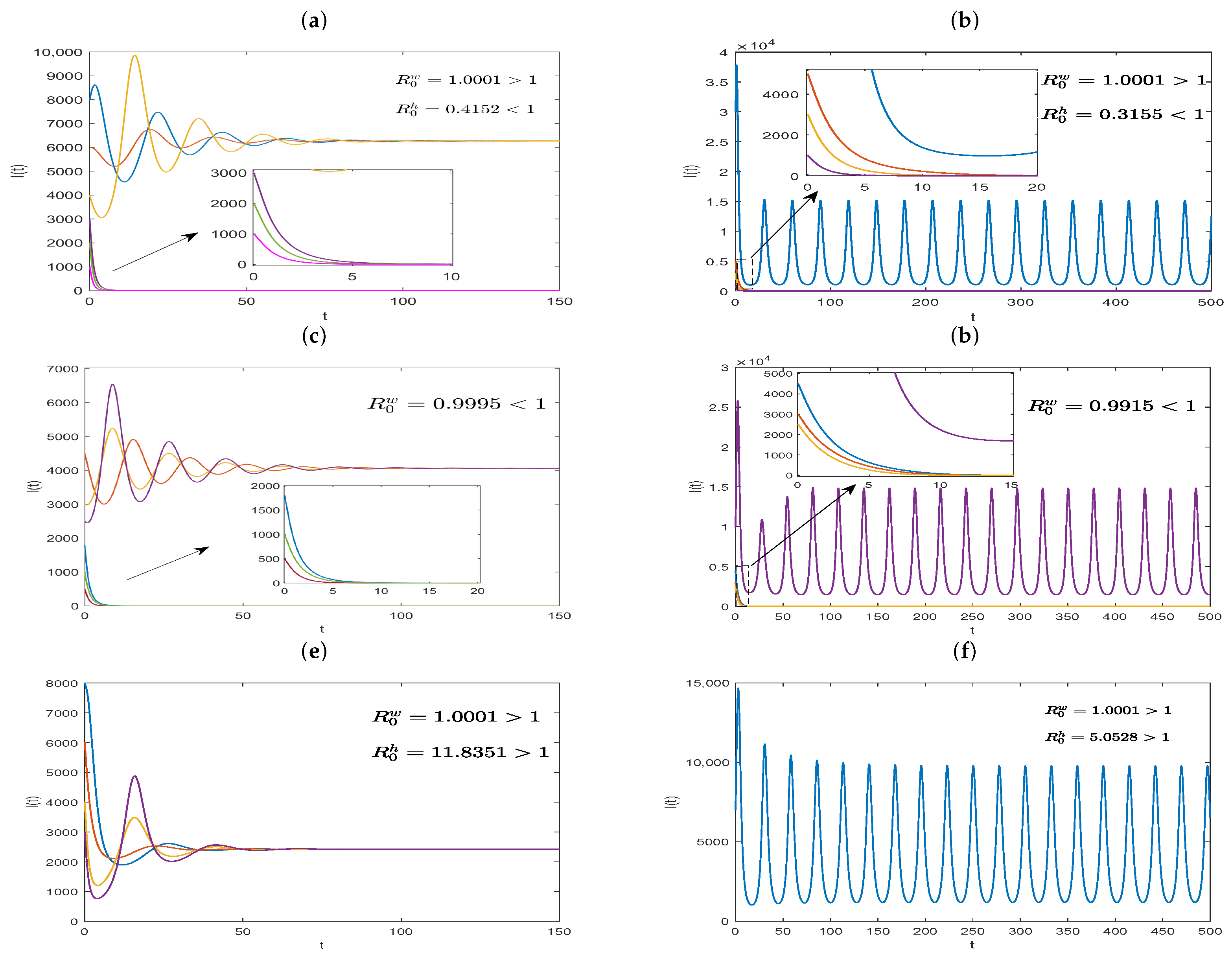
Author Contributions

Conceptualization, M.W. and L.N.; methodology, M.W., Y.W., L.H. and L.N.; software, M.W.; validation, M.W., Y.W., L.H. and L.N.; formal analysis, M.W. and L.N.; writing—original draft preparation, M.W.; writing—review and editing M.W. and L.N. All authors have read and agreed to the published version of the manuscript.

Funding

This research was funded by the Natural Science Foundation of Xinjiang Uygur Autonomous Region (Grant Nos. 2022TSYCCX0015 and 2021D01E12), the National Natural Science Foundation of China (Grant No. 12361103).

Institutional Review Board Statement

Not applicable.

Informed Consent Statement

Not applicable.

Data Availability Statement

No new data were created or analyzed in this study. Data sharing is not applicable to this article.

Acknowledgments

The authors are thankful to the anonymous reviewers for their careful reading, useful comments, and constructive suggestions for the improvement of the present research work. We are also thankful to the editor for his speed and cooperation.

Conflicts of Interest

The authors declare no conflicts of interest.

References

  1. Westem, K.A. National Institute of Allergy and Infectious Disease. Reseach Conf. Natl. Inst. Allergy Infect. Dis. 2008, 1, 3–8. [Google Scholar]
  2. Whiteside, A. HIV and AIDS: A Very Short Introduction; Oxford University Press: Oxford, UK, 2016. [Google Scholar]
  3. HIV Statistic Globally and by WHO Region, 2023. Available online: https://www.who.int/teams/global-hiv-hepatitis-and-stis-programmes/hiv/strategic-information/hiv-data-and-statistics (accessed on 18 July 2023).
  4. Mccluskey, C.C. A model of HIV/AIDS with staged progression and amelioration. Math. Biosci. 2003, 181, 1–16. [Google Scholar] [CrossRef]
  5. Samanta, G.P. Permanence and extinction of a nonautonomous HIV/AIDS epidemic model with distributed time delay. Nonlinear Anal. Real 2011, 12, 1163–1177. [Google Scholar] [CrossRef]
  6. Perelson, A.S.; Neumann, A.U.; Markowitz, M.; Leonard, J.M.; Ho, D.D. HIV-1 dynamics in vivo: Virion clearance rate, infected cell life-span, and viral generation time. Science 1996, 271, 1582–1586. [Google Scholar] [CrossRef]
  7. Zhu, H.Y.; Zou, X.F. Dynamics of a HIV-1 infection model with cell-mediated immune response and intracellular delay. Discrete Cont. Dyn. B 2009, 12, 511–524. [Google Scholar] [CrossRef]
  8. Virgin, H.W.; Walker, B.D. Immunology and the elusive AIDS vaccine. Nature 2010, 464, 224–231. [Google Scholar] [CrossRef]
  9. Roederer, M.; Keele, B.F.; Schmidt, S.D.; Mason, R.D.; Welles, H.C.; Fischer, W.; Labranche, C. Immunological and virological mechanisms of vaccine-mediated protection against SIV and HIV. Nature 2014, 505, 502–508. [Google Scholar] [CrossRef]
  10. Wang, S.; Zou, D. Global stability of in-host viral models with humoral immunity and intracellular delays. Appl. Math. Model. 2012, 36, 1313–1322. [Google Scholar] [CrossRef]
  11. Murase, A.; Sasaki, T.; Kajiwara, T. Stability analysis of pathogen-immune interaction dynamics. J. Math. Biol. 2005, 51, 247–267. [Google Scholar] [CrossRef]
  12. Huang, G.; Takeuchi, Y.; Ma, W.; Wei, D. Global stability for delay SIR and SEIR epidemic models with nonlinear incidence rate. B. Math. Biol. 2010, 72, 1192. [Google Scholar] [CrossRef]
  13. Xu, R. Global dynamics of an SEIS epidemiological model with time delay describing a latent period. Math. Comput. Simulat. 2012, 785, 90–102. [Google Scholar] [CrossRef]
  14. Farah, E.M.; Amine, S.; Allali, K. Dynamics of a time-delayed two-strain epidemic model with general incidence rates. Chaos Soliton. Fract. 2021, 153, 111527. [Google Scholar] [CrossRef]
  15. Tipsri, S.; Chinviriyasit, W. The effect of time delay on the dynamics of an SEIR model with nonlinear incidence. Chaos Soliton. Fract. 2015, 75, 153–172. [Google Scholar] [CrossRef]
  16. Jiang, Z.; Ma, W.; Wei, J. Global hopf bifurcation and permanence of a delayed SEIRS epidemic model. Math. Comput. Simulat. 2016, 122, 35–54. [Google Scholar] [CrossRef]
  17. Culshaw, R.V.; Ruan, S.; Webb, G. A mathematical model of cell-to-cell spread of HIV-1 that includes a time delay. J. Math. Biol. 2003, 46, 425–444. [Google Scholar] [CrossRef]
  18. Xu, R. Global stability of an HIV-1 infection model with saturation infection and intracellular delay. Comput. Math. Appl. 2011, 61, 2799–2805. [Google Scholar] [CrossRef]
  19. Liu, H.; Zhang, J.F. Dynamics of two time delays differential equation model to HIV latent infection. Phys. A 2019, 541, 384–395. [Google Scholar] [CrossRef]
  20. Pawelek, K.A.; Liu, S.; Pahlevani, I.F.; Rong, L.B. A model of HIV-1 infection with two time delays: Mathematical analysis and comparison with patient data. Math. Biosci. 2012, 235, 98–105. [Google Scholar] [CrossRef]
  21. Lin, J.; Xu, R.; Tian, X. Threshold dynamics of an HIV-1 virus model with both virus-to-cell and cell-to-cell transmissions, tntracellular delay, and humoral immunity. Appl. Math. Comput. 2017, 315, 516–530. [Google Scholar]
  22. Yang, Y.; Huang, G.; Dong, Y.P. Stability and Hopf bifurcation of an HIV infection model with two time delays. Math. Biosci. Eng. 2023, 20, 1938–1959. [Google Scholar] [CrossRef]
  23. Feng, Z.L.; Velasco-Hernandez, J.; Tapia-Santos, B.; Leite, M.C.A. A model for coupling within-host and between-host dynamics in an infectious disease. Nonlinear Dynam. 2011, 68, 401–411. [Google Scholar] [CrossRef]
  24. Lingappa, J.R.; Hughes, J.P.; Wang, R.S.; Baeten, J.M.; Connie, C.; Gray, G.E.; Stevens, W.S.; Deborah, D.; Campbell, M.S.; Carey, F. Estimating the impact of plasma HIV-1 RNA reductions on heterosexual HIV-1 transmission risk. PLoS ONE 2010, 5, e12598. [Google Scholar] [CrossRef] [PubMed]
  25. Cohen, M.; Chen, Y.Q.; Mccauley, M.; Fleming, T.R. Prevention of HIV-1 infection with early antiretroviral therapy. New Engl. J. Med. 2011, 365, 493–505. [Google Scholar] [CrossRef] [PubMed]
  26. Gilchrist, M.A.; Sasaki, A. Modeling host-parasite coevolution: A nested spproach based on mechanistic models. J. Theor. Biol. 2002, 218, 289–308. [Google Scholar] [CrossRef] [PubMed]
  27. Gilchrist, M.A.; Coombs, D. Evolution of virulence: Interdependence, constraints, and selection using nested models. Theor. Popul. Biol. 2006, 69, 145–153. [Google Scholar] [CrossRef] [PubMed]
  28. Boldin, B.; Diekmann, O. Superinfections can induce evolutionarily stable coexistence of pathogens. J. Math. Biol. 2008, 56, 635–672. [Google Scholar] [CrossRef] [PubMed]
  29. Feng, Z.L.; Velasco-Hernandez, J.; Tapia-Santos, B. A mathematical model for coupling within-host and between-host dynamics in an environmentally infectious disease. Math. Biosci. 2013, 241, 49–55. [Google Scholar] [CrossRef] [PubMed]
  30. Cen, X.L.; Feng, Z.L.; Zhao, Y.L. Emerging disease dynamics in a model coupling within-host and between-host systems. J. Theor. Biol. 2014, 361, 141–151. [Google Scholar] [CrossRef]
  31. Feng, Z.L.; Cen, X.L.; Zhao, Y.L.; Velasco-Hernandez, J. Coupled within-host and between-host dynamics and evolution of virulence. Math. Biosci. 2015, 270, 204–212. [Google Scholar] [CrossRef]
  32. Wang, X.Y.; Wang, S.P.; Wang, J.; Rong, L.B. A multiscale model of COVID-19 dynamics. Bull. Math. Biol. 2022, 84, 99. [Google Scholar] [CrossRef]
  33. Xue, Y.Y.; Xiao, Y.N. Analysis of a multiscale HIV-1 model coupling within-host viral dynamics and between-host transmission dynamics. Math. Biosci. Eng. 2020, 17, 6720–6736. [Google Scholar] [CrossRef]
  34. Wang, J.L.; Zou, X.F.; Lang, J.Y. Analysis of an age structured HIV infection model with virus-to-cell infection and cell-to-cell transmission. Nonlinear Anal.-Real 2017, 34, 75–96. [Google Scholar] [CrossRef]
  35. Hale, J.K.; Lunel, S.M.V. Introduction to Functional Differential Equations; Springer: New York, NY, USA, 1993. [Google Scholar]
  36. Li, X.L.; Wei, J.J. On the zeros of a fourth degree exponential polynomial with applications to a neural network model with delays. Chaos Solitons Fractals 2005, 26, 519–526. [Google Scholar] [CrossRef]
  37. Hale, J.K. Theory of Functional Differential Equations; Springer: New York, NY, USA, 1977. [Google Scholar]
  38. Liang, X.; Zhao, X.Q. Asymptotic speeds of spread and traveling waves for monotone semiflows with applications. Commun. Pur. Appl. Math. 2007, 60, 1–40. [Google Scholar] [CrossRef]
  39. Hassard, B.D.; Kazarinoff, N.D.; Wan, Y.H. Theory and Applications of Hopf Bifurcation; Cambridge University Press: Cambridge, UK, 1981. [Google Scholar]
  40. Song, Y.L.; Wei, J.J. Bifurcation analysis for Chen’s system with delayed feedback and its application to control of chaos. Chaos Solitons Fractals 2004, 22, 75–91. [Google Scholar] [CrossRef]
  41. Zhao, X.Q. Basic reproduction ratios for periodic compartmental models with time delay. J. Dyn. Differ. Equ. 2017, 29, 67–82. [Google Scholar] [CrossRef]
  42. Smith, H.L. Monotone Dynamical Systems: An Introduction To the Theory of Competitive and Cooperative Systems; American Mathematical Society: Providence, RI, USA, 1995. [Google Scholar]
  43. Zhao, X.Q. Dynamical Systems in Population Biology; Springer: Cham, Switzerland, 2003. [Google Scholar]
  44. Wang, X.; Zhao, X.Q. A periodic vector-bias malaria model with incubation period. SIAM. J. Appl. Math. 2017, 77, 181–201. [Google Scholar] [CrossRef]
  45. Wang, X.; Zhao, X.Q. Dynamics of a time-delayed Lyme disease model with seasonality. SIAM. J. Appl. Dyn. Syst. 2017, 16, 853–881. [Google Scholar] [CrossRef]
  46. Hale, J.K. Asymptotic Behavior of Dissipative Systems; American Mathematical Society: Providence, RI, USA, 1988. [Google Scholar]
  47. Nowak, M.A.; Bangham, C.R. Population dynamics of immune responses to persistent viruses. Science 1996, 272, 74–79. [Google Scholar] [CrossRef]
  48. Yang, T.H.; Zhang, L. Remarks on basic reproduction ratios for periodic abstract functional differential equations. Discrete Cont. Dyn. B 2019, 24, 6771–6782. [Google Scholar] [CrossRef]
  49. World Health Organization. Available online: https://www.who.int/director-general/speeches/detail/who-director-general-s-opening-remarks-at-the-media-briefing---26-july-2023 (accessed on 26 July 2023).
Figure 1. A flowchart for the multiscale Model (1) and Model (2).
Axioms 13 00147 g001
Figure 2. The existence and stability of the immunity-inactivated infection equilibrium, U ˜ 1 , of Model (4) when R w = 0.4812 < 1 : (a) the existence of U ˜ 1 ; (b) the stability of U ˜ 1 .
Axioms 13 00147 g002
Figure 3. Dynamics of the full system with different cases, where the different colored lines represent the trajectories of I ( t ) with different initial values: (a) R 0 w = 1.0001 > 1 and R 0 h = 0.4152 < 1 , where I ( t ) may tend to zero or to a constant value, which depends on the state of the infected individuals at the initial moment; (b) R 0 w = 1.0001 > 1 and R 0 h = 0.3155 < 1 , where I ( t ) may tend to zero or may show cyclic oscillatory behavior and the model admits a Hopf bifurcation; (c) R 0 w = 0.9995 < 1 , which is similar to (a); (d) R 0 w = 0.9915 < 1 , which is similar to (b); (e) R 0 h = 11.8351 > 1 and R 0 w = 1.0001 > 1 , the existence and global asymptotic stability of the endemic equilibrium; (f) R 0 h = 5.0528 > 1 and R 0 w = 1.0001 > 1 , the existence of a positive periodic solution, which implies delay induces the Hopf bifurcation.
Axioms 13 00147 g003
Figure 4. Illustration of the bifurcation diagrams, where I ˜ is a function of R 0 h and R 0 w , with the black solid curve, red solid curve, and blue dashed curve representing the locally asymptotically stable, conditionally stable, and unstable equilibrium, respectively. (a) When R 0 w > 1 , changing R 0 h , the saddle-node bifurcation occurs at R h c = 0.252 . For R 0 h ( R h c , 1 ) , there are two positive equilibria, where one is conditionally stable and the other is unstable; for R 0 h > 1 , there is a unique conditionally stable positive equilibrium. (b) Changing R 0 w , the saddle-node bifurcation occurs at R w c = 0.99838 . The existence and stability of the positive equilibrium for R 0 w ( R w c , 1 ) is the same as that of the situation R 0 h ( R h c , 1 ) .
Axioms 13 00147 g004
Figure 5. The existence and stability of immunity-activated infection equilibrium, U ˜ 2 , of the fast time model (4) when R w = 19.0010 > 1 : (a) the existence of U ˜ 2 ; (b) the stability of U ˜ 2 .
Axioms 13 00147 g005
Figure 6. The dynamics of the coupled slow time model (28) with an immune response: (a,b) the existence and stability of E ˜ 0 when R ˜ 0 h = 0.3103 < 1 ; (c,d) the existence and stability of E * when R ˜ 0 h = 10.7084 > 1 .
Axioms 13 00147 g006
Figure 7. The dynamics of the fast time model (4) with τ 2 = 3.4 > τ 2 * = 3.22 and τ 1 = 0.8 , where the infection equilibrium, U ˜ 2 , is unstable and the model (4) exists in a stable periodic solution: (a) the time series charts of T ( s ) , T * ( s ) , V ( s ) and B ( s ) ; (b) three-dimensional phase diagram of ( T , T * , V ) ; (c,d) the stability of the periodic solution.
Axioms 13 00147 g007
Figure 8. Periodic solution fitting: (a) the time series of V ( s ) of the fast time model (4); (b) the function fitting of periodic solution V ˜ ( s ) , where the curve formed by the black dot represents the time series of V ˜ ( s ) , and the red represents the fitting curve.
Axioms 13 00147 g008
Figure 9. Long-term behaviors of Model (34), where the blue, red and black lines represent the trajectories of S ( t ) , I ( t ) and A ( t ) , respectively. (a,b) The existence and stability of the disease-free periodic solution E 0 ( t ) when R 0 < 1 . (c,d) The existence of the positive periodic solution E ¯ ( t ) when R 0 > 1 .
Axioms 13 00147 g009
Figure 10. The influence of main parameters on the infected individuals I ( t ) and A ( t ) for Model (33) when R 0 > 1 : (a,b) the effect of the latency period τ ; (c,d) the effect of contact rate c 1 ; (e,f) the effect of contact rate c 2 .
Axioms 13 00147 g010
Table 1. The biological interpretations of parameters in Model (1).
ParameterThe Biological Meanings
Λ h Total birth/recruitment rate of hosts
c 1 , c 2 The mean number of contacts with individuals who are HIV-positive and those with
AIDS, respectively
β 1 ( V ) , β 2 ( V ) Transmission rates of HIV-positive individuals and AIDS patients, respectively
μ Natural mortality of hosts
τ Latent period of virus in vivo
e μ τ The surviving rate of infected individuals during latent period τ
ξ Transfer rate from HIV-positive stage to the AIDS patients stage
δ 1 ( V ) , δ 2 ( V ) Disease-induced mortality of HIV-positive individuals and AIDS patients, respectively
Table 2. The biological interpretations of parameters in Model (2).
ParameterThe Biological Meanings
Λ c Recruitment rates of healthy cells
κ 1 , κ 2 Infection rates of virus-to-cell transmission and cell-to-cell transmission, respectively
μ c Natural mortality rate of cells (healthy cells and infected cells)
τ 1 Intracellular delay (see [21] for more detail)
e μ c τ 1 The probability of surviving the time period from s τ 1 to s
δ c Disease-induced mortality of infected cells
η 1 , η 2 The quantity of virus that HIV-positive individuals and AIDS patients release
during each contact
pThe quantity of viral particles generated by each infected cell
qThe number of viral particles killed by each B cell
μ v Virus clearance rate within the host
σ Production rate of new B cells stimulated by antigen
τ 2 The time required for antigenic stimulation to generate B cells
ζ Death rate of B cells
Disclaimer/Publisher’s Note: The statements, opinions and data contained in all publications are solely those of the individual author(s) and contributor(s) and not of MDPI and/or the editor(s). MDPI and/or the editor(s) disclaim responsibility for any injury to people or property resulting from any ideas, methods, instructions or products referred to in the content.