Computing Transiting Exoplanet Parameters with 1D Convolutional Neural Networks

Abstract

The transit method allows the detection and characterization of planetary systems by analyzing stellar light curves. Convolutional neural networks appear to offer a viable solution for automating these analyses. In this research, two 1D convolutional neural network models, which work with simulated light curves in which transit-like signals were injected, are presented. One model operates on complete light curves and estimates the orbital period, and the other one operates on phase-folded light curves and estimates the semimajor axis of the orbit and the square of the planet-to-star radius ratio. Both models were tested on real data from TESS light curves with confirmed planets to ensure that they are able to work with real data. The results obtained show that 1D CNNs are able to characterize transiting exoplanets from their host star’s detrended light curve and, furthermore, reducing both the required time and computational costs compared with the current detection and characterization algorithms.

1. Introduction

Exoplanet detection is one of the most relevant fields in astrophysics nowadays. Its origins trace back to 1992, when the discovery of three exoplanets orbiting the $PSR1257+12$ pulsar [1] emerged from data collected by the 305 m Arecibo radio telescope. This discovery was the beginning of a new research area that is still being studied nowadays, although this planetary system is not what they were looking for, as the surroundings of a pulsar are completely different from the one surrounding a star in which there could be planets similar to the Earth.

Over the years, various detection techniques have been established. One of the most used is the transit method, which consists of detecting periodic dimmings in the stellar light curves (which are the flux in the function of the time) due to the crossing of an exoplanet (or more) with the line of sight between its host star and a telescope monitoring it. This is probably the most used technique nowadays, as there are a lot of photometry data available from different surveys, as one telescope can monitor thousands of stars at the same time. The first discovery of exoplanets related to this technique took place in the year 2000, when [2,3] discovered an exoplanet orbiting the star HD 209458. The dimmings detected through this technique are described by the Mandel and Agol theoretical shape [4], which takes into account an optical effect known as limb darkening, which makes the star appear less bright at the edges than at the center. From these models, it is possible to estimate the orbital period (P), which is the temporal distance between two consecutive transits; the planet-to-star radius ratio ($R_p/R_{★}\equiv R_p\left[R_{★}\right]$), which is related to the transit depth; the semimajor axis of the orbit in terms of the stellar radius ($a/R_{★}\equiv a\left[R_{★}\right]$); and the orbital plane inclination angle (i).

The main challenges related to the analysis of light curves when trying to search and characterize transit-like signals are the high computational cost required to analyze the large dataset of light curves available from different surveys, the high amount of time required to visually inspect them; and the fact that stellar noise present in light curves could make the transit detection considerably more difficult.

One of the most relevant solutions to these problems comes from artificial intelligence (AI). If an AI model could be able to distinguish between transit-like signals and noise, it would reduce the amount of light curves that are needed to analyze with current algorithms.

Current algorithms, such as box least squares (BLS) [5] and transit least squares (TLS) [6], among others, could be classified mainly into Markov chain Monte Carlo (MCMC) methods and least squares algorithms. The second ones, including BLS and TLS, search for periodic transit-like signals in the light curves and compute some of the most relevant parameters related to the transit method (as P, $R_p\left[R_{★}\right]$, etc.). However, BLS needs about 3 s per light curve and TLS about 10 s (taking into account the simulated light curves explained in Section 2.2 and the server used in this research (see Section 3)), making the analysis of thousands of light curves within a short timeframe exceedingly challenging.

The TESS (Transiting Exoplanet Survey Satellite) mission [7] is a space telescope launched in April 2018, whose main goal is to discover exoplanets smaller than Neptune through the transit method, orbiting stars bright enough to be able to estimate their companions’ atmospheres. The telescope is composed of 4 cameras with 7 lenses, thus allowing for monitoring a region of ${24}^{\circ }\times {96}^{\circ }$ during a sector (27 days). It took data with long and short cadence (30 min and 2 min, respectively). Its prime mission started in July 2018 and finished in April 2020. Currently, it is developing an extended mission, which started in May 2020. It is important to remark that TESS light curves obtained from full frame images (FFIs) usually present high noise levels in less bright stars, which makes planetary detection and characterization considerably more difficult.

Understanding exoplanet demographics in the function of the main stellar parameters is important not only for checking and improving planetary evolution and formation models, but also for studying planetary habitability [8]. The main parameters on which to calculate demographics can be split into three main groups: planetary system, host star, and surrounding environment. First of all, it is important to remark that all detection techniques have clear bias related to which type of planets are able to detect, which greatly conditions the study of planetary demography. One example is the radial velocity (RV) technique, which consists of measure Doppler shifts in stellar spectra due to the gravitational interaction between the planets and their host star, which is highly dependent on the planet-to-star mass ratio. From [9,10], it was estimated that ∼20% of solar-type stars host a giant exoplanet (i.e., $M_P>0.3M_J$, where $M_J$ is the Jupiter mass) at 20 AU. The main contributions of RV research to planet demographics ([11,12] among others) include that, in solar-type stars and considering a short orbital period regime, low mass planets are up to an order of magnitude more probable than giant ones. In addition, the giant planet occurrence rate increases along with the period up to about 3 AU from its host star, and also, if they are closer to 2.5 AU, these rates increase with stellar mass and metallicity ($[Fe/H]$). Finally, Neptune-like planets are the most frequent beyond the frost line [13] (the minimum distance from the central protostar in a solar nebula, where the temperature drops sufficiently to allow the presence of volatile compounds like water). Other techniques, such as transits, also help to study planetary demographics. It is necessary to highlight the contributions of the Kepler [14] mission. Its exoplanet data allowed the study of the bimodality in the small planet size’s distribution [15] and the discovery of the Neptune dessert [16], which is a term used to describe the zone near a star ($P<2-4d$) where the absence of Neptune-sized exoplanets is observed. In addition, as most of the stars appear to host a super-Earth (or sub-Neptune), which is a type of planet that is not present in the Solar System, it seems that our planetary system architecture might not be much common. All the transit-based detection facilities in general and TESS in particular show clear bias in the planetary systems found. Statistics from [17] show that it is more common to find planetary systems with low orbital period, as this produces a greater number of transits in the light curves. Additionally, planets with low planet-to-star radius ratio and semimajor axis are more frequent.

Machine learning (ML) techniques allow for setting aside human judgment in order to detect and fit transit-like signals in light curves, thus reducing the overall time and computational cost required to analyze all of them. The first approach was the Robovetter project [18], which was used to create the seventh Kepler planet candidate (PC) catalog, employing a decision tree for classifying threshold crossing events (TCEs), which are periodic transit-like signals. Others, such as Signal Detection using Random forest Algorithm (SIDRA) [19], used random forests in order to classify TCEs depending on different features related to transit-like signals. Artificial neural networks (ANNs) were thought to be a better solution, in particular convolutional neural networks (CNNs). The results from [20,21,22,23,24,25,26,27,28] show that CNNs perform better in transit-like signal detection due to the fact that these algorithms are prepared for pattern recognition. One example was carried out in our previous work [28], in which the performance of 1D CNN in transit detection was shown by training a model on K2 simulated data. Nowadays, as current and future observing facilities provide very large datasets composed of many thousands of targets, automatic methods, such as CNN, are crucial for analyzing all of them.

In this research, we continue to go a step further. As our previous results showed, 1D CNNs are able to detect the presence of transit-like signals in light curves. The aim of this research is to develop 1D CNN models that are able to extract different planetary parameters from light curves in which it is known that there are transit-like signals. There are other techniques that allow being automatized with ML techniques. One example was carried out in [29], which studied how deep learning techniques can estimate the planetary mass from RV data.

Our models were trained with simulated light curves that mimic those expected for the TESS mission, as there are not enough confirmed planets detected with TESS (with their respective host star’s light curves) to train a CNN model. The reasons why simulated TESS light curves were used instead of K2 ones are motivated by the fact that apart from checking the performance of CNN in transit-like signal characterization, another aim is to check their performance with light curves from another survey. Our light curve simulator was adapted for creating both complete and phase-folded light curves. This comes from the fact that for phase-folding a light curve, first, it is necessary to know the orbital period of the planet (which is computed as the distance between two consecutive transits). After knowing this parameter, a phase-folded light curve could be computed by folding the complete light curve in the function of the orbital period. This is crucial because, taking into account the most common observing cadence from the main telescopes (about 30 min), a transit with a duration of a few hours could be represented with only a few points, which makes the transit model fitting considerably difficult. By phase-folding a light curve, the transit shape is much more precise, as it is composed of all the in-transit data points from the complete light curve. From the complete light curves, our model is able to compute the orbital period, and from the phase-folded light curve, it calculates the planet-to-star radius ratio and the semimajor axis in terms of its host star radius (see Section 3).

The rest of this paper is structured as follows: In Section 2, the materials and methods used during the research are explained. More concretely, in Section 2.1, the theoretical transit shape, which appears in all the light curves with which our models are trained, is explained; in Section 2.2, light curve simulation is detailed; and in Section 2.3, the structure of our model is shown in detail. In Section 3, the training, test, and validation processes of the model are explained, and also the statistics related to the predicted values obtained during the test process and the model test on real TESS data are shown and discussed. Finally, in Section 4, the conclusions of all the research are outlined.

2. Materials and Methods

In this section, the main materials and methods used during this research are introduced, including the explanation of the transit theoretical shape, the light curve simulation, and CNNs, placing special emphasis on the models used.

2.1. Transit Shape

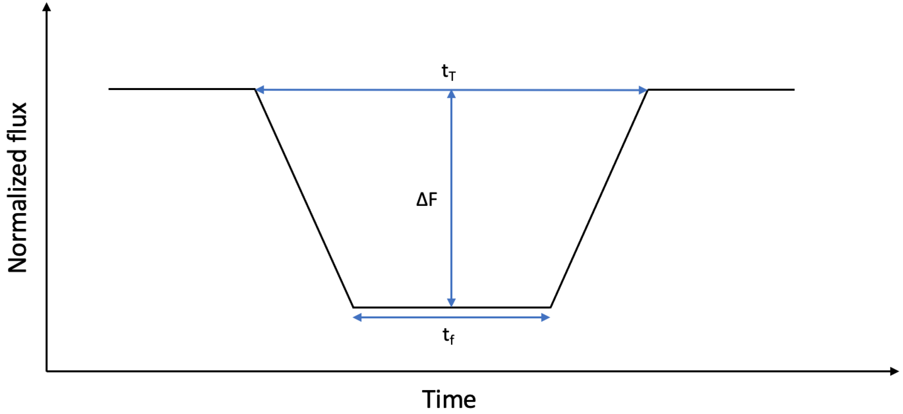
Theoretically, a transit can be described as a trapezoid where the amount of flux that reaches the detector decreases while the planet overlaps the star. There are 3 main parameters that can be derived from its shape: the transit depth ($\Delta F$), the transit duration ($t_T$), and the duration of the flat region ($t_F$), which is observed when the whole planet is overlapping the star (see Figure 1).

The flux that arrives at the detector, which is monitoring the star, could be expressed as [4]

$$F(a\left[r_{★}\right],R_p\left[R_{★}\right])=1-\lambda (a\left[r_{★}\right],R_p\left[R_{★}\right]),$$

(1)

where $F(a\left[r_{★}\right],R_p\left[R_{★}\right])$ is the flux that reaches the telescope and $\lambda (a\left[r_{★}\right],R_p\left[R_{★}\right])$ is the portion of the flux that is blocked by the planet. As the planet overlaps the star, the amount of flux decreases.

Actually, the transit shape is more complex as there is an optical effect that makes the star appear less bright at the edges than at the center, known as limb darkening. This effect causes the transit to be rounded. The most accurate transit shape, taking into account this phenomenon, is described in [4] (Mandel and Agol theoretical shape). The limb darkening formulation adopted in the Mandel and Agol shape is described in [30], where how the intensity emitted by the star changes in the function of the place where the radiation comes from is described:

$$\frac{I\left(\mu \right)}{I\left(0\right)}=1-\sum _{m=1}^4{c}_m(1-{\mu }^{m/2}),$$

(2)

with $\mu =\sqrt{1-{\tilde{r}}^2}$, where $\tilde{r}\in [0,1]$ is the normalized radial coordinate on the disk of the star, $c_m$ are the limb darkening coefficients, and I(0) is the intensity at the center of the star. Another common parameterization of this phenomenon is made with a quadratic law [31], where $u_1$ and $u_2$ are the quadratic limb darkening coefficients:

$$\frac{I\left(\mu \right)}{I\left(0\right)}=1-u_1·(1-\mu )-u_2·{(1-\mu )}^2.$$

(3)

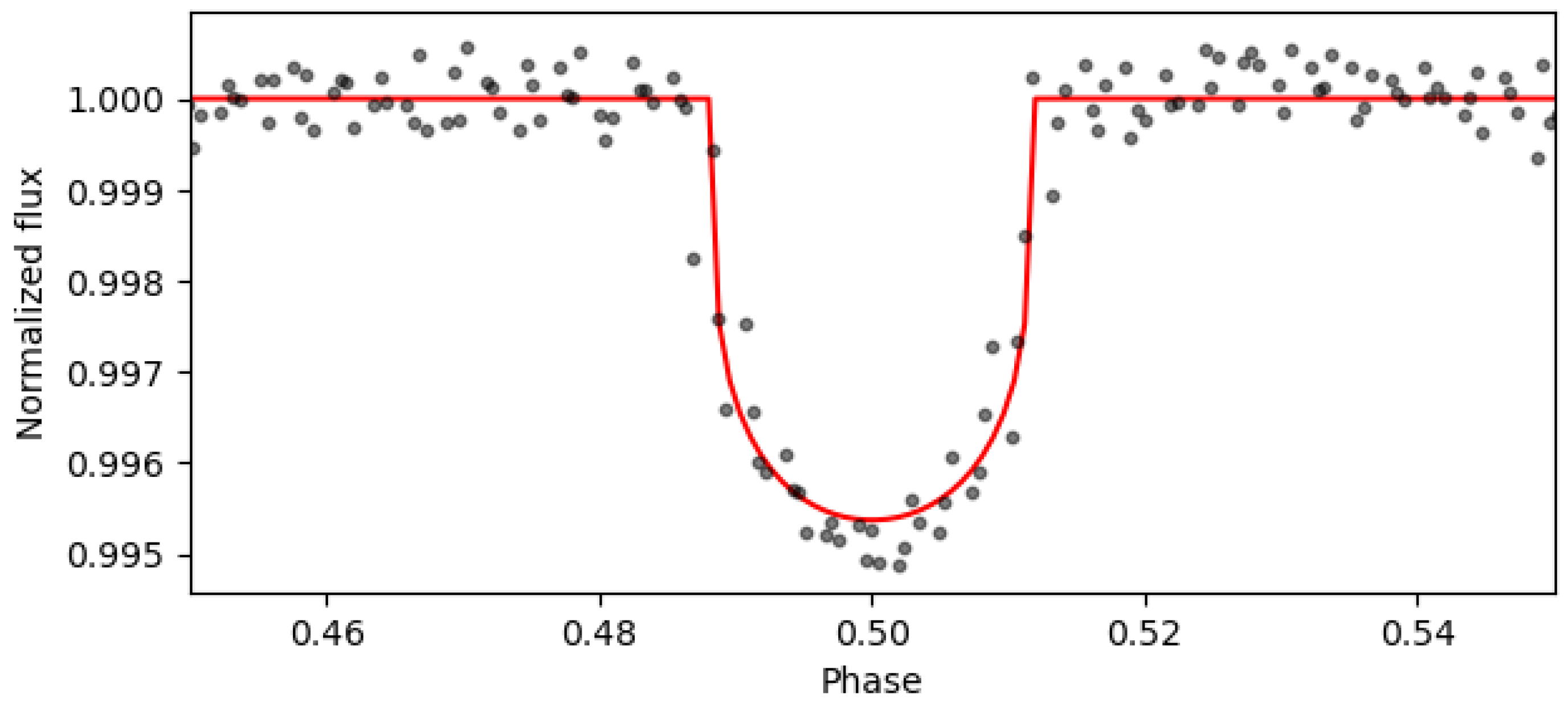
Taking into account the limb darkening effect, the Mandel and Agol theoretical shape models transits as

$$F(a\left[r_{★}\right],R_p\left[R_{★}\right])={\left[{\int }_0^{1}dr2rI\left(r\right)\right]}^{-1}{\int }_0^{1}drI\left(r\right)\frac{d\left[\tilde{F}(a\left[r_{★}\right]/r,R_p\left[R_{★}\right]/r]\right)}{dr},$$

(4)

where $\tilde{F}(a\left[r_{★}\right]/r,R_p\left[R_{★}\right]/r])$ is the transit shape without the limb darkening effect. An example of the Mandel and Agol transit shape obtained with TLS from a simulated light curve (see Section 2.2) is shown in Figure 2. The value $t_f$ is much more difficult to determine. However, as was previously mentioned, it is still possible to estimate different parameters, as in the case of $R_p\left[R_{★}\right]$, which is related to the squared root of the mean depth of the transit. For this reason, it is thought that convolutional neural networks, which learn from the input dataset shape, could be a solution. They could infer the main parameters from a phase-folded light curve. Others, as the orbital period, should be inferred from the complete light curve, because its value is the mean distance between two consecutive transits.

2.2. Light Curve Simulation

The aim of this research is the creation of a CNN architecture that is able to predict the values P, $R_p\left[R_{★}\right]$, and $a\left[R_{★}\right]$ and that is trained with TESS light curves. However, as a CNN needs a large dataset for training all its hyperparameters, and there are not enough real light curves with confirmed planetary transits to train it, it was decided to use simulated light curves to train and test the models. This is why the light curve simulator used in our previous work was adapted to TESS data. It is important to remark that TESS light curves are shorter than K2 ones due to the fact that TESS observes a sector during 27 days instead of 75 days (which is the mean duration of K2 campaigns). In contrast, as both of them have a mean observing cadence of 30 min, the observing cadence was not changed. However, less bright stars were selected in order to increase the noise levels, which would mean that the network would also be able to learn to characterize transits where noise levels make this work considerably much more difficult.

Before explaining our light curve simulator, it is necessary to clarify that stellar light curves are affected by stellar variability phenomena, such as rotations, flares, and pulsations, which induce trends that have to be removed before analyzing them. The light curves after removing these trends are usually known as detrended (or normalized) light curves.

For simulating light curves, the Batman package [32], which allows for creating theoretical normalized light curves with transits (i.e., detrended light curves with transits but without noise), was used. The main parameters needed for creating the transit models are the orbital period (P); the planet-to-star radius ratio ($R_p\left[R_{★}\right]$); the semimajor axis in terms of the host star’s radius ($a\left[r_{★}\right]$); the epoch ($t_0$), which is the time in which the first transit takes place; the inclination angle of the orbital plane ($i\left[deg\right]$); and the limb darkening quadratic coefficients ($u_1$ and $u_2$).

All these parameters were selected, when it was possible, as random values, where the upper and lower limits were chosen, taking into account planetary statistics (in general, not only the TESS ones) or the main characteristics of TESS light curves. As previously mentioned, as the TESS mission detects exoplanets through the transit method, it is more common to find planetary systems with low periods, planet-to-star radius ratio, and semimajor axis. However, as the main objective is to develop a model that is as most generalized as possible, it was decided not to use these statistics, thus preventing the model from generating dependence and not being able to correctly characterize systems with different parameters. First of all, it was decided to inject at least 2 transits in the light curves (necessary to be able to estimate the orbital period from light curves), so the maximum value of the period considered is half of the duration of the light curves. The value is chosen randomly between these limits. This is the only restriction applied that generates bias in the data, but it is necessary to apply it because if there were not at least 2 transits in the light curves, the model would not be able to estimate the orbital period. Then, the epoch was chosen as a random value between 0 and the value of the orbital period.

For choosing $R_p\left[R_{★}\right]$, the following procedure was carried out: First of all, it is necessary to simulate the host star. The stellar mass was chosen as a random value following the statistics of the solar neighborhood, which is the surrounding region to the Sun within ∼92 pc. Their radii were estimated following the mass–radius relationship of the main sequence (MS) stars [33,34] (among others):

$$R_{★}\left[R_{\odot }\right]\sim {\left(M_{★}\left[M_{\odot }\right]\right)}^{0.8}$$

(5)

The distance and apparent magnitude (which is a measure of the brightness of a star observed from the Earth on an inverse logarithmic scale) were chosen as random values limited, respectively, by the solar neighborhood size (up to ∼92 pc) and TESS typically detected magnitudes (up to magnitude 16) [7]. Limb darkening quadratic parameters ($u_1$ and $u_2$) are chosen as random values between 0 and 1 considering $u_1+u_2=1$. Then, the planetary radius was chosen following planetary statistics: it is not common to find Jupiter-like exoplanets orbiting low mass stars as red dwarfs, so the maximum radius of the orbiting exoplanet was limited to the one expected from a Neptune-like one in low mass stars (i.e., the maximum $R_p\left[R_{★}\right]$ was set to $0.05$ for stars with masses lower than $0.75M_{\odot }$). For more massive stars, the upper limit is a Jupiter-like exoplanet (i.e., the maximum value is limited to $R_p\left[R_{★}\right]=0.1$ if the stellar mass is larger than $0.75M_{\odot }$). $a\left[r_{★}\right]$ was derived considering Kepler’s third law:

$$a={\left(\frac{G·M_{★}}{4·{\pi }^2}·P^2\right)}^{\frac{1}{3}}.$$

(6)

To summarize all the stellar and planetary parameters used during the light curve simulation, the upper and lower limits from all of them are shown in

Table 1. Stellar and planetary paramaters’ upper and lower limits used for simulating the light curves.

Parameter	Min Value	Max Value
$M_{★}\left[M_{\odot }\right]$	0.1	10
$R_{★}\left[R_{\odot }\right]$	0.15	4.89
$u_1$	0	1
$u_2$	0	1
mag	8	16
$d\left[pc\right]$	1	92
$P\left(d\right)$	1	13.5
$t_0$	0	$P\left(d\right)$
$R_p\left[R_{★}\right]$	0.01	0.1

.

As was already mentioned, phase-folded light curves, which allowed for obtaining more accurate transit shapes, thus producing better performance in transit characterization, were also simulated. The main difference when creating both types of light curves is that in the complete light curve, the temporal vector needed for simulating them takes into account the whole duration of a TESS sector; on the contrary, a phase-folded light curve is created with a temporal vector between $t_0-P/2$ and $t_0+P/2$, which other authors call as a global view of the transit (a local version will be created by making a zoom to the transit) [22,24] (among others).

Batman creates light curves without noise, so it has to be added after generating them. For that aim, Gaussian noise was implemented following the expected values for TESS light curves; i.e., the standard deviation ($\sigma$) expected from TESS light curves in the function of the stellar magnitude [7] was taken into account, and thus, a noise vector, which is centered in 0, was obtained. As the light curve without noise has a maximum of 1, the light curve with noise was created by adding both vectors. The signal-to-noise ratio (SNR) for each of the detrended light curves in the function of its stellar magnitude was estimated with the relationship shown in Equation (7) [35], where $\mu =1$ is the mean value (after adding both vectors) and $\sigma$ is the standard deviation proportional to stellar magnitude [7]. In addition, key SNR values in the function of stellar magnitude are shown in

Table 2. SNR in the function of stellar magnitude.

mag	SNR
8	40.84
10	36.20
12	31.56
14	26.92
16	22.28

. It is important to remark that the larger the magnitude is, the lower its SNR will be, and thus, the transit-like signal detection and characterization will also be more difficult.

$$SNR=10·lo{g}_{10}\left(\frac{\mu }{\sigma }\right)$$

(7)

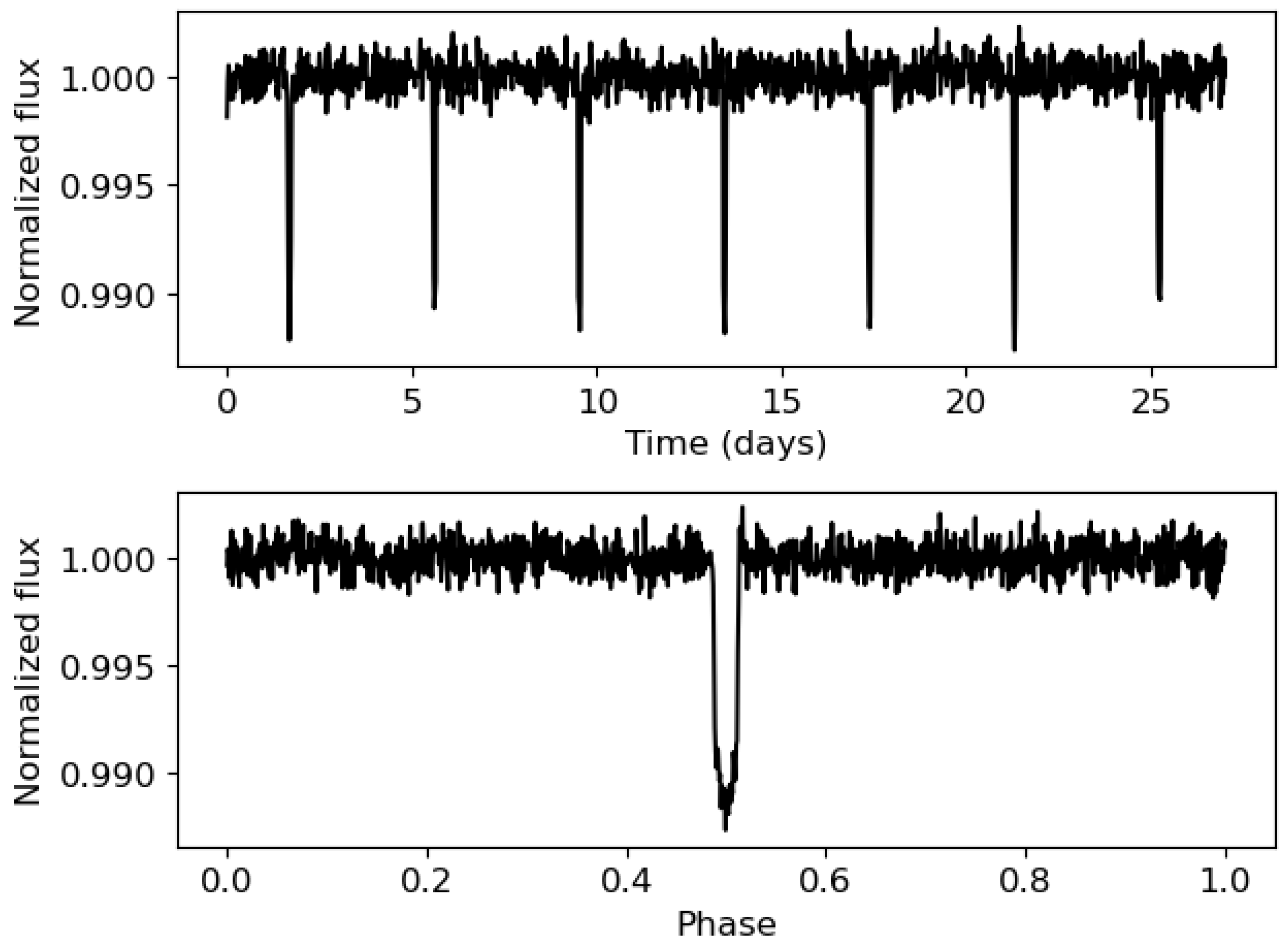
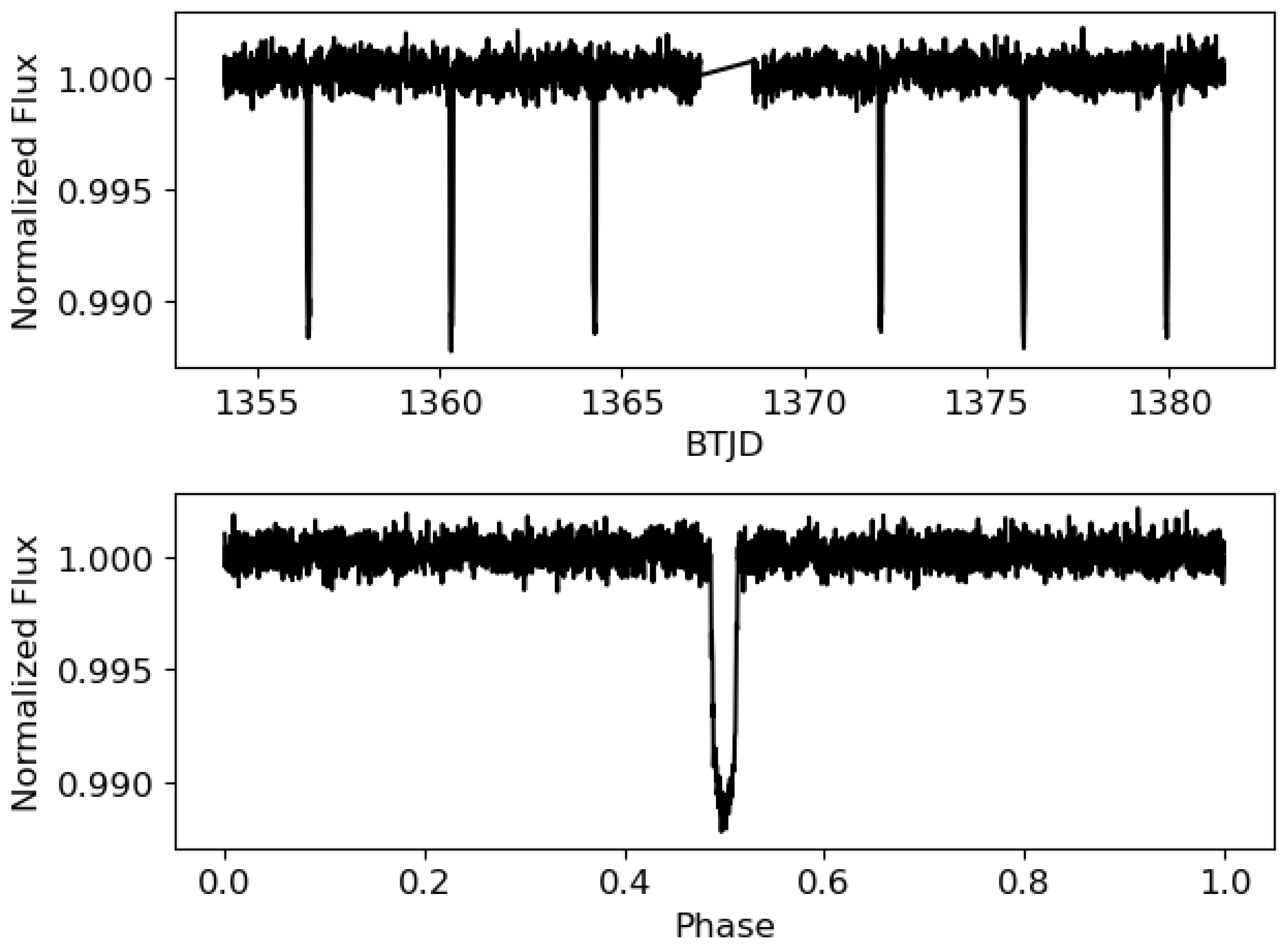
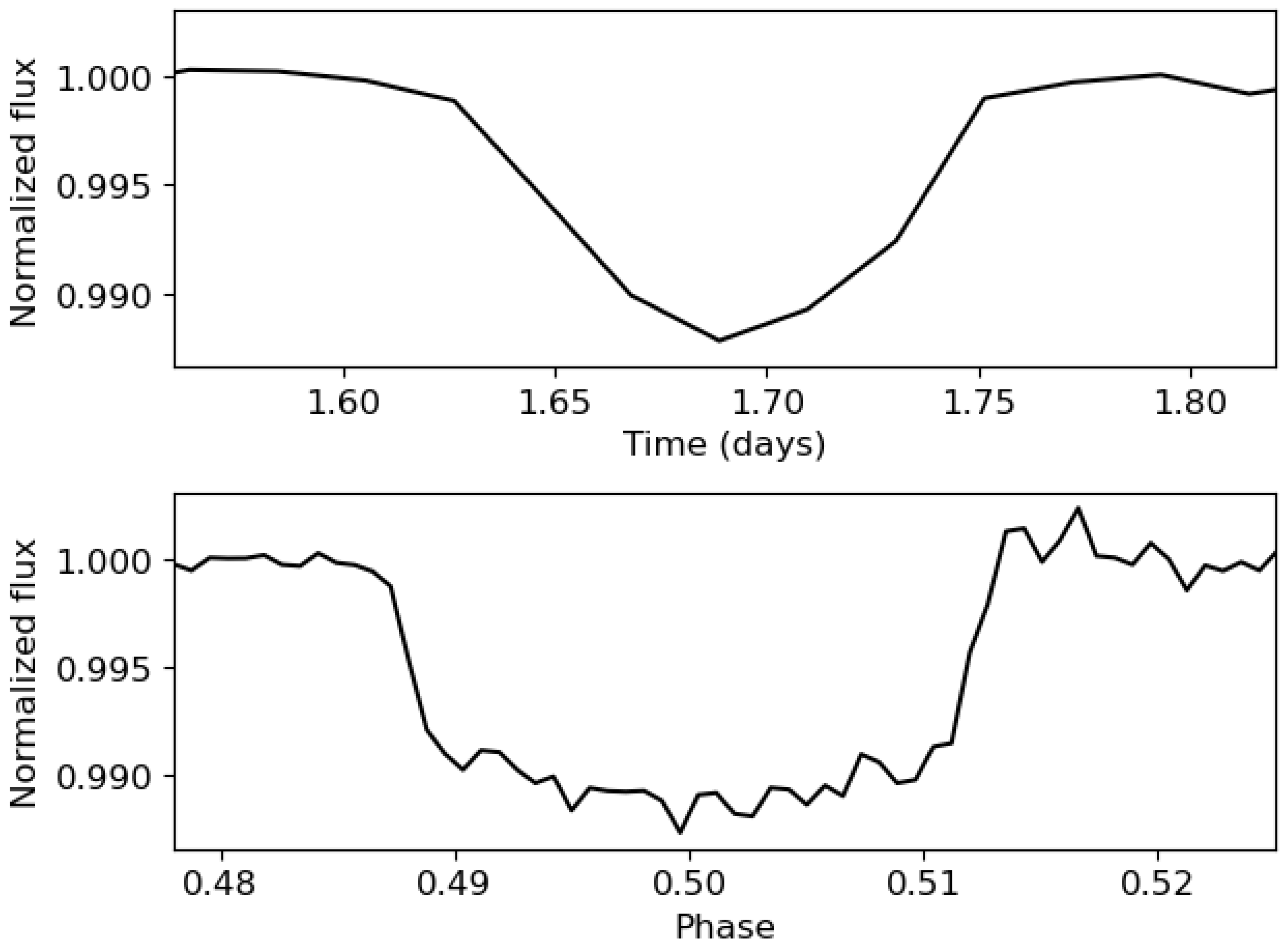
An example of the 2 views (complete and phase-folded) of a simulated light curve is shown in Figure 3. As shown, a phase-folded light curve allows for obtaining a better transit shape. For checking this, a zoom of Figure 3 is shown in Figure 4. As shown, the transit of the phase-folded light curve is composed of much more points, thus allowing for better checking the Mandel and Agol theoretical shape. Both views of the light curve were simulated, taking into account the main parameters from TIC 183537452 (TOI-192), except the epoch and the temporal span of the light curve, which were not considered as they do not condition the noise levels and the transit shape. TOI-192 is part of the TOI Catalog, short for the TESS Objects of Interest Catalog, which comprises a compilation of the most favorable targets for detecting exoplanets. Its complete and phase-folded light curves are shown in Figure 5. TESS light curves exhibit gaps that occur during the data download by the telescope. However, this phenomenon was not considered because either no transits are lost in the gap, and thus, the separation between two consecutive transits is maintained, or if any transits are in this zone, the distance between the last transit before the gap and the next one after the gap will be separated by a temporal distance proportional to the orbital period, so the calculation of this value will not be affected. Aside from this, the simulated light curves closely resemble those expected from TESS, showing similar noise levels for similar stellar magnitudes and showing a similar transit depth similar to ${\left(R_p\left[R_{★}\right]\right)}^2$.

The training process (see Section 3) requires 2 different datasets, as it is important to test both models in order to check their generalization to data unknown for the CNN (this is known as test process). Thus, a train dataset with 650,000 light curves and a test dataset with 150,000 were developed. The number of light curves in the train dataset was chosen after training both models a large number of times and increasing the number of light curves used. The final amount of light curves corresponds to the one with which the best results were obtained. Above this number, significant improvement was seen. In addition, the number of light curves in the test dataset was chosen to have a large statistic that would allow a good check of the results.

2.3. Convolutional Neural Networks (CNNs): Our 1D CNN Models

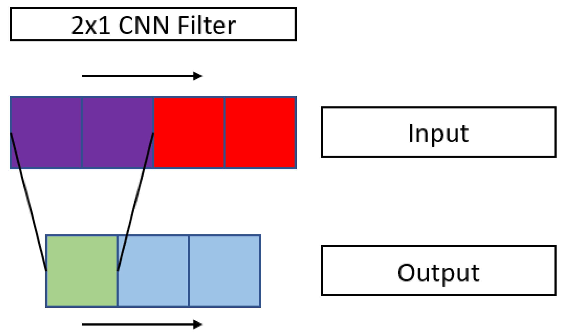
The transit shape previously shown differs from an outlier or the noise present in light curves only by their shape. This is why CNNs play a crucial role in transit detection and characterization, as these algorithms could distinguish between both signals (noise and transits), even though they are at similar levels.

CNNs apply filters to the input data that allow the detection of different features that characterize them. An example of a 1D CNN filter is shown in Figure 6.

The main activation function used in this research is known as parametric rectifier linear unit (PReLU) [36]. If $y_i$ is considered as the input of the non-linear activation function, its mathematical definition is:

$$f\left(y_i\right)=\left\{\begin{array}{cc}{y}_i\hfill & \hfill if{y}_i>0\\ a_i·y_i\hfill & \hfill if{y}_i\le 0\end{array}\right..$$

(8)

The main difference between this activation function and the rectifier linear unit (ReLU) [37], which is one of the most commonly used, is that, in ReLU, $a_i$ is equal to 0, while in PReLU, it is a learnable parameter.

The gradient of this function when optimizing with backpropagation [38] is (taking into account a derivative with respect to the new trainable parameter, $a_i$)

$$\frac{\mathsf{\partial }f\left(y_i\right)}{\mathsf{\partial }{a}_i}=\left\{\begin{array}{cc}0\hfill & \hfill if{y}_i>0\\ y_i\hfill & \hfill if{y}_i\le 0\end{array}\right..$$

(9)

Our CNN model consists, actually, in two 1D CNN models, as a transit analysis could be understood as a temporal series one. The main fact is that flux vectors of the simulated light curves were used as inputs for training, validating, and testing them (see Section 3). All the processes were carried out in Keras [39]. The first model (it will be referred to as model 1 from now on) works with complete light curves and is able to predict the value of the orbital period of the transit-like signals. The second model (it will be referred to as model 2 from now on) works with phase-folded light curves and is able to predict ${\left(R_p\left[R_{★}\right]\right)}^2$ and $a\left[R_{★}\right]$. The model predicts ${\left(R_p\left[R_{★}\right]\right)}^2$ instead of $R_p\left[R_{★}\right]$ because the squared value is related to the transit depth.

The structure of both models is the same with the difference of the last layer, which has the same number of neurons as the number of parameters to predict. Both models are composed of a 4-layer convolutional part and a 2-layer multilayer perceptron (MLP) part. In the convolutional part, all the layers have a filter size of 3 and have 2 strides. The numbers of convolutional filters are, respectively, 12, 24, 36, and 48. All the layers are connected by a PReLU activation function and have the padding set to the same, which avoids the change of the shape of the light curves among the layers due to the convolutional filters. The MLP part is composed of a layer with 24 neurons activated by PReLU and a last layer with 1 neuron for model 1 and 2 neurons for model 2, without an activation function. The two parts of the models are connected by a flatten layer. A scheme of model 1 is shown in Figure 7. The scheme of the second model consists of changing the number of neurons to 2 in the last layer (2nd sense).

3. Model Training and Test Results and Discussion

First of all, both processes were carried out on a server with an Intel Xeon E4-1650 V3, 3.50 GHz, with 12 CPUs (6 physical and 6 virtual). It had a RAM of 62.8 Gb.

As both models are 1D CNN models, it is important to preprocess the input light curves due to the fact that convolutional filters usually take the maximum value on them, which would entail the loss of the transits. Thus, the light curves were inverted and set between 0 and 1.

In addition, the values related to the parameters that the 1D CNN models were learning to predict (from now on, it will be referred as labels) were normalized. The following transformation was applied to each label, supposing max_labels as the maximum of all the labels simulated and min_labels the minimum value:

$$label=\frac{label-min\_labels}{max\_labels-min\_labels}.$$

(10)

These transformations set the data between 0 and 1. This is necessary because deep learning techniques work more properly when the input and output data are normalized.

Before training both models, adaptive moments (Adam) [40] were selected as the optimizer. Adam is a stochastic gradient descent (SGD) [41] method that changes the value of the learning rate using the values of the first- and second-order gradients. The initial learning rate was set to 0.0001 (chosen after many training processes). As a loss function, the mean squared error (MSE) was chosen.

One of the main parts of the training process consists in validating the model train with a dataset different from the one used for updating the hyperparameters in each epoch (an epoch is each time the training dataset is used to train the model) in order to check how well the model is being generalized during the training process. Keras allows for performing that with a parameter known as validation split. A number between 0 and 1 that refers to the percentage of the train dataset is used for this process. A proportion of 30% of the dataset was split; i.e., a validation split of 0.3 was selected. Furthermore, a batch size of 16 was selected. For monitoring the training, the MSE loss function was chosen. Each epoch took about 200 s to be completed in our server.

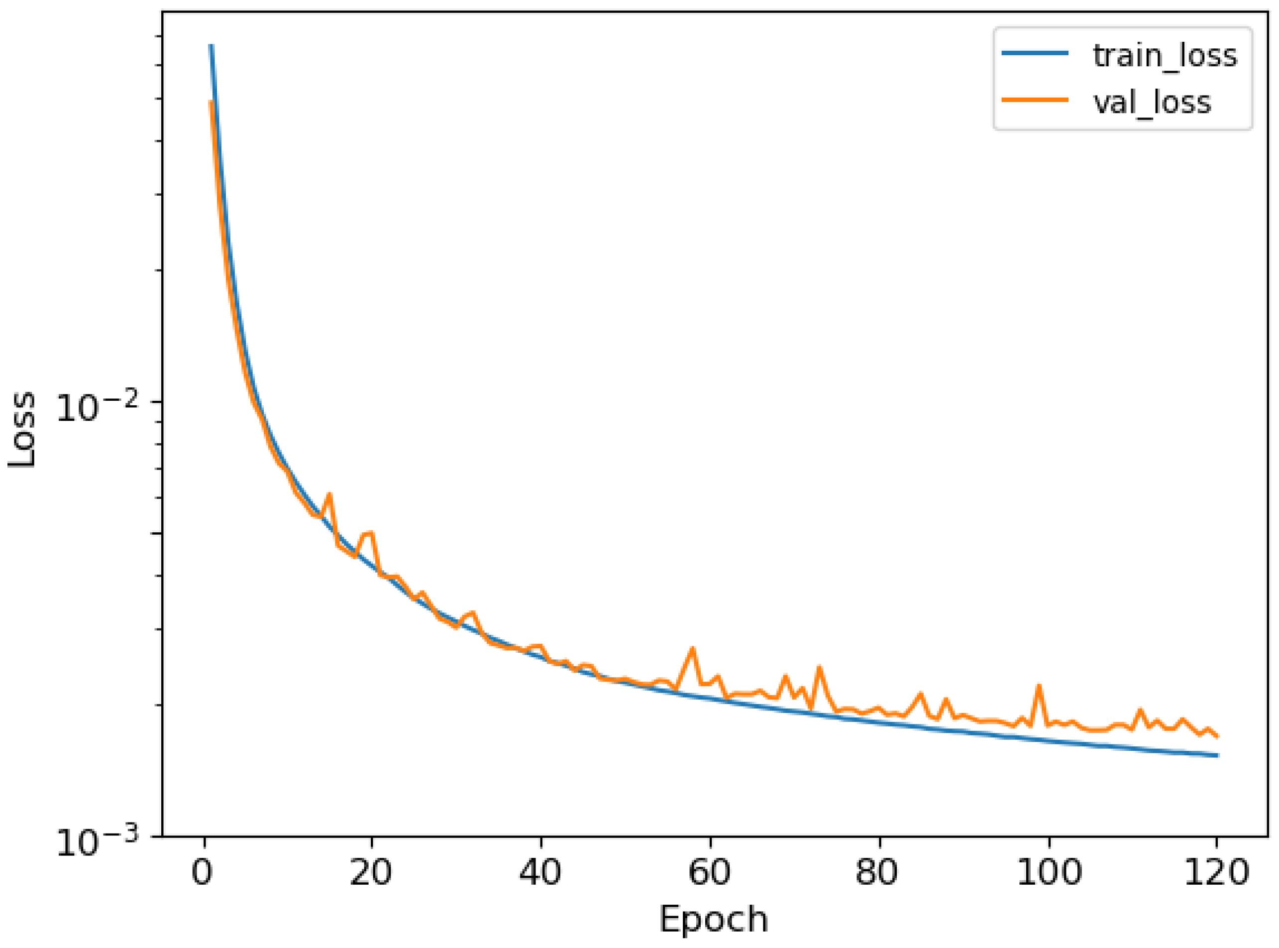
After training both models, the training histories were obtained, in which training and validation loss were plotted against the epochs. Figure 8 and Figure 9 show, respectively, the training history of models 1 and 2 in a logarithmic scale. As shown, the training process was completed correctly, as the validation loss decreased along with the training loss among the epochs.

The test process was carried out with the test dataset composed by 150,000 light curves (as explained in Section 2.2). The accuracy of the predictions was studied with a comparison between them and the values with which the light curves were simulated. Theoretically, the perfect result would be adjusted to a linear function with a slope 1 and an intercept of 0. The results were fit with a linear regression and obtained $R^2=0.991$ for the orbital period (model 1), $R^2=0.974$ for ${\left(R_p\left[R_{★}\right]\right)}^2$ (model 2), and $R^2=0.971$ for $a\left[R_{★}\right]$ (model 2). These results mean that most of the data predicted are in agreement with the simulated data, which implies that our 1D CNN models are properly predicting the planetary parameters. Furthermore, the mean absolute error (MAE) was computed for both models, obtaining $MAE=0.015d$ for the orbital period (model 1), $MAE=0.0003$ for ${\left(R_p\left[R_{★}\right]\right)}^2$ (model 2), and $MAE=0.9113$ for $a\left[R_{★}\right]$ (model 2). 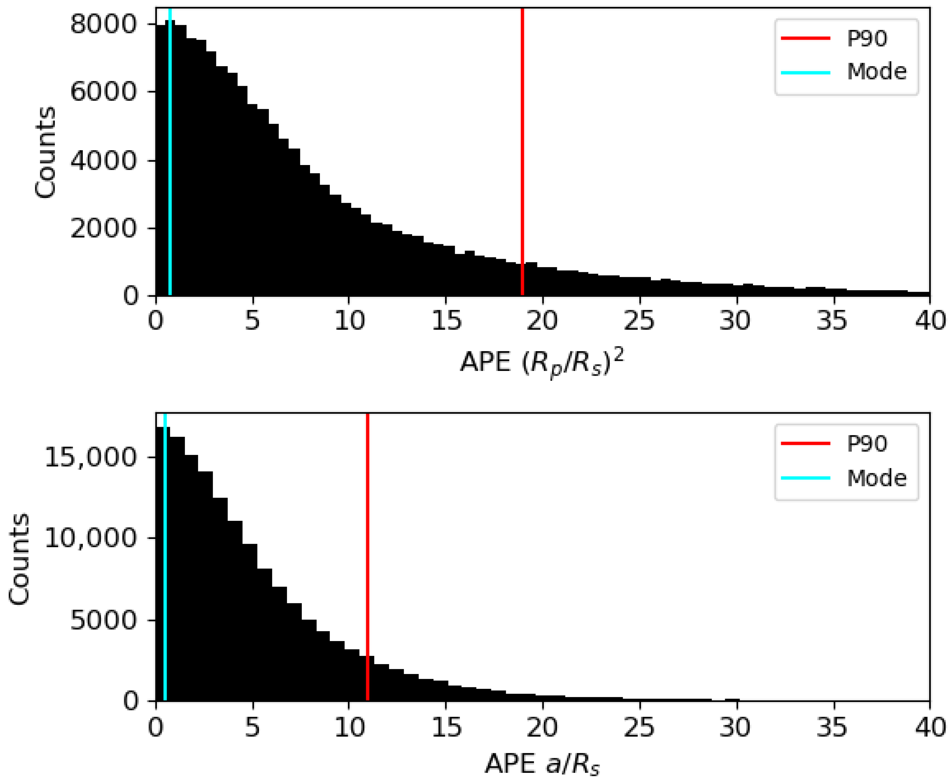These results could be better understood with the plot of a small randomly chosen sample of 100 predictions and test data (see Figure 10 and Figure 11) because the total plot of the data is a bit clumpy and could make the results confusing. As shown, the predictions fit correctly to the simulated ones. In addition, as an absolute error could be a bit confusing, the absolute percentage error (APE) was computed from all the predictions and the obtained value were plotted in histograms, in this case, with the whole data (see Figure 12 and Figure 13, which make reference, respectively, to models 1 and 2). The values of the modes from the histograms of $P\left(d\right)$, ${\left(R_p\left[R_{★}\right]\right)}^2$ and $a\left[R_{★}\right]$ are, respectively, 0.003, 0.69, and 0.38. To sum up all the results, all of them are shown in

Table 3. Statistics computed with the predictions of the test process for each of the predicted parameters (P(d), ${\left(R_p\left[R_{★}\right]\right)}^2$, and $a\left[R_{★}\right]$).

Parameter	MAE	${\mathit{R}}^2$	Histogram Mode (%)	Histogram P90 (%)
P(d)	0.015	0.99	0.7	7.5
${\left(R_p\left[R_{★}\right]\right)}^2$	0.0003	0.97	0.8	19
$a\left[R_{★}\right]$	0.91	0.97	0.5	11

.

All these results show that both models properly predict the parameters P, ${\left(R_p\left[R_{★}\right]\right)}^2$ and $a\left[R_{★}\right]$, with low uncertainties. In addition, they show that both models properly generalize without generating dependence on the train dataset. Among other previous studies, these results show that 1D CNN is a good choice not only for checking if a light curve presents transit-like signals but also for estimating parameters related to its shape. The test dataset shows a wide range of values, but even so, the models do not show any bias in the results (which would mean that the models predict better in some regions than in others), which means that the models are properly trained. To put these results in context, 10,000 light curves from the test dataset were analyzed with TLS and the $MAE$ for $P\left(d\right)$ and ${\left(R_p\left[R_{★}\right]\right)}^2$ were computed respect to the values with which the light curves were simulated (TLS does not compute the semimajor axis of the orbit). The obtained values are, respectively, $0.009$ and $0.0018$, which mean that our CNN models predict all the parameters with a similar precision compared with the most used algorithms nowadays.

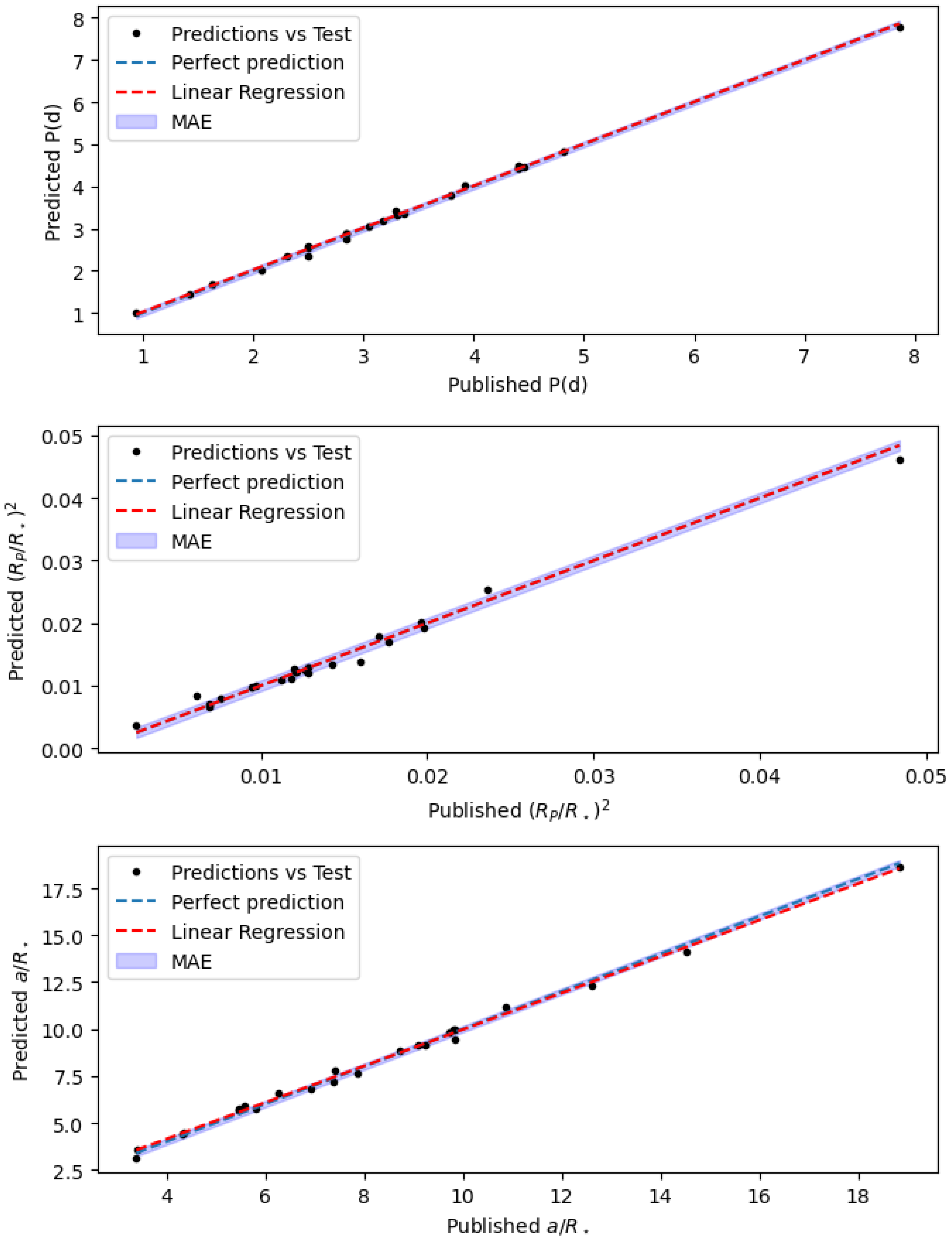
The models were also tested on real TESS data. From the Mikulski Archive for Space Telescopes (MAST) (bulk download https://archive.stsci.edu/tess/bulk_downloads/bulk_downloads_ffi-tp-lc-dv.html (accessed on 1 December 2023)), 25 light curves with confirmed transiting exoplanets from the stars part of the candidate target lists (CTLs) [42], which is a special subset from the TESS Input Catalog (TIC) containing targets that are good for detecting planetary-induced transit-like signals, were obtained. This subset of light curves was decided to be used because there are preprocessed and corrected light curves available to download from all of them. All the light curves were analyzed with our 1D CNN models, and the results were compared with their published values from [29]. The phase-folded light curves were computed with the predicted value of the orbital period. From the results, the MAE, $R^2$, and Mean Absolute Percentage Error (MAPE) were computed. All the predicted and real values are shown in

Table 4. Published and predicted parameters of exoplanets observed by TESS. The first two columns show, respectively, the TIC id of the star and the sector in which each light curve was obtained. The other columns show the published parameters, the predicted parameters, the AE, and the APE of each of the parameters and exoplanets. Published data were obtained from ExoFOP.

TIC id	Sector	P(d) Real	P(d) Pred	AE (P(d))	APE (P(d)) (%)	${\left({\mathit{R}}_{\mathit{P}}\left[{\mathit{R}}_{\mathbf{★}}\right]\right)}^2$ Real	${\left({\mathit{R}}_{\mathit{P}}\left[{\mathit{R}}_{\mathbf{★}}\right]\right)}^2$ Pred	AE $\left({\left({\mathit{R}}_{\mathit{P}}\left[{\mathit{R}}_{\mathbf{★}}\right]\right)}^2\right)$	APE $\left({\left({\mathit{R}}_{\mathit{P}}\left[{\mathit{R}}_{\mathbf{★}}\right]\right)}^2\right)(\mathbf{\%})$	$\mathit{a}\left[{\mathit{R}}_{\mathbf{★}}\right]$ Real	$\mathit{a}\left[{\mathit{R}}_{\mathbf{★}}\right]$ Pred	AE $\left(\mathit{a}\left[{\mathit{R}}_{\mathbf{★}}\right]\right)$	APE $\left(\mathit{a}\left[{\mathit{R}}_{\mathbf{★}}\right]\right)(\mathbf{\%})$
183537452	2	3.9230	4.0200	0.0970	2.4726	0.0094	0.0098	4.2553	4.2553	12.6200	12.3000	0.3200	2.5357
158623531	2	7.8600	7.7900	0.0700	0.8906	0.0127	0.0125	1.2598	1.2598	14.5200	14.1000	0.4200	2.8926
100100827	2	0.9414	1.0150	0.0736	7.8181	0.0097	0.0100	3.0928	3.0928	3.3900	3.1500	0.2400	7.0796
388104525	2	2.4997	2.5762	0.0765	3.0604	0.0128	0.0130	1.5625	1.5625	7.4200	7.7900	0.3700	4.9865
149603524	2	4.4119	4.4986	0.0867	1.9651	0.0121	0.0122	1.0744	1.0744	5.5700	5.9000	0.3300	5.9246
184240683	2	1.6284	1.6700	0.0416	2.5547	0.0122	0.0123	0.6987	0.6987	3.3970	3.5800	0.1830	5.3871
38846515	2	2.8494	2.7500	0.0994	3.4885	0.0069	0.0071	3.0316	3.0316	5.4800	5.6600	0.1800	3.2847
230982885	2	2.0728	2.0000	0.0728	3.5122	0.0112	0.0108	3.5714	3.5714	9.7300	9.8500	0.1200	1.2333
149603524	1	4.4119	4.4600	0.0481	1.0902	0.0121	0.0121	0.3306	0.3306	6.2800	6.5600	0.2800	4.4586
38846515	1	2.8494	2.8800	0.0306	1.0739	0.0069	0.0065	5.7971	5.7971	9.8376	9.9961	0.1585	1.6113
388104525	3	2.4997	2.3400	0.1597	6.3888	0.0118	0.0111	5.9322	5.9322	9.8300	9.4600	0.3700	3.7640
149603524	3	4.4119	4.4285	0.0166	0.3763	0.0120	0.0128	6.6667	6.6667	10.8700	11.1500	0.2800	2.5759
268766053	3	3.3100	3.3600	0.0500	1.5106	0.0177	0.0169	4.4604	4.4604	5.4800	5.6700	0.1900	3.4672
388104525	4	2.4998	2.5340	0.0342	1.3681	0.0129	0.0121	5.9829	5.9829	7.3800	7.1654	0.2146	2.9079
38846515	4	2.8493	2.8803	0.0310	1.0880	0.0069	0.0068	1.8813	1.8813	9.8200	9.9600	0.1400	1.4257
289793076	1	3.0440	3.0548	0.0108	0.3548	0.0197	0.0201	2.2380	2.2380	9.2500	9.1300	0.1200	1.2973
300871545	1	4.8170	4.8450	0.0280	0.5813	0.0236	0.0253	6.9915	6.9915	5.8100	5.7300	0.0800	1.3769
231663901	1	1.4300	1.4292	0.0008	0.0559	0.0198	0.0192	3.0303	3.0303	5.4800	5.7800	0.3000	5.4745
234523599	1	3.7960	3.7940	0.0020	0.0527	0.0484	0.0462	4.5455	4.5455	18.8400	18.6500	0.1900	1.0085
290131778	1	3.3089	3.3167	0.0078	0.2357	0.0025	0.0036	44.0000	44.0000	4.3300	4.4250	0.0950	2.1940
97409519	1	3.3729	3.3406	0.0323	0.9576	0.0160	0.0138	13.7500	13.7500	9.1100	9.1820	0.0720	0.7903
281459670	1	3.1740	3.1857	0.0117	0.3698	0.0143	0.0134	6.2456	6.2456	8.7200	8.8100	0.0900	1.0321
260609205	1	4.4620	4.4711	0.0091	0.2035	0.0171	0.0179	4.6784	4.6784	6.9200	6.8200	0.1000	1.4451
25155319	1	3.2890	3.4147	0.1257	3.8214	0.0061	0.0085	38.4365	38.4365	7.8800	7.6500	0.2300	2.9188
25375553	1	2.3110	2.3500	0.0390	1.6876	0.0076	0.0080	5.6150	5.6150	4.3500	4.5000	0.1500	3.4483

, along with the APE and the Absolute Error (AE) computed for each of the parameters. The obtained MAEs of P(d), ${\left(R_p\left[R_{★}\right]\right)}^2$, and $a\left[R_{★}\right]$ are, respectively, $0.0502$, $0.0004$, and $0.20$; the MAPE of P(d), ${\left(R_p\left[R_{★}\right]\right)}^2$, and $a\left[R_{★}\right]$ are, respectively, $1.87\%$, $7.16\%$, and $2.98\%$; and the $R^2$ values from $P\left(d\right)$, ${\left(R_p\left[R_{★}\right]\right)}^2$, and $a\left[R_{★}\right]$ are, respectively, $0.981$, $0.978$, and $0.985$. These results mean that our 1D CNN models also perform properly on real data. In Figure 14, the comparison between real data and predicted values is plotted to check the accuracy of the predictions visually. The differences between the results obtained with real and simulated data were due to the fact that, although simulating the light curves as most similar as possible to those expected for the TESS mission was attempted, in reality, it is impossible to have them the same. However, these results show that both models are able to characterize transiting exoplanets from the TESS light curves of their host star also in real data, which means that our models were well trained and that the light curve simulator is able to mimic real TESS light curves with high accuracy.

In addition, is important to remark that analyzing 150,000 light curves for each model took 30 s to complete, which is similar to three times the time required for analyzing 1 light curve with TLS in our server. TLS aims to maximize transit-like signal detection while decreasing the executing time as much as possible. However, as least squares algorithms allow for choosing different prior parameters, the amount of time required considerably depends on the density of the priors. For example, the minimum depth value considered during the analysis or the period intervals in which to search for periodic signals considerably constrain the execution time to complete the analysis. In addition, the light curves’ length (in points) and their time span have also high impact. As shown in [6], the executing times quadratically depend on the time span of the light curve. Obviously, the computation power available is also fundamental for reducing the computing times. They show that on an Intel Core i7-7700K, a mean 4000-points-length K2 [43] light curve takes about 10 s. This process would probably not be possible with current algorithms in common computing facilities if the dataset that has to be analyzed would be composed of many thousands of stars (as the ones provided by current observing facilities), because current algorithms are highly time-consuming, and also, they need a high computational cost, which is not always available.

Apart from reducing the computational cost and time consumption, our approach avoids the data preparation that is required from current MCMC and least squares methods. Almost all of them require obtaining some parameters related to the star, such as the limb darkening coefficients, something that could be carried out with different algorithms, which need stellar information, such as the effective temperature ($T_{eff}$), the metallicity ($[M/H]$), and microturbulent velocity, among others. Is not always easy to obtain these parameters from stellar databases or to compute them, especially if the analysis is carried out on a dataset composed of many thousands of stars, as the ones provided by current observing facilities. However, our 1D CNN models allow for determining all these parameters in real time only by applying a simple normalization to the input data in order to invert the light curves and to set them between 0 and 1.

4. Conclusions

In this research, we went one step further than our previous work. The light curve simulator was generalized to TESS data, and was also modified to obtain phase-folded light curves (in addition to the complete ones) with Gaussian noise, mimicking those expected for TESS data. As light curve data can be understood as temporal series and also the predictions have high shape dependency, it was thought that 1D CNN techniques would be the most accurate ML techniques as they learn from the input data due to the convolutional filters and they perform properly with temporal series data.

Our two models are similar, but changing the last layer to adjust them to the required output values. The first model works with complete light curves and thus predicts the value of the orbital period. The second model works with phase-folded light curves and estimates the values ${\left(R_p\left[R_{★}\right]\right)}^2$ and $a\left[R_{★}\right]$.

The training process was carried out with a dataset of 650,000 light curves, but splitting 30% of them to validate the training. The training histories show correct performance of both processes (training and validation), where both of them decrease among the epochs without the existence of a huge difference between them (that would suppose overfitting). After training both models, another dataset composed of 150,000 light curves was used to test the results with a set different from the one used for training it (the test dataset). The most visual way to analyze the accuracy of the prediction is by plotting the predicted values against the simulated ones. In addition, some statistics that allow for taking into account the average error with which the CNN predicts the values were computed. More concretely, the mean average error (MAE) and a linear regression $R^2$ coefficient were considered. For the orbital period, $MAE=0.015d$ and $R^2=0.980$ were obtained (predictions made with model 1). For ${\left(R_p\left[R_{★}\right]\right)}^2$, $MAE=0.0003$ and $R^2=0.974$ were obtained (predictions made with model 2). For $a\left[R_{★}\right]$, $MAE=0.9113$ and $R^2=0.971$ were obtained (predictions made with model 2). The values of the modes from the histograms computed with the absolute percentage errors (APEs) of $P\left(d\right)$, ${\left(R_p\left[R_{★}\right]\right)}^2$, and $a\left[R_{★}\right]$ are, respectively, 0.003, 0.69, and 0.38. Apart from that, a set of 10,000 light curves from the test dataset was analyzed with TLS, showing that both models characterize planetary systems from their host star light curves with similar accuracy compared with current algorithms. In addition, both models were tested on real data obtained of CTL light curves from MAST. The results obtained for $P\left(d\right)$, $R_p\left[R_{★}\right]$, and $a[R_{★}]$ ($0.0502$, $0.0004$, and $0.20$, respectively, of the MAEs; $1.87\%$, $7.16\%$, and $2.98\%$, respectively, of the MAPEs; and $0.98$, $0.976$, and $0.985$, respectively, of $R^2$), show that both models are able to characterize planetary systems from TESS light curves with high accuracy, which means not only that they are well trained and thus can be used for characterizing new exoplanets from TESS mission, but also that the light curve simulator is able to mimic with high fidelity the light curves expected from this mission. In addition, our models reduce the computing time and computational cost required for analyzing such large datasets as the ones available from current observing facilities; more concretely, our models take 30 s to complete the analysis of the test dataset (150,000 light curves), which is similar to three times the time required for analyzing a single light curve with TLS. Moreover, with our models it is not necessary to set the priors in which to compute the main parameters, which also increases the time consumption.

In addition, we are not only in agreement with the fact that CNN in general and 1D CNN in particular are a good choice for analyzing light curves trying to search for transiting exoplanets (as previous research do [20,21,22,23,24,25,26,27,28]), but also that CNN algorithms are able to characterize planetary systems with high accuracy in a short period of time.