A Kuramoto Model for the Bound State Aharonov–Bohm Effect

Abstract

The Aharonov–Bohm effect can be described as a phase difference in interfering charged particles that travel through two distinct pathways oppositely surrounding a perpendicularly-positioned solenoid. The magnetic field emanates from the solenoid but does not intersect the pathways. On the other hand, the Kuramoto model can be used to identify the synchronization conditions that lead to a particular phase difference by treating the phases as coupled oscillators. Starting with the overall wave function expression for the electron in an Aharonov–Bohm potential, we derive a version of the Kuramoto model describing the phase dynamics of the bound state of the quantum mechanical system. We show that the resulting synchronization condition of the model coincides with the allowable values of the flux parameter for our case to achieve an Aharonov–Bohm effect.

1. Introduction and Motivation

The Aharonov–Bohm (AB) effect [1], which is an interference phenomenon, continues to exhibit quantum mechanical features that have not yet been fully understood, e.g., the anomalous AB interference in a quantum Hall Fabry–Pérot interferometer as observed in Ref. [2], the time-dependent AB effect and the absence of its apparent experimental evidence (as also mentioned in a recent study Ref. [3]), the topological nature of the AB effect (see, e.g., a recent study that challenges its conventional concept in Ref. [4]). On the other hand, the Kuramoto model (KM) [5] has been applied to many branches of science (see review papers, e.g., Refs. [6,7,8]) but scarcely to quantum mechanics. For quantum applications of the KM, see the examples given in Refs. [9,10,11,12]. Describing the AB effect from the KM’s perspective is, therefore, of interest and not considered elsewhere.

Synchronizations in quantum systems have recently been studied based on either having a classical analog (see, e.g., Refs. [13,14]) or none at all, e.g., Ref. [15]. Furthermore, synchronizations of interfering particles, such as between photons (see, e.g., Ref. [16]) and between electrons (see, e.g., Ref. [17]) have also been considered. Since the synchronization condition is a main characteristic of the KM, it is, therefore, of particular interest to use the model to study the synchronization conditions of the bound state AB effect and their relationship with the interference occurring within the quantum system. Alongside the synchronization conditions, we are also interested in determining the extent of the magnetic field region near the interference line of the AB effect.

In this letter, beginning with the general case of the AB effect [1], we consider its simplest case, the bound state, by constraining the path taken by the electron to that of a circle with constant radius, e.g., Refs. [18,19,20]. Then, with its known interference phase difference and wave functions (see, e.g., Ref. [1]), we propose a version of the KM and study the phase dynamics of the system.

2. A Kuramoto Model for the System

Begin with a KM model of the form [5]

$${\dot{\sigma }}_i:={\displaystyle \frac{\mathrm{d}{\sigma }_i}{\mathrm{d}t}}={\omega }_i+{\displaystyle \frac{K}{N}}\sum _{j=1}^{N}sin\left({\sigma }_j-{\sigma }_i\right),$$

(1)

where ${\sigma }_i={\sigma }_i\left(t\right)$ is the phase of the phase oscillator i (with $i=1,2,\dots ,N$) as a function of time $t\ge 0$, ${\omega }_i$ its angular frequency, K a uniform coupling strength coefficient and N the total number of phase oscillators.

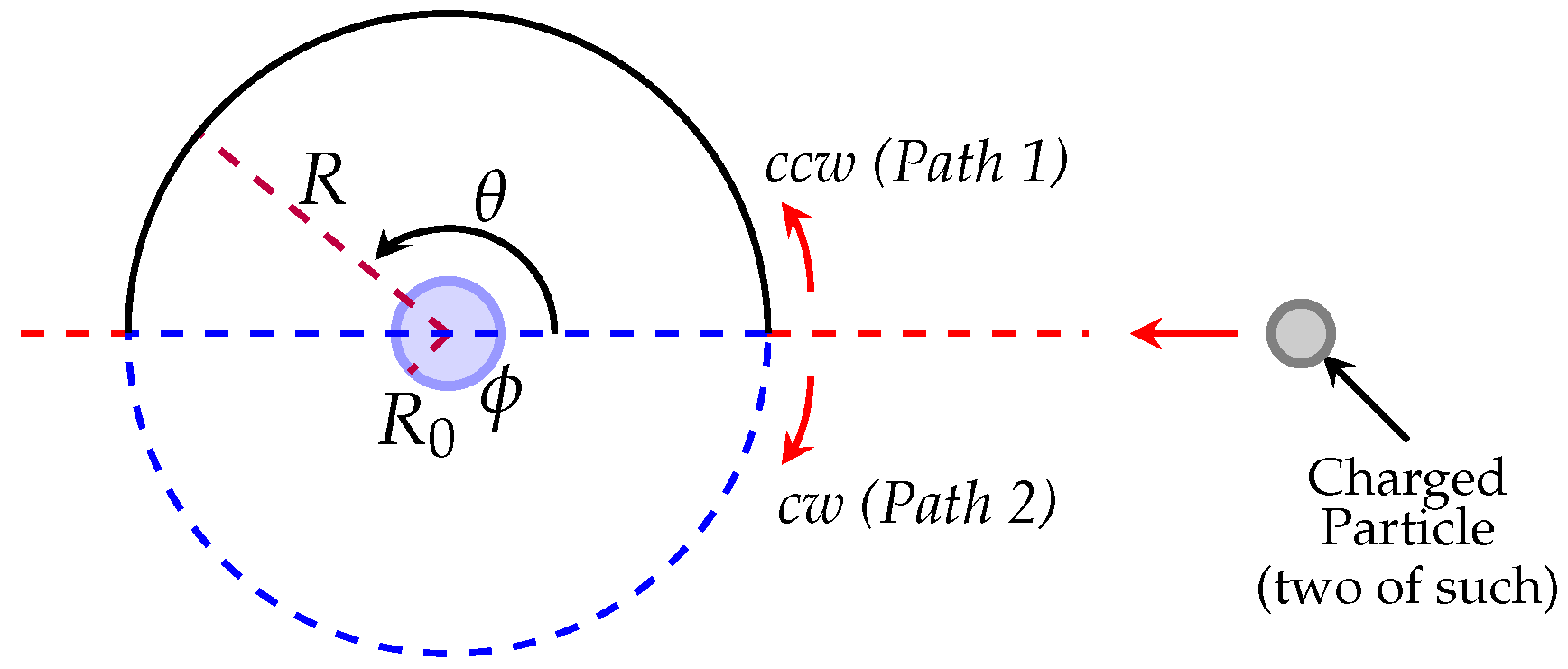
Consider now a two-electron system, with each electron initially in the angular position ${\theta }_0:=\theta \left(0\right)=0$ moving along a circular path of constant radius $R,$ one in the upper semicircle and the other in the lower semicircle; see Figure 1. The two paths, namely, Path 1 and Path 2, form a circular ring except at the endpoint $\theta \left(t\right)=\pi$.

In the center of the ring, there is an AB effect source, a magnetically impenetrable solenoid of radius $R_0$ oriented perpendicular to the semicircular paths and generating a magnetic field of flux $\varphi$. The resulting magnetic field lines emerge from the top, flow down the sides of the solenoid beyond the trajectories, and return through the bottom. Since this magnetic field does not intersect the paths of the electrons, the paths (of radius $R\gg R_0$) of the electrons are in a region where the magnetic field is excluded. Consequently, there is a phase shift between the electron trajectories at their mutual endpoint, specifically at $\theta \left(t\right)=\pi$.

In the general case where the “detecting” particles (i.e., the charged particles moving along the semicircular paths that will sense the AB effect) have charge $le,l\in \mathbb{Z}\setminus \left\{0\right\}$, the phase difference between Path 1 and Path 2 when they interfere at $\theta \left(t\right)=\pi$, is [1,18]

$${\sigma }_1-{\sigma }_2={\displaystyle \frac{S_1-S_2}{\hslash }}=2\pi \alpha ,\alpha :={\displaystyle \frac{le\varphi }{2\pi \hslash c}};$$

(2)

where $S_i$ represents the action of the classical Path i, ℏ the reduced Planck’s constant, and c the speed of light in vacuum. In Equation (2), it is observed that the interference depends on the phase difference by a factor of $2\pi$. This specifically entails that, when the parameter $\alpha$ (called the flux parameter) is shifted by an integer value, the interference phenomenon remains completely “unaffected”. Thus, $\alpha$ only takes specific discrete values of $\varphi =({\varphi }_0/n),n\in \mathbb{Z}\setminus \left\{0\right\}$, where ${\varphi }_0:=2\pi \hslash c/e$ (known as the quantum of flux or London’s unit) and $ne$ is the charge used by the “source” of the magnetic flux in the solenoid, e.g., Refs. [1,18]. In particular, with $\alpha =l/n$, the AB effect is detectable only for $\{l/n\}$, where $\{·\}$ represents the fractional part of the number. In our case, where $l=-1$, the AB effect is detectable whenever $\left|n\right|\ne 1$. We can find a detailed theoretical description in Refs. [1,18] and some supporting experiments in the works [21,22].

Hence, with $N=2$, i.e., for Paths 1 and 2 in Figure 1, Equation (1) gives

$${\dot{\sigma }}_1={\omega }_1+{\displaystyle \frac{K}{2}}sin\left({\sigma }_2-{\sigma }_1\right),$$

(3)

and

$${\dot{\sigma }}_2={\omega }_2-{\displaystyle \frac{K}{2}}sin\left({\sigma }_2-{\sigma }_1\right).$$

(4)

This study aims to determine ${\omega }_1$, ${\omega }_2$, and K. To do so, we make the following assumptions:

• The probability for an electron to take either of the two paths is the same;
• The two electrons simultaneously start at ${\theta }_1\left(t_0\right)={\theta }_2\left(t_0\right)=0$, one then proceeds towards the end of the semicircular track through Path 1 and the other through Path 2;
• The electrons travel the same amount of angular displacement $\theta :=\theta \left(t\right)$ (differing only in the sign of $\theta$), at the time interval $t-t_0=t,$ thus enabling them to interfere as $\left|\theta \right(t\left)\right|\to \pi$.

Now, in quantum mechanics, the wave function $\psi \left(t\right)$ for the (bound state) Aharonov–Bohm effect can be expressed in terms of $S_1$ and $S_2$ as [1]

$$\psi \left(t\right)={\psi }_1^0\left(t\right){\mathrm{e}}^{-(\mathrm{i}/\hslash )S_1}+{\psi }_2^0\left(t\right){\mathrm{e}}^{-(\mathrm{i}/\hslash )S_2},$$

(5)

where ${\psi }_i^0$ denotes the wave function for the free particle moving along path i. Furthermore, since this system also undergoes a scattering process [1], then $\psi$ can further be expressed in terms of the incident wave function ${\psi }_{\mathrm{inc}}$ and the scattered wave function ${\psi }_{\mathrm{scatt}}$ as [1]

$$\psi \left(t\right)={\psi }_{\mathrm{inc}}\left(t\right)+{\psi }_{\mathrm{scatt}}\left(t\right),$$

(6)

where, for $\left|\theta \right|<\pi \iff \left|\theta \right(t\left)\right|<\pi$, $\forall t\ge 0$,

$${\psi }_{\mathrm{inc}}\left(t\right):={\mathrm{e}}^{-\mathrm{i}\left(\alpha \theta \left(t\right)+Rkcos\left(\theta \right(t\left)\right)\right)},$$

(7)

and

$${\psi }_{\mathrm{scatt}}\left(t\right):={\displaystyle \frac{sin\left(\pi \alpha \right)}{\sqrt{2\pi \mathrm{i}Rk}cos(\theta \left(t\right)/2)}}{\mathrm{e}}^{-\mathrm{i}\left({\displaystyle \frac{\theta \left(t\right)}{2}}-Rk\right)},$$

(8)

with $k\in {\mathbb{R}}^{+}$ being the magnitude of the wave vector of the incident electron.

Let

$${\psi }_{\mathrm{inc}}\left(t\right)=A\left(t\right){\mathrm{e}}^{-\mathrm{i}{\int }_0^t{\omega }_{\mathrm{inc}}\left(s\right)\mathrm{d}s},$$

(9)

and

$${\psi }_{\mathrm{scatt}}\left(t\right)=B\left(t\right){\mathrm{e}}^{-\mathrm{i}{\int }_0^t{\omega }_{\mathrm{scatt}}\left(s\right)\mathrm{d}s},A\left(t\right),B\left(t\right)\in \mathbb{R},$$

(10)

where ${\omega }_{\mathrm{inc}}:={\omega }_{\mathrm{inc}}\left(t\right)$ and ${\omega }_{\mathrm{scatt}}:={\omega }_{\mathrm{scatt}}\left(t\right)$ are a form of phase frequency (i.e., having the dimensions of phase divided by time) for the incident and the scattered waves, respectively. Then, upon inspecting Equations (2)–(10), we propose that ${\omega }_1$ and ${\omega }_2$ can be obtained as having the same expression but different in the sign of $\theta$ due to Path 1 (ccw) and Path 2 (cw), namely, ${\omega }_1={\omega }_{\mathrm{inc}}$ for $0\le \theta <\pi$ (let ${\omega }_{\mathrm{inc}}^{+}:={\omega }_1$), and ${\omega }_2={\omega }_{\mathrm{inc}}$ for $-\pi <\theta \le 0$ (let ${\omega }_{\mathrm{inc}}^{-}:={\omega }_2$). Therefore,

$${\int }_0^t{\omega }_{\mathrm{inc}}\left(s\right)\mathrm{d}s=\alpha \theta \left(t\right)+Rkcos\left(\theta \left(t\right)\right),$$

which follows

$$\begin{array}{ccc}\hfill {\omega }_{\mathrm{inc}}\left(t\right)& =& {\displaystyle \frac{\mathrm{d}}{\mathrm{d}t}}\left(\alpha \theta \left(t\right)+Rkcos\left(\theta \right(t\left)\right)\right)\hfill \\ & =& \left(\alpha -Rksin\left(\theta \right(t\left)\right)\right)\dot{\theta }\left(t\right).\hfill \end{array}$$

(11)

We now want to establish the connection between $K/2$ and ${\omega }_{\mathrm{scatt}}$. We first observe that, unlike ${\omega }_i$, the second term on the rhs of Equation (1) (containing K) is typically the fluctuating part (i.e., phase-oscillating) of the model. Similarly, the second term on the rhs of Equation (6) (containing ${\omega }_{\mathrm{scatt}}$ cf. Equation (10)) is a varying term, which depends, for example, on the type of intercept boundary causing the scattering (in contrast to ${\omega }_{\mathrm{inc}}$). Also, we are aiming to obtain the synchronization conditions (which is related to $K/2$) of the interference (which is related to ${\omega }_{\mathrm{scatt}}$). Together with the fact that the phase difference experienced by the incident electrons can be observed at the interference, we consequently link $K/2$ and ${\omega }_{\mathrm{scatt}}$. In other words, looking at the rhs of Equation (6), we link ${\omega }_i$ to the argument of ${\psi }_{\mathrm{inc}}\left(t\right)$ and $K/2$ to that of ${\psi }_{\mathrm{scatt}}\left(t\right)$. This entails saying that

$${\displaystyle \frac{K}{2}}={\displaystyle \frac{1}{2}}K(\theta \left(t\right),\dot{\theta }\left(t\right))={\displaystyle \frac{\mathrm{d}}{\mathrm{d}t}}\left({\displaystyle \frac{\theta \left(t\right)}{2}}-Rk+{\displaystyle \frac{\pi }{4}}\right)={\displaystyle \frac{\dot{\theta }\left(t\right)}{2}}.$$

(12)

In particular, from Equations (8) and (10), it follows that

$${\displaystyle \frac{\theta \left(t\right)}{2}}-Rk+{\displaystyle \frac{\pi }{4}}=\pm {\int }_0^t{\omega }_{\mathrm{scatt}}\left(s\right)\mathrm{d}s+2k\pi ,k\in \mathbb{Z},$$

(13)

or

$${\displaystyle \frac{\theta \left(t\right)}{2}}-Rk+{\displaystyle \frac{\pi }{4}}=\pi -{\int }_0^t{\omega }_{\mathrm{scatt}}\left(s\right)\mathrm{d}s+2k\pi ,k\in \mathbb{Z},$$

(14)

from whence we deduce that

$${\displaystyle \frac{\dot{\theta }\left(t\right)}{2}}=\pm {\omega }_{\mathrm{scatt}}\left(t\right)⟺{\omega }_{\mathrm{scatt}}=\pm {\displaystyle \frac{1}{2}}K(\theta \left(t\right),\dot{\theta }\left(t\right))=\pm {\displaystyle \frac{K}{2}}.$$

(15)

Notice that we have excluded the terms arising from the prefactor on the right-hand side of Equation (8), which would contribute to an imaginary phase z when represented as $e^{-\mathrm{i}z}$. In other words, we have not included the real term $B\left(t\right)$ in modeling K.

With Equations (1), (11) and (12), Equations (3) and (4) now read, respectively, (for $0\le \theta <\pi$),

$${\dot{\sigma }}_1=\left[\alpha -Rksin\left(\theta \right)+{\displaystyle \frac{1}{2}}sin\left({\sigma }_2-{\sigma }_1\right)\right]\dot{\theta },$$

(16)

and (for $-\pi <\theta \le 0$)

$${\dot{\sigma }}_2=\left[\alpha -Rksin\left(\theta \right)-{\displaystyle \frac{1}{2}}sin\left({\sigma }_2-{\sigma }_1\right)\right]\dot{\theta }.$$

(17)

Note, that in the case of Path 2 in Figure 1, $\dot{\theta }<0$ is the angular velocity in the clockwise (cw) direction. At this point, using Equations (16) and (17), we obtain for $0\le \theta <\pi$

$${\sigma }_2-{\sigma }_1=-2\theta \alpha ,$$

(18)

and for $-\pi <\theta \le 0$

$${\sigma }_2-{\sigma }_1=2\theta \alpha ,$$

(19)

which confirms the results of Ref. [1] (see Equation (2)) as $\left|\theta \right|\to \pi$. Therefore, (for $0\le \theta <\pi$),

$$\underset{\theta \to \pi }{lim}{\dot{\sigma }}_1=\left[\alpha -{\displaystyle \frac{1}{2}}sin\left(2\pi \alpha \right)\right]\dot{\theta },$$

(20)

and (for $-\pi <\theta \le 0$)

$$\underset{\theta \to -\pi }{lim}{\dot{\sigma }}_2=\left[\alpha +{\displaystyle \frac{1}{2}}sin\left(2\pi \alpha \right)\right]\dot{\theta },$$

(21)

on

Table 1. AB Effect with the electron as the detecting particle as $\theta \to \pi$ for $\dot{\theta }\ne 0$ with different flux parameter values, $\alpha$.

$\mathit{\alpha }$	n	Similar Element	${\dot{\mathit{\sigma }}}_1/\dot{\mathit{\theta }}$	AB Effect?
$-1$	1	H	−1.0	No
$-{\displaystyle \frac{1}{2}}$	2	He	−0.5	Yes
$-{\displaystyle \frac{1}{3}}$	3	Li	0.1	Yes
$-{\displaystyle \frac{1}{4}}$	4	Be	0.250	Yes
$-{\displaystyle \frac{1}{5}}$	5	B	0.276	Yes
$-{\displaystyle \frac{1}{6}}$	6	C	0.266	Yes
$-{\displaystyle \frac{1}{7}}$	7	N	0.248	Yes
$-{\displaystyle \frac{1}{8}}$	8	O	0.229	Yes
$-{\displaystyle \frac{1}{9}}$	9	F	0.21	Yes
$-{\displaystyle \frac{1}{10}}$	10	Ne	0.194	Yes
$-{\displaystyle \frac{1}{11}}$	11	Na	0.179	Yes
$-{\displaystyle \frac{1}{12}}$	12	Mg	0.167	Yes
⋮	⋮	⋮	⋮	⋮
$-{\displaystyle \frac{1}{118}}$	118	Og	0.018	Yes

we list the corresponding values of ${\dot{\sigma }}_1/\dot{\theta }$ (for $\dot{\theta }\ne 0$) for different values of $\alpha$. We plot these numbers on a diagram in Figure 2.

Note here that at the interference point (in polar coordinates $(r,\theta )=(R,\pi )$), the phase of each of the electrons is independent of the radius of the circular path. However, it is essential to remember that the circle’s radius must meet the constraint to ensure the paths remain within the magnetically excluded region. Therefore, we must further analyze our KM to determine the “critical” radius $R_{\mathrm{crit}}$. This radius is likely related to the radius through which the magnetic field lines pass, i.e., no longer magnetically excluded.

Now, looking at Equations (2) and (16)–(19), we find (for $0\le \theta <\pi$)

$${\dot{\sigma }}_1=\left[\alpha -Rksin\left(\theta \right)+{\displaystyle \frac{1}{2}}sin\left(-2\theta \alpha \right)\right]\dot{\theta },$$

(22)

and (for $-\pi <\theta \le 0$)

$${\dot{\sigma }}_2=\left[\alpha -Rksin\left(\theta \right)+{\displaystyle \frac{1}{2}}sin\left(-2\theta \alpha \right)\right]\dot{\theta },$$

(23)

with which we plot the values of ${\dot{\sigma }}_1/\dot{\theta }$ versus $\theta$ for $\dot{\theta }\ne 0$ on a diagram in Figure 3 for $\alpha =-1/2,$ and in Figure 4 for $\alpha =-1/3.$

We need to determine the range of values for R in which the AB effect can be detected. This depends on the magnetic field and how much R is within the excluded region. A more precise question would be the following: with a given flux parameter $\alpha$, how can we determine the maximum or critical R to ensure that it remains in the exclusive region?

Looking at the graph in Figure 3, one can see that the function ${\dot{\sigma }}_1/\dot{\theta }$ is concave (i.e., the extreme is a maximum) until a certain value $Rk=R_{\mathrm{crit}}k$, when it becomes a horizontal line. After this, i.e., when $R>R_{\mathrm{crit}}$, increasing $Rk$ would make the function convex, that is, the extreme is a minimum. On the other hand, a similar feature can be observed in the graph in Figure 4 but slanting upward (from the left) in a pattern instead of just symmetric along the horizontal.

We propose that for $\alpha =-1/2$, together with a given value of k, $R_{\mathrm{crit}}$ entails a unique radius R, at which the bound state AB effect cannot be detected, that is, the magnetic field lines pass through this radius, and thus are not magnetically excluded. Beyond $R_{\mathrm{crit}}$, the bound state AB effect resumes as there are no magnetic field lines in the region once again. Although for $\alpha \ne -1/2$, for example, $\alpha =-1/3$, the function ${\dot{\sigma }}_1/\dot{\theta }$ is not as symmetrical as that for $\alpha =-1/2$; however, the critical radius, $R_{\mathrm{crit}}$, can still indicate the “flipping” behavior, which is only attributable to the presence of the magnetic field lines.

We now carefully examine such values of R that are “candidates” for $R_{\mathrm{crit}}$ in the diagram in Figure 5. We, therefore, determine that in our model, $R_{\mathrm{crit}}=0.5/k$ for $\alpha =-1/2$. Pretty much in the same manner, we can find for $\alpha =-1/3$ that $R_{\mathrm{crit}}\approx 0.22/k$ using the diagram in Figure 6.

2.1. The Critical Coupling Strength

In order to find the synchronization condition using the KM, at first we have to introduce the order parameter $\rho \in [0,1]$, which measures the degree of synchronization, e.g., Refs. [5,23]:

$$\rho {\mathrm{e}}^{\mathrm{i}\zeta -{\sigma }_i}={\displaystyle \frac{1}{N}}\sum _{j=1}^N{\mathrm{e}}^{\mathrm{i}{\sigma }_j-{\sigma }_i},i=1,2,\dots ,N,$$

(24)

where $\zeta \in \mathbb{R}$ is the average phase of the oscillators. Equating the imaginary part of both sides of Equation (24), we have

$$\rho sin(\zeta -{\sigma }_i)={\displaystyle \frac{1}{N}}\sum _{j=1}^{N}sin({\sigma }_j-{\sigma }_i).$$

(25)

With Equation (25), we may rewrite Equation (1) as

$${\dot{\sigma }}_i={\omega }_i+K\rho sin\left(\zeta -{\sigma }_i\right).$$

(26)

Now, Equation (24) represents a mean field with which the phase oscillators “interact”. If the function $K\left(t\right)$ is small, then Equation (26) implies ${\dot{\sigma }}_i\approx {\omega }_i$, which means that the oscillator does not interact much with the mean field. On the other hand, if K is large, then ${\sigma }_i$ is entrained by the mean field. This entrainment in the long run produces order (i.e., synchronization) starting from a certain form of disorder (i.e., incoherence) on the phase oscillators. The threshold between these two states (synchronization/incoherence) occurs at a critical coupling strength coefficient, denoted by $K_{\mathrm{crit}}$.

Looking at Equation (26) and the fact that $\rho \le 1$, one can distinguish two regimes in terms of K for $i\ne j$:

• Case 1. $K<|{\omega }_i-{\omega }_j|/2$, then no solution of Equation (26) of the form ${\dot{\sigma }}_i\left(t\right)-{\dot{\sigma }}_j\left(t\right)=0$ exists.
• Case 2. $K\ge |{\omega }_i-{\omega }_j|/2$, then the solution exists, and the oscillators can synchronize. This case also provides a lower bound for $K_{\mathrm{crit}}$.

In our case, $K_{\mathrm{crit}}$, which is the threshold for the jump from the state of incoherence to that of bound state AB effect synchronization, has the form

$$K\ge K_{\mathrm{crit}}:={\displaystyle \frac{|{\omega }_2-{\omega }_1|}{2}}=\left|\alpha \dot{\theta }\right|.$$

(27)

This further implies that

$${\displaystyle \frac{|\dot{\theta }|}{2}}\ge \left|\alpha \dot{\theta }\right|,$$

(28)

and so the threshold from incoherency to synchronization based on this KM of the bound state AB effect occurs when

$$\left|\alpha \right|\le {\displaystyle \frac{1}{2}}.$$

(29)

This means, for example, if we use an electron as the moving charged particle (the detector), and the source of the magnetic flux is a particle with charge $ne$, then synchronization can occur for $\left|n\right|\ge 2$, as specified in Equation (29). The condition in Equation (29) confirms that our version of the KM agrees with the physics of the bound state AB effect in that we have obtained the synchronization condition that coincides with the allowable values of $\alpha$ for the AB effect to occur in the case when the detecting particle is the electron.

2.2. A More General Case

We now write a more general form of the KM, i.e., when $|{\theta }_1|$ is not necessarily equal to $|{\theta }_2|$ ($0\le {\theta }_1<\pi$ and $-\pi <{\theta }_2\le 0$):

$${\dot{\sigma }}_1=\left[\alpha -Rksin\left({\theta }_1\right)+{\displaystyle \frac{1}{2}}sin\left({\sigma }_2-{\sigma }_1\right)\right]{\dot{\theta }}_1,$$

(30)

and

$${\dot{\sigma }}_2=\left[\alpha -Rksin\left({\theta }_2\right)-{\displaystyle \frac{1}{2}}sin\left({\sigma }_2-{\sigma }_1\right)\right]{\dot{\theta }}_2,$$

(31)

yielding more general conditions for synchronization in terms of the critical coupling strength coefficient $K_{\mathrm{crit},\mathrm{gen}}$:

$${\displaystyle \frac{1}{2}}{\dot{\theta }}_1=:K_1\ge K_{\mathrm{crit},\mathrm{gen}}:={\displaystyle \frac{1}{2}}\left|\alpha \left({\dot{\theta }}_2-{\dot{\theta }}_1\right)-Rk{\dot{\theta }}_{2}sin\left({\theta }_2\right)+Rk{\dot{\theta }}_{1}sin\left({\theta }_1\right)\right|,$$

(32)

and

$$\begin{array}{c}\hfill -{\displaystyle \frac{1}{2}}{\dot{\theta }}_2=:K_2\ge K_{\mathrm{crit},\mathrm{gen}}.\end{array}$$

(33)

In the most general case of N electrons, our version of the KM has the form

$${\dot{\sigma }}_i=\left[\alpha -Rksin\left({\theta }_i\right)+{\displaystyle \frac{1}{N}}\sum _{j=1}^{N}sin\left({\sigma }_j-{\sigma }_i\right)\right]{\dot{\theta }}_i.$$

(34)

3. Discussion and Outlook

We have derived a version of the KM (see Equations (22) and (23)), which is capable of describing the phase of the bound state AB effect, starting from the expression of the overall wave function for the scattering problem of the quantum system, e.g., Section 4 of Ref. [1].

In this model, to observe the AB effect with an electron as the detecting charged particle, for a non-zero angular velocity $\dot{\theta }$ and for $\alpha =-1/2$, the radius R of the circular path through which the electron can orbit around the solenoid, which has a constant magnetic flux $\varphi$, should be such that $R<R_{\mathrm{crit}}=0.5/k$.

Notice that, when $\alpha =-1/2$ at $R=R_{\mathrm{crit}}$, ${\dot{\sigma }}_i/\dot{\theta }$ becomes constant w.r.t. $\theta$. We interpret this as the radius through which the magnetic field lines pass, making it magnetically included. When $R>R_{\mathrm{crit}}$ and $\alpha =-1/2$, the function ${\dot{\sigma }}_i/\dot{\theta }$ “flips” w.r.t. that when $R<R_{\mathrm{crit}}$, indicating its behavior beyond the magnetic field region. In this model, the magnetic field region is concentrated at $R_{\mathrm{crit}}$, which means that the field lines in that area are uniformly vertical, perpendicular to the trajectories of the electrons. This suggests that for $\alpha =-1/2$, our KM yields the characteristics we desire in the quantum system. For instance, it ensures that the solenoid is sufficiently long and its radius is small enough to create uniform magnetic field lines that pass along its sides at $R_{\mathrm{crit}}$. The “flipping” behavior only confirms that indeed $R_{\mathrm{crit}}$ is the “interface” between the two regions (i.e., less than and beyond the magnetic field) when $\alpha =-1/2$. In other words, utilizing our KM, we can now understand the magnetically excluded and “included” regions for $\alpha =-1/2$.

In the case of $\alpha =-1/3$, the graph of the function ${\dot{\sigma }}_i/\dot{\theta }$ is not as symmetric as that of $\alpha =-1/2$, due to the fact that $sin(-2\theta \alpha )\ne sin\left(\theta \right)$; however, the radius $R_{\mathrm{crit}}\approx 0.22/k$ still indicates the magnetic field region, see Figure 4 and Figure 6.

One can approximately express the incident wave vector of the electron as $k=2\pi /{\lambda }_0$, where ${\lambda }_0$ is the de Broglie wavelength of the incident electron given by (see, e.g., Ref. [24]) ${\lambda }_0=2\pi \hslash /\left(m_{0}R\left|{\dot{\theta }}_0\right|\right),{\dot{\theta }}_0\in \mathbb{R}\setminus \left\{0\right\}$, with $m_0$ being the mass of the electron and ${\dot{\theta }}_0$ its initial angular velocity. Then, for $\alpha =-1/2$, we can have an expression for $R_{\mathrm{crit}}$ in terms of ${\dot{\theta }}_0$:

$$R_{\mathrm{crit}}=C\sqrt{0.5}{\left(|{\dot{\theta }}_0|\right)}^{-1/2},$$

(35)

where $C=\sqrt{\hslash /m_0}$.

For any “allowable” values of $\alpha$ (see, e.g., Table 1), we notice that as $Rk\to 0$, the function ${\dot{\sigma }}_i/\dot{\theta }$ versus $\theta$ converges into one single plot; see and compare when $Rk=0.0001$ and $Rk=0.02$ in both Figure 3 and Figure 4. Beyond the magnetic field lines (i.e., $R>R_{\mathrm{crit}}$), it can be seen that for $\alpha =-1/2$ the function ${\dot{\sigma }}_i/\dot{\theta }$ at $R=1/k$ is symmetric w.r.t. $R\to 0$; any R larger than this would render behavior that is no longer symmetrical to that as $R\to 0$. Further analysis of these graphs, or as an extension of the current study, would provide valuable insights into the behavior of the detecting electron well beyond this region, specifically $R\gg R_{\mathrm{crit}}$.

In addition, the condition for the system to undergo a synchronization is $\left|\alpha \right|\le 1/2$, implying that the magnetic flux has the form $\varphi ={\varphi }_0/n$ with $\left|n\right|\ge 2$. Since the synchronization coincides with the condition (see Equation (29)) when $\alpha$ yields a detectable AB effect we, therefore, say that in our KM, a synchronization means the detection of the AB effect, while incoherence does not involve the AB effect. We have also generalized our model into N electrons (or, in general, N charged particles); see Equation (34).

This study also shows that the KM can be derived from a quantum mechanical system with central symmetry (similar to that of the bound state Aharonov–Bohm effect with constant radius and magnetic flux), by expressing its wave function in terms of the incident wave function and the scattered wave function; see Appendix A for the outline of a slightly different alternative derivation of the KM.

References

1. Aharonov, Y.; Bohm, D. Significance of electromagnetic potentials in the quantum theory. Phys. Rev. 1959, 115, 485. [Google Scholar] [CrossRef]
2. Biswas, S.; Kundu, H.K.; Bhattacharyya, R.; Umansky, V.; Heiblum, M. Anomalous Aharonov-Bohm interference in the presence of edge reconstruction. Phys. Rev. Lett. 2024, 132, 076301. [Google Scholar] [CrossRef] [PubMed]
3. Wakamatsu, M. Revisiting the controversy over the time-dependent Aharonov-Bohm effect. arXiv 2024, arXiv:2406.18046. [Google Scholar]
4. Aharonov, Y.; Paiva, I.L.; Schwartzman-Nowik, Z.; Elitzur, A.C.; Cohen, E. Time-symmetry and topology of the Aharonov-Bohm effect. J. Phys. A Math. Theor. 2023, 56, 475302. [Google Scholar] [CrossRef]
5. Kuramoto, Y. Self-entrainment of a population of coupled non-linear oscillators. In Proceedings of the International Symposium on Mathematical Problems in Theoretical Physics, Kyoto, Japan, 23–29 January 1975; Lecture Notes in Physics. Springer: Berlin, Germany; New York, NY, USA, 1975; Volume 39, pp. 420–422. [Google Scholar]
6. Acebrón, J.A.; Bonilla, L.L.; Pérez Vicente, C.J.; Ritort, F.; Spigler, R. The Kuramoto model: A simple paradigm for synchronization phenomena. Rev. Mod. Phys. 2005, 77, 137–185. [Google Scholar] [CrossRef]
7. Rodrigues, F.A.; Peron, T.K.D.; Ji, P.; Kurths, J. The Kuramoto model in complex networks. Phys. Rep. 2016, 610, 1–98. [Google Scholar] [CrossRef]
8. Guo, Y.; Zhang, D.; Li, Z.; Wang, Q.; Yu, D. Overviews on the applications of the Kuramoto model in modern power system analysis. Int. J. Electr. Power Energy Syst. 2021, 129, 106804. [Google Scholar] [CrossRef]
9. Delmonte, A.; Romito, A.; Santoro, G.E.; Fazio, R. Quantum effects on the synchronization dynamics of the Kuramoto model. Phys. Rev. A 2023, 108, 032219. [Google Scholar] [CrossRef]
10. Bastidas, V. Quantum fingerprints of self-organization in spin chains coupled to a Kuramoto model. arXiv 2024, arXiv:2406.17062. [Google Scholar]
11. de Mendoza, I.H.; Pachón, L.A.; Gómez-Gardenes, J.; Zueco, D. The quantum Kuramoto model. arXiv 2013, arXiv:1309.3972. [Google Scholar]
12. Morrison, M.E. A Quantum Kuramoto Model. Ph.D. Thesis, University of Otago, Dunedin, New Zealand, 2013. [Google Scholar]
13. Lee, T.E.; Sadeghpour, H. Quantum synchronization of quantum van der Pol oscillators with trapped ions. Phys. Rev. Lett. 2013, 111, 234101. [Google Scholar] [CrossRef] [PubMed]
14. Walter, S.; Nunnenkamp, A.; Bruder, C. Quantum synchronization of two Van der Pol oscillators. Ann. Phys. 2015, 527, 131–138. [Google Scholar] [CrossRef]
15. Roulet, A.; Bruder, C. Quantum synchronization and entanglement generation. Phys. Rev. Lett. 2018, 121, 063601. [Google Scholar] [CrossRef] [PubMed]
16. Makino, K.; Hashimoto, Y.; Yoshikawa, J.-I.; Ohdan, H.; Toyama, T.; Van Loock, P.; Furusawa, A. Synchronization of optical photons for quantum information processing. Sci. Adv. 2016, 2, e1501772. [Google Scholar] [CrossRef]
17. Neder, I.; Ofek, N.; Chung, Y.; Heiblum, M.; Mahalu, D.; Umansky, V. Interference between two indistinguishable electrons from independent sources. Nature 2007, 448, 333–337. [Google Scholar] [CrossRef]
18. Peshkin, M.; Tonomura, A.; Greenberger, D.M. The Aharonov-Bohm Effect. Am. J. Phys. 1990, 58, 1021–1022. [Google Scholar] [CrossRef]
19. Bernido, C.C.; Carpio-Bernido, M.V. Path integrals for boundaries and topological constraints: A white noise functional approach. J. Math. Phys. 2002, 43, 1728–1736. [Google Scholar] [CrossRef]
20. Kretzschmar, M. On the Aharonov-Bohm effect for bound states. Z. Phys. 1965, 185, 97–110. [Google Scholar] [CrossRef]
21. Peng, H.; Lai, K.; Kong, D.; Meister, S.; Chen, Y.; Qi, X.L.; Zhang, S.C.; Shen, Z.X.; Cui, Y. Aharonov–Bohm interference in topological insulator nanoribbons. Nat. Mater. 2010, 9, 225–229. [Google Scholar] [CrossRef]
22. Xiu, F.; He, L.; Wang, Y.; Cheng, L.; Chang, L.T.; Lang, M.; Huang, G.; Kou, X.; Zhou, Y.; Jiang, X.; et al. Manipulating surface states in topological insulator nanoribbons. Nat. Nanotechnol. 2011, 6, 216–221. [Google Scholar] [CrossRef]
23. Dörfler, F.; Bullo, F. On the critical coupling for Kuramoto oscillators. SIAM J. Appl. Dyn. Syst. 2011, 10, 1070–1099. [Google Scholar] [CrossRef]
24. Kasunic, K.J. Magnetic Aharonov–Bohm effects and the quantum phase shift: A heuristic interpretation. Am. J. Phys. 2019, 87, 745–751. [Google Scholar] [CrossRef]
Figure 1. A top-view illustration of the paths taken by a spinning electron around the solenoid from which the magnetic flux “inducing” Aharonov–Bohm effect came.
Axioms 13 00828 g001
Figure 2. The plot of σ ˙ 1 / θ ˙ versus α as θ π for θ ˙ 0 (see values in Table 1).
Axioms 13 00828 g002
Figure 3. The plot of σ ˙ 1 / θ ˙ versus θ for θ ˙ 0 (see Equation (22)) for different values of R k when α = 1 / 2 .
Axioms 13 00828 g003
Figure 4. The plot of σ ˙ 1 / θ ˙ versus θ for θ ˙ 0 (see Equation (22)) for different values of R k when α = 1 / 3 .
Axioms 13 00828 g004
Figure 5. Finding R crit in the plot of σ ˙ 1 / θ ˙ versus θ for θ ˙ 0 for different values of R k when α = 1 / 2 .
Axioms 13 00828 g005
Figure 6. Finding R crit in the plot of σ ˙ 1 / θ ˙ versus θ for θ ˙ 0 for different values of R k when α = 1 / 3 .
Axioms 13 00828 g006