Here, we carry out a stability analysis of the order (1,2) predictor–corrector fourth-order compact finite difference scheme. Because we use a one-step predictor scheme and three implicit correction steps at each time-level, it is observable that the influence of the correction scheme will become dominant. Moreover, the optimal exercise boundary, left boundary values and the time dependent coefficient in the model are predicted and further corrected at each stage of the three implicit correction step based on the optimal exercise boundary equation and the scheme presented in (
31) and (
27), respectively. To this end, we first investigate the stability of the high-order correction scheme with three iterative steps as given below.
Our analysis follows the matrix form of the von Neumann stability analysis and we let the Fourier modes
Note that
Let
. Substituting (
54) into (
52) and (
51), we obtain
If we denote
then we obtain two systems of equations as follows:
Presenting (
61) and (
62) in matrix form, we obtain
Denote
Thus, we have
Here, it is important to observe that the two matrices
and
are not constant due to the time-dependent coefficients. We have to ensure that
is invertible. This indicates that the determinant of
should not be zero at any time-level
n. Note that
Furthermore, because
, we have
, implying
Hence, we can invert both matrices
and
even though both matrices are time-dependent, which gives
Simplifying further, we obtain
where
is the amplification matrix. Let
represent the eigenvalue of the matrix
. To confirm the unconditional stability of the coupled implicit discrete system, we need to show that
. It can be seen that
satisfies
in which the solutions are
Note that we obtain
and the complex solutions
where
j =
. For simplicity, let
. Hence, we obtain
Simplifying further, we then obtain that
Hence, the interior implicit three-step correction scheme based on the second-order CN time integration method and fourth-order compact finite difference scheme is unconditionally stable.
Next, we navigate the stability of the boundary Euler scheme for predicting the optimal exercise boundary, left boundary values of the option value and the delta sensitivity, and the time-dependent coefficient of the convective term. To this end, we recall the optimal exercise boundary predictor equation:
where
To ensure the stability of (
71), we need
which implies
From (
30), we can further deduce the term in (
74) as follows:
where
. For simplicity, let
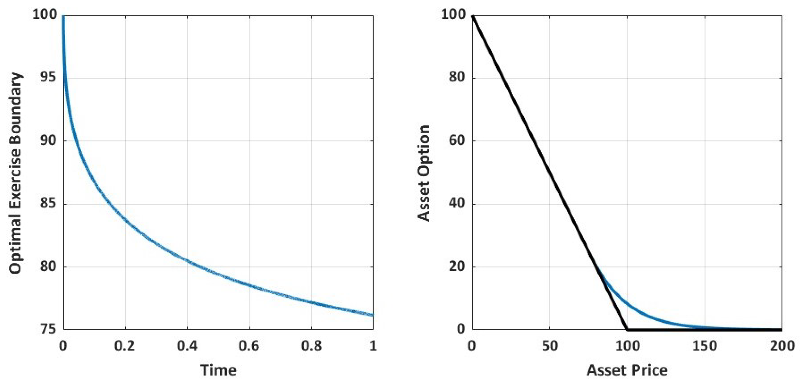
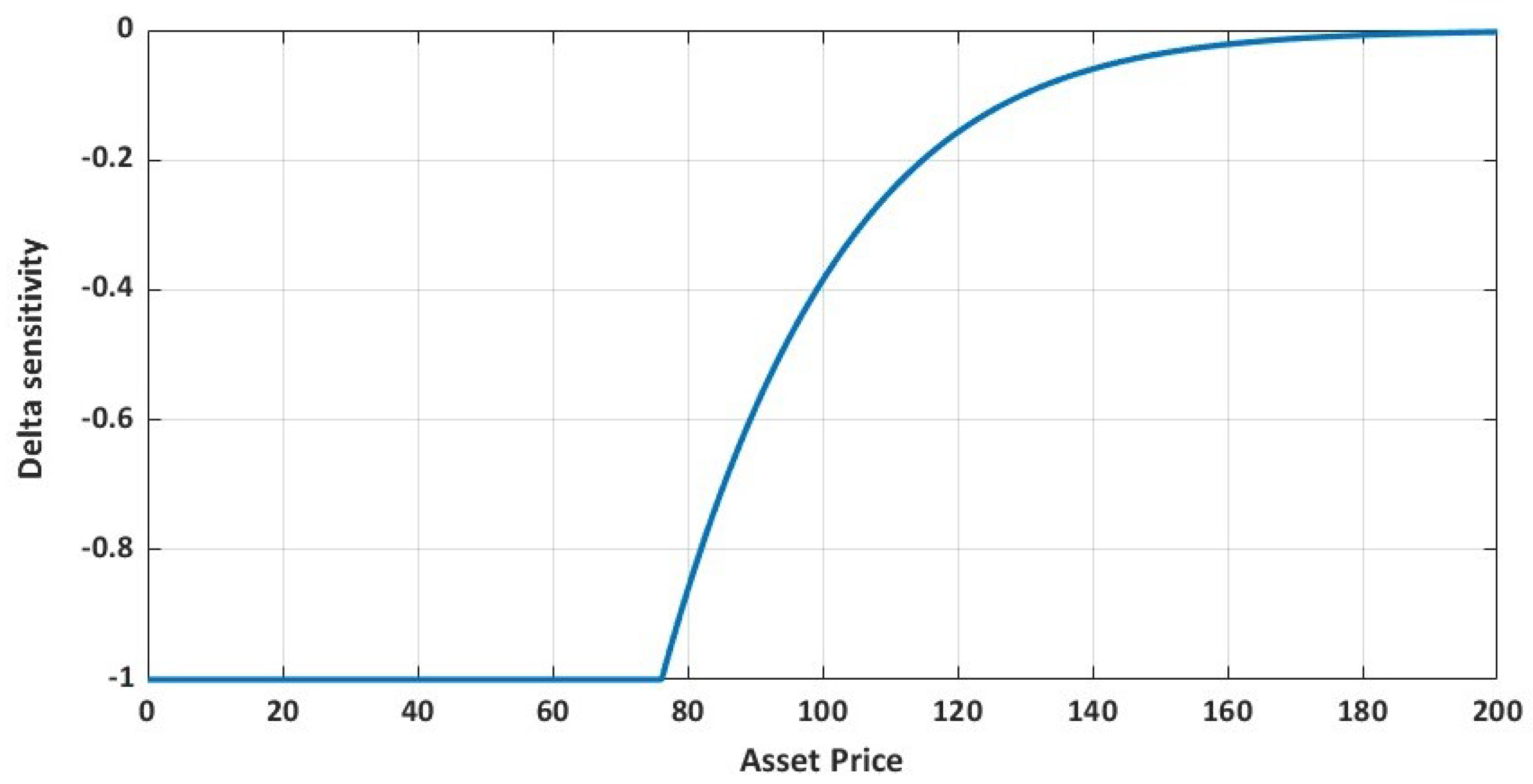
Note that the delta sensitivity is monotonically increasing and non-positive with
Moreover, the optimal exercise boundary is monotonically decreasing with
We refer the reader to the work of Kwok [
14], Musiela [
15], and Zhang et al. [
16] for details. Thus, we have
and
. Denote
Then, (
74) becomes
Note that
implying that
To ensure that
, we have to confirm
From (
76)–(
79), we have confirmed that
. Moreover, we see that
Since the first derivative of the optimal exercise boundary
is non-positive
, when
h is very small, we obtain
and
Next, we verify the right bound as given below
Simplifying further, we then obtain
Considering the non-positivity of the delta sensitivity coupled with an extrapolated Taylor series expansion, we can further obtain
Considering the left boundary value of the delta sensitivity and implied second derivative left boundary condition, we further obtain
Hence, with (
76) and a very small
h, we can obtain
Substituting to (
90), we then obtain
Note that
Let
Thus,
Here, we need to further obtain at least a reasonable upper bound for
in (
98) given as
To this end, we further simplify the denominator of (
99). Let
. If we derive Taylor series expansion around
, we further obtain the following:
If we consider (
100), (
101), left boundary values of the option value and delta sensitivity, and the implied left boundary value of the second derivative of the option value, we can further simplify the terms in
and
given in (
96) and (
97) as follows:
Note that
Substituting them into (
96) and (
97), we obtain
Furthermore, for a very small
h, we have
With further simplification of (
112), we obtain
Hence, we have
Here,
, where
is defined in (
78). For a very small
h, we further obtain
Thus, we have
and
To conclude our proof, we need to ensure that
which implies that
Hence, we conclude that if the assumption in (
119) holds, then


