Article

Higher-Order Blended Compact Difference Scheme on Nonuniform Grids for the 3D Steady Convection-Diffusion Equation

1
School of Mathematics and Computer Science, Ningxia Normal University, Guyuan 756000, China
2
School of Mathematics and Information Science, North Minzu University, Yinchuan 750021, China
3
School of Science, Dalian Minzu University, Dalian 116600, China
*
Author to whom correspondence should be addressed.
Axioms 2023, 12(7), 651; https://doi.org/10.3390/axioms12070651
Submission received: 22 May 2023 / Revised: 23 June 2023 / Accepted: 25 June 2023 / Published: 29 June 2023
(This article belongs to the Topic Numerical Methods for Partial Differential Equations)

Abstract

:
This paper proposes a higher-order blended compact difference (BCD) scheme on nonuniform grids for solving the three-dimensional (3D) convection–diffusion equation with variable coefficients. The BCD scheme has fifth- to sixth-order accuracy and considers the first and second derivatives of the unknown function as unknowns as well. Unlike other schemes that require grid transformation, the BCD scheme does not require any grid transformation and is simple and flexible in grid subdivisions. Concurrently, the corresponding high-order boundary schemes of the first and second derivatives have also been constructed. We tested the BCD scheme on three problems that involve convection-dominated and boundary-layer features. The numerical results show that the BCD scheme has good adaptability and high resolution on nonuniform grids. It outperforms the BCD scheme on uniform grids and the high-order compact scheme on nonuniform grids in the literature in terms of accuracy and resolution.

1. Introduction

In this work, we mainly study the following 3D convection-diffusion equation (CDE)
( a u x x + b u y y + c u z z ) + p u x + q u y + r u z = f   i n   Ω
where diffusive coefficients a , b , c are positive constants. The convection coefficients p , q , r , and the forcing term f , as well as the unknown function u , are functions of three variables x , y , and z and assumed to be sufficiently smooth on Ω = [ a 0 , a 1 ] × [ b 0 , b 1 ] × [ c 0 , c 1 ] . Ω is a cubic region in 3D space. A suitable Dirichlet condition is prescribed on the boundary Ω .
The CDE is widely concerned by many researchers since it can describe many physical phenomena, such as heat transfer, vorticity transport, mass, or concentration diffusion, etc., and it is also a simplified model of the incompressible Navier–Stokes equations used to describe fluid flow [1,2,3,4]. We also focused on this mode equation because, within the realm of computational fluid dynamics, there appears to be a predilection for the steady solutions of many evolutionary partial differential equations, as they are key to understanding complex fluid dynamics.
Because the analytic solution of CDE is very difficult to obtain in most cases, even impossible, the development of accurate, stable, and efficient numerical methods for solving it is of paramount importance. Over the past decades, high-order compact (HOC) finite difference methods have attracted more and more attention due to their many advantages, such as high accuracy, high resolution, small calculation amount, and relatively easy handling of boundary elements. A variety of specialized techniques have been developed based on HOC schemes to solve partial differential equations [5,6,7,8,9,10,11,12,13,14,15,16,17,18,19,20]. Generally, there are two classes of HOC schemes. One class is called explicit compact difference schemes [5,6,7,8,9,10,11,12,13], where all the derivatives are explicitly discretized by the nodal values of the objective function. That is, the difference equations do not include any derivatives. The other class is called implicit compact difference schemes [15,16,17,18,19,20], which treat the objective function and its derivatives together as unknown variables, and partial or all derivatives are involved in the calculation. The advantage of implicit compact difference schemes is that it is easy to obtain higher-accuracy compact difference schemes with high resolution. In 1998, Chu and Fan [17] introduced the combination compact difference (CCD) scheme, which is a classic implicit compact difference approach possessing sixth-order accuracy. Fourier analysis reveals that the CCD scheme outperforms other existing high-order compact and non-compact schemes in terms of spectral resolution. Unfortunately, the CCD scheme necessitates coupling all difference equations for the unknown function and its various derivatives, which must be solved in conjunction with the boundary scheme. This requirement inevitably leads to an extensive and intricate coefficient matrix, thereby increasing the complexity of algorithm design and programming. Recently, Ma and Ge [21] introduced a novel compact difference scheme, known as the BCD scheme, which combines the merits of explicit and implicit compact difference schemes for solving 3D CDEs. In comparison to the well-established CCD scheme [17], the BCD scheme not only attains high accuracy in both interior and boundary regions but also resolves the unknown function and its derivatives separately through an iterative procedure. Furthermore, the derivation process and algorithm design of the BCD scheme are straightforward and easily implemented.
The HOC schemes mentioned above are developed on uniform grids, which have good stability, high accuracy, and high resolution when solving smooth solution problems. However, when solving problems with large gradients and boundary layers, relatively poor calculation results are encountered if an insufficient number of grid points are allocated to regions with steep solution gradients [22,23]. To obtain higher-accuracy numerical results, more grid points, storage space, and computational effort are required. A more judicious strategy entails the utilization of nonuniform grids, wherein a greater number of grid points are allocated to regions with large gradients, while fewer grid points are assigned to regions with smaller gradients. In recent years, many compact difference schemes on nonuniform grids have been proposed to solve problems with large gradients or boundary layers [22,23,24,25,26]. Among them, the representative results based on the explicit compact difference schemes on nonuniform grids are as follows: Spotz and Carey [27] first proposed the HOC schemes for 1D and 2D CDEs without source terms on nonuniform grids in 1998. Afterward, Zhang et al. [28] developed a HOC scheme for the 3D CDE without source terms on nonuniform grids and performed direct numerical simulations for the problems with boundary layers. The methodology proposed in Refs. [27,28], known as coordinate transformation techniques; they convert nonuniform grids in the original physical domain into uniform grids within the computational domain. Subsequently, the numerical results in the computational domain are mapped back to the physical domain using inverse coordinate transformation. This approach allows the direct application of existing schemes constructed on uniform grids. However, a notable drawback of this method is that coordinate transformation often introduces additional terms into the transformed governing equation (e.g., cross-derivative terms), which inevitably increases the complexity of the equation [27,28]. Moreover, if the transformation is not explicitly known, it may necessitate the generation of solutions to certain differential equations, thereby introducing additional computations and potential errors. To avoid the above transformation, an alternative method was developed, which is to directly construct the difference scheme on nonuniform grids in the physical domain. The merit of this method lies in the ability to directly allocate a specific number of grids to boundary layers or regions with large gradients using straightforward grid-stretching functions, with the uniform grid configuration considered a special case. Kalita et al. [23] initially proposed a HOC scheme for the 2D CDE with variable coefficients on nonuniform grids and subsequently applied it to solve the 2D incompressible Navier–Stokes equations. Ge and Cao [24] developed a multigrid V-cycle algorithm based on the HOC scheme on nonuniform grids for solving the 2D CDE and used it to solve the classical lid-driven square cavity flow problem. Afterward, Ray and Kalita [29] proposed a third-order compact difference scheme for solving the 2D incompressible Navier–Stokes equations on nonuniform grids in polar coordinates and numerically simulated driven square cavity flow and flow around a cylinder. The representative results of the implicit compact difference schemes on nonuniform grids mainly include: Chu and Fan [30] developed a three-point fifth-order combined compact differences (CCD) on nonuniform grids. Shukla and Zhong [31] developed HOC schemes on nonuniform grids for first and second derivatives based on polynomial interpolation technology. Shukla et al. [32] extended the method in [31] to solve the stream function–vorticity formulation of the Navier–Stokes equations on nonuniform grids and numerically simulated-driven square cavity, flow around a cylinder, and heat convection problem in a square cavity. In 2013, Ge et al. [33] developed a transformation-free HOC scheme and the multigrid method on nonuniform grids for solving the 3D Poisson equation. Later, Shanab et al. [34] extended the work of Kalita et al. [23] to solve the 3D convection–diffusion equation with variable coefficients on nonuniform grids. It is a pity that the above scheme only has three- to four-order accuracy. In 2019, Ma and Ge [21] proposed a sixth-order BCD scheme on uniform grids to solve the 3D CDE with variable coefficients. As declared in the article, the BCD scheme on uniform grids is more suitable for dealing with smooth-solution problems, but it is not good at solving problems with boundary layers or local large gradients.
To the best of our knowledge, there have been no reported high-order BCD schemes on nonuniform grids for the 3D CDE with variable coefficients. The primary objective of this paper is to develop a transformation-free BCD method on nonuniform grids to solve the convection-dominated diffusion problems and the problems with boundary layers. The remainder of this article is structured as follows: Section 2 presents the high-order BCD scheme on nonuniform grids for the 3D CDE with variable coefficients. Subsequently, Section 3 provides a comparison of accuracy between the BCD scheme and other numerical methods. Lastly, Section 4 offers concluding remarks.

2. BCD Scheme on Nonuniform Grids

We discuss a cubic region Ω = [ a 0 , a 1 ] × [ b 0 , b 1 ] × [ c 0 , c 1 ] and perform discretization on a nonuniform 3D grid. Consequently, we partition the intervals [ a 0 , a 1 ] , [ b 0 , b 1 ] and [ c 0 , c 1 ] into sub-intervals, which are not necessarily of equal length, by the points a 0 = x 0 , x 1 , , x N x = a 1 , b 0 = y 0 , y 1 , , y N y = b 1 and c 0 = z 0 , z 1 , , z N z = c 1 . In x direction, allowing h x = ( a 1 a 0 ) / N x and defining h x θ r = x i + 1 x i , h x θ l = x i x i 1 , 1 i N x . Similarly, in y and z direction, allowing h y = ( b 1 b 0 ) / N y , h z = ( c 1 c 0 ) / N z , and defining h y θ f = y j + 1 y j , h y θ b = y j y j 1 ,   h z θ u = z k + 1 z k , h z θ d = z k z k 1 , 1 j N y , 1 k N z . For convenience, we also set α 1 = θ l θ r , β 1 = θ r + θ l , γ 1 = θ r θ l , α 2 = θ f θ b ,   β 2 = θ f + θ b , γ 2 = θ f θ b , α 3 = θ u θ d , β 3 = θ u + θ d , γ 3 = θ u θ d . If θ l = θ r = 1 ( θ f = θ b = 1 and θ d = θ u = 1 ), the result is a uniform grid.
We use the subscript notation u i , j , k = u ( x i , y j , z k ) and employ a local coordinate system where the cubic grids are labeled as in Figure 1. For convenience, we symbolize these derivatives by { u , u x , u x x , u y , u y y , u x y , u z , u z z , u y z }, respectively. As the presented BCD scheme involves independent calculations of first and second derivatives, achieving a fifth-order BCD scheme for the 3D CDE on nonuniform grids necessitates approximating all first and second derivatives to fifth-order accuracy. Therefore, we need to first derive the fifth-order scheme for the first and second derivatives, and then derive the fifth-order BCD scheme for the 3D CDE. Before deriving their formats above, we need to demonstrate an expression of a combination of fifth and sixth derivatives as an auxiliary formula.
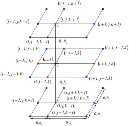
For the smooth function u ( x , y , z ) in Ω , Taylor series expansion at the point ( i + 1 , j , k ) is demonstrated as follows:
u i + 1 , j , k = u i , j , k + θ r h x ( u x ) i , j , k + ( θ r h x ) 2 2 ( u x x ) i , j , k + ( θ r h x ) 3 6 ( u x x x ) i , j , k + ( θ r h x ) 4 24 ( u x ( 4 ) ) i , j , k + ( θ r h x ) 5 120 ( u x ( 5 ) ) i , j , k + ( θ r h x ) 6 720 ( u x ( 6 ) ) i , j , k + O ( h x 7 )
Similarly, at point ( i 1 , j , k )
u i 1 , j , k = u i θ l h x ( u x ) i , j , k + ( θ l h x ) 2 2 ( u x x ) i , j , k ( θ l h x ) 3 6 ( u x x x ) i , j , k + ( θ l h x ) 4 24 ( u x ( 4 ) ) i , j , k ( θ l h x ) 5 120 ( u x ( 5 ) ) i , j , k + ( θ l h x ) 6 720 ( u x ( 6 ) ) i , j , k + O ( h x 7 )
Equation (2) multiplied by θ l 2 minus Equation (3) multiplied by θ r 2 , and rearranging it, results in
( u x ) i , j , k = δ x u i , j , k α 1 h x 2 6 ( u x x x ) i , j , k α 1 γ 1 h x 3 24 ( u x ( 4 ) ) i , j , k α 1 h x 4 120 ( γ 1 2 + α 1 ) ( u x ( 5 ) ) i , j , k α 1 γ 1 h x 5 720 ( γ 1 2 + 2 α 1 ) ( u x ( 6 ) ) i , j , k + O ( h x 6 )
Equation (2) multiplied by θ l plus Equation (3) multiplied by θ r , and rearranging it, results in
( u x x ) i , j , k = δ x 2 u i , j , k γ 1 h x 3 ( u x x x ) i , j , k h x 2 12 ( β 1 2 3 α 1 ) ( u x ( 4 ) ) i , j , k h x 3 60 γ 1 ( β 1 2 2 α 1 ) ( u x ( 5 ) ) i , j , k h x 4 360 ( γ 1 4 + 3 α 1 γ 1 2 + α 1 2 ) ( u x ( 6 ) ) i , j , k + O ( h x 5 )
where:
δ x u i , j , k = 1 α 1 β 1 h x ( θ l 2 u i + 1 , j , k + β 1 γ 1 u i , j , k θ r 2 u i 1 , j , k )
δ x 2 u i , j , k = 2 α 1 β 1 h x 2 ( θ l u i + 1 , j , k β 1 u i , j , k + θ r u i 1 , j , k )
In addition,
( u x x x ) i , j , k = δ x ( u x x ) i , j , k α 1 h x 2 6 ( u x ( 5 ) ) i , j , k α 1 γ 1 h x 3 24 ( u x ( 6 ) ) i , j , k + O ( h x 4 )
( u x ( 4 ) ) i , j , k = δ x 2 ( u x x ) i , j , k γ 1 h x 3 ( u x ( 5 ) ) i , j , k ( γ 1 2 + α 1 ) h x 2 12 ( u x ( 6 ) ) i , j , k + O ( h x 3 )
Here, we substitute Equations (8) and (9) into Equations (4) and (5), respectively. In addition, a rearrangement of the sequence of terms results in
( u x ) i , j , k = δ x u i , j , k α 1 h x 2 6 δ x ( u x x ) i , j , k α 1 γ 1 h x 3 24 δ x 2 ( u x x ) i , j , k   + h x 4 ( 7 α 1 2 + 2 α 1 γ 1 2 360 ) ( u x ( 5 ) ) i , j , k + h x 5 ( 11 α 1 2 γ 1 + 3 α 1 γ 1 3 1440 ) ( u x ( 6 ) ) i , j , k + O ( h x 6 )
( u x x ) i , j , k = δ x 2 ( u ) i , j , k γ 1 h x 3 δ x ( u x x ) i , j , k ( γ 1 2 + α 1 ) h x 2 12 δ x 2 ( u x x ) i , j , k   + ( 4 γ 1 3 + 18 α 1 γ 1 ) h x 3 360 ( u x ( 5 ) ) i , j , k + ( 28 α 1 γ 1 2 + 6 γ 1 4 + 6 α 1 2 ) h x 4 1440 ( u x ( 6 ) ) i , j , k + O ( h x 5 )
From Equations (10) and (11), we can obtain the following expressions of the fifth and sixth derivatives.
u x ( 5 ) = c ˜ 14 h x u x x c ˜ 12 u x + c ˜ 12 δ x u c ˜ 14 h x δ x 2 u + [ ( 2 c ˜ 14 γ 1 c ˜ 12 α 1 ) h x 2 / 6 ] δ x u x x + h x 3 [ c ˜ 14 ( γ 1 2 + α 1 ) / 12 c ˜ 12 ( γ 1 + α 1 ) / 24 ] δ x 2 u x x + O ( h x 2 )
u x ( 6 ) = c ˜ 11 u x c ˜ 13 h x u x x c ˜ 11 δ x u + c ˜ 13 h x δ x 2 u + [ ( c ˜ 11 α 1 2 c ˜ 13 γ 1 ) h x 2 / 6 ] δ x u x x + h x 3 [ c ˜ 11 α 1 γ 1 / 24 c ˜ 13 ( γ 1 2 + α 1 ) / 12 ] δ x 2 u x x + O ( h x 2 )
where:
c ˜ 11 = 1440 ( 4 γ 1 3 + 18 α 1 γ 1 ) h x 5 ( 10 α 1 3 γ 1 2 + 42 α 1 4 ) , c ˜ 12 = 360 ( 28 α 1 γ 1 2 + 6 γ 1 4 + 6 α 1 2 ) h x 4 ( 10 α 1 3 γ 1 2 + 42 α 1 4 ) c ˜ 13 = 1440 ( 7 α 1 2 + 2 α 1 γ 1 2 ) h x 5 ( 10 α 1 3 γ 1 2 + 42 α 1 4 ) , c ˜ 14 = 360 ( 11 α 1 2 γ 1 + 3 α 1 γ 1 3 ) h x 4 ( 10 α 1 3 γ 1 2 + 42 α 1 4 )
To derive the later formulas, we show the linear combination of the fifth and sixth derivatives from Equation (2) and (3) as follows:
T 11 u x ( 5 ) + T 12 u x ( 6 ) = ( T 11 c ˜ 12 T 12 c ˜ 11 ) δ x u + ( T 12 c ˜ 13 h x T 11 c ˜ 14 h x ) δ x 2 u + ( T 12 c ˜ 11 T 11 c ˜ 12 ) u x [ T 11 h x 2 ( 2 c ˜ 14 γ 1 c ˜ 12 α 1 ) / 6 + T 12 h x 2 ( c ˜ 11 α 1 2 c ˜ 13 γ 1 ) / 6 ] δ x u x x + ( T 11 c ˜ 14 h x T 12 c ˜ 13 h x ) u x x { T 11 h x 3 ( 2 c ˜ 14 ( α 1 + γ 1 2 ) c ˜ 12 α 1 γ 1 ) / 24 + T 12 h x 3 [ c ˜ 11 α 1 γ 1 2 c ˜ 13 ( α 1 + γ 1 2 ) ] / 24 } δ x 2 u x x
In addition, we define
d ˜ 11 = T 11 c ˜ 12 T 12 c ˜ 11 , d ˜ 16 = d ˜ 11 , d ˜ 12 = T 12 c ˜ 13 h x T 11 c ˜ 14 h x , d ˜ 15 = d ˜ 12 d ˜ 13 = [ T 11 h x 3 ( 2 c ˜ 14 ( α 1 + γ 1 2 ) c ˜ 12 α 1 γ 1 ) + T 12 h x 3 ( c ˜ 11 α 1 γ 1 2 c ˜ 13 ( α 1 + γ 1 2 ) ) ] / 24 d ˜ 14 = [ T 11 h x 2 ( 2 c ˜ 14 γ 1 c ˜ 12 α 1 ) + T 12 h x 2 ( c ˜ 11 α 1 2 c ˜ 13 γ 1 ) ] / 6
Then, the result is
T 11 u x ( 5 ) + T 12 u x ( 6 ) = d ˜ 11 δ x u + d ˜ 12 δ x 2 u + d ˜ 13 δ x 2 u x x + d ˜ 14 δ x u x x + d ˜ 15 u x x + d ˜ 16 u x

2.1. The Fifth-Order Compact Schemes for the First Derivatives { u x , u y , u z }

Since
( u x ) i , j , k = δ x ( u ) i , j , k + ( α 1 γ 1 2 + 6 α 1 2 ) h x 4 1080 ( u x ( 5 ) ) i , j , k + ( α 1 γ 1 3 + 7 α 1 2 γ 1 ) h x 5 4320 ( u x ( 6 ) ) i , j , k + α 1 γ 1 h x 3 72 δ x 2 ( u x x ) i , j , k α 1 h x 2 6 δ x 2 ( u x ) i , j , k + O ( h x 6 )
Substituting Equation (17) into Equation (18), we obtain
( u x ) i , j , k = 1 + d ˜ 11 1 d ˜ 16 δ x u i , j , k α 1 h x 2 6 ( 1 + d ˜ 11 ) δ x 2 ( u x ) i , j , k d ˜ 15 1 + d ˜ 11 ( u x x δ x 2 u ) i , j , k + α 1 γ 1 h x 3 + 72 d ˜ 13 72 ( 1 + d ˜ 11 ) δ x 2 ( u x x ) i , j , k d ˜ 14 1 + d ˜ 11 δ x ( u x x ) i , j , k + ( h x 6 )
Substituting Equations (6) and (7) into Equation (18), we obtain the fifth-to-sixth-order scheme for the first derivative u x on nonuniform grids.
θ l 3 β 1 ( 1 + d ˜ 11 ) ( u x ) i + 1 , j , k + 2 + 3 d ˜ 11 3 ( 1 + d ˜ 11 ) ( u x ) i , j , k + θ r 3 β 1 ( 1 + d ˜ 11 ) ( u x ) i 1 , j , k = [ θ l 2 ( 1 + d ˜ 11 ) α 1 β 1 h x ( 1 d ˜ 16 ) + 2 θ l d ˜ 15 α 1 β 1 h x 2 ( 1 + d ˜ 11 ) ] u i + 1 , j , k + [ γ 1 ( 1 + d ˜ 11 ) α 1 h x ( 1 d ˜ 16 ) 2 d ˜ 15 α 1 h x 2 ( 1 + d ˜ 11 ) ] u i , j , k [ θ r 2 ( 1 + d ˜ 11 ) α 1 β 1 h x ( 1 d ˜ 16 ) 2 θ r d ˜ 15 α 1 β 1 h x 2 ( 1 + d ˜ 11 ) ] u i 1 , j , k + [ θ l ( α 1 γ 1 h x 3 + 72 d ˜ 13 ) 36 α 1 β 1 h x 2 ( 1 + d ˜ 11 ) θ l 2 d ˜ 14 α 1 β 1 h x ( 1 + d ˜ 11 ) ] ( u x x ) i + 1 , j , k [ γ 1 d ˜ 14 + α 1 h x d ˜ 15 α 1 h x ( 1 + d ˜ 11 ) + α 1 γ 1 h x 3 + 72 d ˜ 13 36 α 1 h x 2 ( 1 + d ˜ 11 ) ] ( u x x ) i , j , k + [ θ r 2 d ˜ 14 α 1 β 1 h x ( 1 + d ˜ 11 ) + θ r ( α 1 γ 1 h x 3 + 72 d ˜ 13 ) 36 α 1 β 1 h x 2 ( 1 + d ˜ 11 ) ] ( u x x ) i 1 , j , k
Similarly, we also obtain the fifth-to-sixth-order schemes for the first derivatives u y and u z on nonuniform grids, as follows:
θ b 3 β 2 ( 1 + d ˜ 21 ) ( u y ) i , j + 1 , k + 2 + 3 d ˜ 21 3 ( 1 + d ˜ 21 ) ( u y ) i , j , k + θ f 3 β 2 ( 1 + d ˜ 21 ) ( u y ) i , j 1 , k = [ θ b 2 ( 1 + d ˜ 21 ) α 2 β 2 h y ( 1 d ˜ 26 ) + 2 θ b d ˜ 25 α 2 β 2 h y 2 ( 1 + d ˜ 21 ) ] u i , j + 1 , k + [ γ 2 ( 1 + d ˜ 21 ) α 2 h y ( 1 d ˜ 26 ) 2 d ˜ 25 α 2 h y 2 ( 1 + d ˜ 21 ) ] u i , j , k [ θ f 2 ( 1 + d ˜ 21 ) α 2 β 2 h y ( 1 d ˜ 26 ) 2 θ f d ˜ 25 α 2 β 2 h y 2 ( 1 + d ˜ 21 ) ] u i , j 1 , k + [ θ b ( α 2 γ 2 h y 3 + 72 d ˜ 23 ) 36 α 2 β 2 h y 2 ( 1 + d ˜ 21 ) θ b 2 d ˜ 24 α 2 β 2 h y ( 1 + d ˜ 21 ) ] ( u y y ) i , j + 1 , k [ γ 2 d ˜ 24 + α 2 h y d ˜ 25 α 2 h y ( 1 + d ˜ 21 ) + α 2 γ 2 h y 3 + 72 d ˜ 23 36 α 2 h y 2 ( 1 + d ˜ 21 ) ] ( u y y ) i , j , k + [ θ f 2 d ˜ 24 α 2 β 2 h y ( 1 + d ˜ 21 ) + θ f ( α 1 γ 1 h y 3 + 72 d ˜ 23 ) 36 α 2 β 2 h y 2 ( 1 + d ˜ 21 ) ] ( u y y ) i , j 1 , k
where:
δ y u i , j , k = ( θ b 2 u i , j + 1 , k + β 2 γ 2 u i , j , k θ f 2 u i , j 1 , k ) / α 2 β 2 h y
δ y 2 u i , j , k = 2 ( θ b u i , j + 1 , k β 2 u i , j , k + θ f u i , j 1 , k ) / α 2 β 2 h y 2
δ z u i , j , k = ( θ d 2 u i , j , k + 1 + β 3 γ 3 u i , j , k θ u 2 u i , j , k 1 ) / α 3 β 3 h z
δ z 2 u i , j , k = 2 ( θ d u i , j , k + 1 β 2 u i , j , k + θ u u i , j , k 1 ) / α 3 β 3 h z 2
d ˜ 21 = T 21 c ˜ 22 T 22 c ˜ 21 , d ˜ 22 = T 22 c ˜ 23 h y T 21 c ˜ 24 h y , d ˜ 25 = d ˜ 22 , d ˜ 23 = [ T 21 h y 3 ( 2 c ˜ 24 ( α 2 + γ 2 2 ) c ˜ 22 α 2 γ 2 ) + T 22 h y 3 ( c ˜ 21 α 2 γ 2 2 c ˜ 23 ( α 2 + γ 2 2 ) ) ] / 24 d ˜ 24 = T 21 h y 2 ( 2 c ˜ 24 γ 2 c ˜ 22 α 2 ) / 6 + T 22 h y 2 ( c ˜ 21 α 2 2 c ˜ 23 γ 2 ) / 6 , d ˜ 26 = d ˜ 21
c ˜ 21 = 1440 ( 4 γ 2 3 + 18 α 2 γ 2 ) h y 5 ( 10 α 2 3 γ 2 2 + 42 α 2 4 ) , c ˜ 22 = 360 ( 28 α 2 γ 2 2 + 6 γ 2 4 + 6 α 2 2 ) h y 4 ( 10 α 2 3 γ 2 2 + 42 α 2 4 ) c ˜ 23 = 1440 ( 7 α 2 2 + 2 α 2 γ 2 2 ) h y 5 ( 10 α 2 3 γ 2 2 + 42 α 2 4 ) , c ˜ 24 = 360 ( 11 α 2 2 γ 2 + 3 α 2 γ 2 3 ) h y 4 ( 10 α 2 3 γ 2 2 + 42 α 2 4 )
T 21 = ( 6 α 2 2 + α 2 γ 2 2 ) h y 4 / 1080 , T 22 = ( 7 α 2 2 γ 2 + α 2 γ 2 3 ) h y 5 / 4320 d ˜ 31 = T 31 c ˜ 32 T 32 c ˜ 31 , d ˜ 32 = T 32 c ˜ 33 h z T 31 c ˜ 34 h z , d ˜ 35 = d ˜ 32 , d ˜ 33 = [ T 31 h z 3 ( 2 c ˜ 34 ( α 3 + γ 3 2 ) c ˜ 32 α 3 γ 3 ) + T 32 h z 3 ( c ˜ 31 α 3 γ 3 2 c ˜ 33 ( α 3 + γ 3 2 ) ) ] / 24 ,
d ˜ 34 = T 31 h z 2 ( 2 c ˜ 34 γ 2 c ˜ 32 α 3 ) / 6 + T 32 h z 2 ( c ˜ 31 α 3 2 c ˜ 33 γ 3 ) / 6 ,   d ˜ 36 = d ˜ 61 ,
c ˜ 31 = 1440 ( 4 γ 3 3 + 18 α 3 γ 3 ) h z 5 ( 10 α 3 3 γ 3 2 + 42 α 3 4 ) , c ˜ 32 = 360 ( 28 α 3 γ 3 2 + 6 γ 3 4 + 6 α 3 2 ) h z 4 ( 10 α 3 3 γ 3 2 + 42 α 3 4 ) , c ˜ 33 = 1440 ( 7 α 3 2 + 2 α 3 γ 3 2 ) h z 5 ( 10 α 3 3 γ 3 2 + 42 α 3 4 ) , c ˜ 34 = 360 ( 11 α 3 2 γ 3 + 3 α 3 γ 3 3 ) h z 4 ( 10 α 3 3 γ 3 2 + 42 α 3 4 ) ,
T 31 = ( 6 α 3 2 + α 3 γ 3 2 ) h z 4 / 1080 , T 32 = ( 7 α 3 2 γ 3 + α 3 γ 3 3 ) h z 5 / 4320 .

2.2. The Fifth-Order Compact Schemes for the Second Derivatives { u x x , u y y , u z z }

It is noted that
u x x = 2 α 1 α 1 γ 1 2 δ x 2 u ( γ 1 2 + α 1 ) α 1 γ 1 2 δ x u x 2 α 1 γ 1 h x 3 ( α 1 γ 1 2 ) δ x u x x + h x 3 α 1 γ 1 ( 31 α 1 + 3 γ 1 2 ) 360 ( α 1 γ 1 2 ) u x ( 5 ) + h x 4 α 1 ( 10 α 1 γ 1 2 + γ 1 4 + α 1 2 ) 360 ( α 1 γ 1 2 ) u x ( 6 ) + O ( h x 5 )
Substituting Equation (15) into Equation (33), the fifth-order compact scheme for the second derivative u x x on nonuniform grids is obtained as follows:
+ ( E ˜ 12 θ l 2 α 1 β 1 h x 2 E ˜ 13 θ l α 1 β 1 h x 2 ) ( u x x ) i + 1 , j , k + ( 1 γ 1 E ˜ 12 α 1 h x 2 E ˜ 13 α 1 h x 2 ) ( u x x ) i , j , k + ( E ˜ 12 θ r 2 α 1 β 1 h x 2 E ˜ 13 θ r α 1 β 1 h x 2 ) ( u x x ) i 1 , j , k = ( 2 E ˜ 11 θ l α 1 β 1 h x 2 E ˜ 14 θ l 2 α 1 β 1 h x ) u i + 1 , j , k ( 2 E ˜ 11 α 1 h x 2 + E ˜ 14 γ 1 α 1 h x ) u i , j , k + ( 2 E ˜ 11 θ r α 1 β 1 h x 2 + E ˜ 14 θ r 2 α 1 β 1 h x ) u i 1 , j , k + E ˜ 16 θ l 2 α 1 β 1 h x ( u x ) i + 1 , j , k + ( E ˜ 16 γ 1 α 1 h x + E ˜ 14 ) ( u x ) i , j , k ( E ˜ 16 θ r 2 α 1 β 1 h x ) ( u x ) i 1 , j , k
Similarly, the fifth-order schemes for the second derivatives { u y y , u z z } on nonuniform grids are also obtained as follows:
( h y E ˜ 22 θ b 2 + 2 E ˜ 23 θ b α 2 β 2 h y 2 ) ( u y y ) i , j + 1 , k + ( 1 γ 2 E ˜ 22 α 2 h y 2 E ˜ 23 α 2 h y 2 ) ( u y y ) i , j , k + ( E ˜ 22 θ f 2 α 2 β 2 h y 2 E ˜ 23 θ f α 2 β 2 h y 2 ) ( u y y ) i , j 1 , k = ( 2 E ˜ 21 θ b α 2 β 2 h y 2 E ˜ 24 θ b 2 α 2 β 2 h y ) u i , j + 1 , k ( 2 E ˜ 21 α 2 h y 2 + E ˜ 24 γ 2 α 2 h y ) u i , j , k + ( 2 E ˜ 21 θ f α 2 β 2 h y 2 + E ˜ 24 θ f 2 α 2 β 2 h y ) u i , j 1 , k + E ˜ 26 θ b 2 α 2 β 2 h y ( u y ) i , j + 1 , k + ( E ˜ 26 γ 2 α 2 h y + E ˜ 24 ) ( u y ) i , j , k E ˜ 26 θ f 2 α 2 β 2 h y ( u y ) i , j 1 , k
( E ˜ 32 δ d 2 α 3 β 3 h z 2 E ˜ 33 δ d α 3 β 3 h z 2 ) ( u z z ) i , j , k + 1 + ( 1 γ 3 E ˜ 32 α 3 h z 2 E ˜ 33 α 3 h z 2 ) ( u z z ) i , j , k + ( E ˜ 32 θ u 2 α 3 β 3 h z 2 E ˜ 33 θ u α 3 β 3 h z 2 ) ( u z z ) i , j , k 1 = ( 2 E ˜ 31 θ d α 3 β 3 h z 2 E ˜ 34 θ d 2 α 3 β 3 h z ) u i , j , k + 1 ( 2 E ˜ 31 α 3 h z 2 + E ˜ 34 γ 1 α 3 h z ) u i , j , k + ( 2 E ˜ 31 θ u α 3 β 3 h z 2 + E ˜ 34 θ u 2 α 3 β 3 h z ) u i , j , k 1 + E ˜ 36 θ d 2 α 3 β 3 h z ( u z ) i , j , k + 1 + ( E ˜ 36 γ 3 α 3 h z + E ˜ 34 ) ( u z ) i , j , k ( E ˜ 36 θ u 2 α 3 β 3 h z ) ( u z ) i , j , k 1
where:
E ˜ 11 = d ˜ 12 α 1 d ˜ 12 γ 1 2 + 2 α 1 ( α 1 γ 1 2 ) ( 1 d ˜ 15 ) , E ˜ 12 = 3 d ˜ 14 ( α 1 γ 1 2 ) 2 h x α 1 γ 1 3 ( α 1 γ 1 2 ) ( 1 d ˜ 15 ) , E ˜ 13 = d ˜ 13 1 d ˜ 15 , E ˜ 14 = d ˜ 16 1 d ˜ 15 , E ˜ 15 = d ˜ 11 1 d ˜ 15 , E ˜ 16 = α 1 + γ 1 2 ( α 1 γ 1 2 ) ( 1 d ˜ 15 )
E ˜ 21 = d ˜ 22 α 2 d ˜ 22 γ 2 2 + 2 α 2 ( α 2 γ 2 2 ) ( 1 d ˜ 25 ) , E ˜ 22 = 3 d ˜ 24 ( α 2 γ 2 2 ) 2 h y α 2 γ 2 3 ( α 2 γ 2 2 ) ( 1 d ˜ 25 ) , E ˜ 23 = d ˜ 23 1 d ˜ 25 , E ˜ 24 = d ˜ 26 1 d ˜ 25 , E ˜ 25 = d ˜ 21 1 d ˜ 25 , E 26 = α 2 + γ 2 2 ( α 2 γ 2 2 ) ( 1 d ˜ 25 )
E ˜ 31 = d ˜ 32 α 3 d ˜ 32 γ 3 2 + 2 α 3 ( α 3 γ 3 2 ) ( 1 d ˜ 35 ) , E ˜ 32 = 3 d ˜ 34 ( α 3 γ 3 2 ) 2 h z α 3 γ 3 3 ( α 3 γ 3 2 ) ( 1 d ˜ 35 ) , E ˜ 33 = d ˜ 33 1 d ˜ 35 , E ˜ 34 = d ˜ 36 1 d ˜ 35 , E ˜ 35 = d ˜ 31 1 d ˜ 35 , E ˜ 36 = α 3 + γ 3 2 ( α 3 γ 3 2 ) ( 1 d ˜ 35 ) .

2.3. BCD Schemes of the 3D CDE on Nonuniform Grids

By Taylor series expansion, we obtain
u x = δ x u α 1 h x 2 6 u x x x α 1 γ 1 h x 3 24 u x ( 4 ) α 1 h x 4 120 ( γ 1 2 + α 1 ) u x ( 5 ) α 1 γ 1 h x 5 720 ( γ 1 2 + 2 α 1 ) u x ( 6 ) + O ( h x 6 )
u y = δ y u α 2 h y 2 6 u y y y α 2 γ 2 h y 3 24 u y ( 4 ) α 2 h y 4 120 ( γ 2 2 + α 2 ) u y ( 5 ) α 2 γ 2 h y 5 720 ( γ 2 2 + 2 α 2 ) u y ( 6 ) + O ( h y 6 )
u z = δ z u α 3 h z 2 6 u z z z α 3 γ 3 h z 3 24 u z ( 4 ) α 3 h z 4 120 ( γ 3 2 + α 3 ) u z ( 5 ) α 3 γ 3 h z 5 720 ( γ 3 2 + 2 α 3 ) u z ( 6 ) + O ( h z 6 )
Substituting Equations (40)–(42) into Equation (1), we obtain
a u x x b u y y c u z z + p δ x u + q δ y u + r δ z u p α 1 h x 2 6 u x x x p α 1 γ 1 h x 3 24 u x ( 4 ) p α 1 h x 4 120 ( γ 1 2 + α 1 ) u x ( 5 ) p α 1 γ 1 h x 5 720 ( γ 1 2 + 2 α 1 ) u x ( 6 ) q α 2 h y 2 6 u y y y q α 2 γ 2 h y 3 24 u y ( 4 ) q α 2 h y 4 120 ( γ 2 2 + α 2 ) u y ( 5 ) q α 2 γ 2 h y 5 720 ( γ 2 2 + 2 α 2 ) u y ( 6 ) r α 3 h z 2 6 u z z z r α 3 γ 3 h z 3 24 u z ( 4 ) r α 3 h z 4 120 ( γ 3 2 + α 3 ) u z ( 5 ) r α 3 γ 3 h z 5 720 ( γ 3 2 + 2 α 3 ) u z ( 6 ) + O ( h x 6 + h y 6 + h z 6 ) = f ( x , y , z )
With the differentiating Equation (1) concerning x , y , and z , we obtain
u x x x = 1 a ( b u y y x c u z z x + p u x x + p x u x + q u y x + q x u y + r u z x + r x u z f x )
u y y y = 1 b ( a u x x y c u z z y + p u x y + p y u x + q u y y + q y u y + r u z y + r y u z f y )
u z z z = 1 c ( a u x x z b u y y z + p u x z + p z u x + q u y z + q z u y + r u z z + r z u z f z )
Substituting Equations (44)–(46) into Equation (43), we obtain
( a p 2 α 1 h x 2 6 a ) u x x + ( b q 2 α 2 h y 2 6 b ) u y y + ( c r 2 α 3 h z 2 6 c ) u z z + p δ x u + q δ y u + r δ z u + ( p p x α 1 h x 2 6 a q p y α 2 h y 2 6 b r p z α 3 h z 2 6 c ) u x + ( p q x α 1 h x 2 6 a q q y α 2 h y 2 6 b r q z α 3 h z 2 6 c ) u x + ( p r x α 1 h x 2 6 a q r y α 2 h y 2 6 b r r z α 3 h z 2 6 c ) u z + ( p q α 1 h x 2 6 a q p α 2 h y 2 6 b ) u x y + ( q r α 2 h y 2 6 b q r α 3 h z 2 6 c ) u y z + ( p r α 1 h x 2 6 a r p α 3 h z 2 6 c ) u z x + b p α 1 h x 2 6 a u y y x + c p α 1 h x 2 6 a u z z x + a q α 2 h y 2 6 b u x x y + c q α 2 h y 2 6 b u z z y + a r α 3 h z 2 6 c u x x z + b r α 3 h z 2 6 c u y y z p α 1 γ 1 h x 3 24 u x ( 4 ) p α 1 h x 4 120 ( γ 1 2 + α 1 ) u x ( 5 ) p α 1 γ 1 h x 5 720 ( γ 1 2 + 2 α 1 ) u x ( 6 ) q α 2 γ 2 h y 3 24 u y ( 4 ) q α 2 h y 4 120 ( γ 2 2 + α 2 ) u y ( 5 ) q α 2 γ 2 h y 5 720 ( γ 2 2 + 2 α 2 ) u y ( 6 ) r α 3 γ 3 h z 3 24 u z ( 4 ) r α 3 h z 4 120 ( γ 3 2 + α 3 ) u z ( 5 ) r α 3 γ 3 h z 5 720 ( γ 3 2 + 2 α 3 ) u z ( 6 ) + O ( h x 6 + h y 6 + h z 6 ) = f p α 1 h x 2 6 a f x q α 2 h y 2 6 b f y r α 3 h z 2 6 c f z
In addition, after rearranging the sequence of terms, we obtain
B 1 u x x + B 2 u y y + B 3 u z z + p δ x u + q δ y u + r δ z u + B 4 u x + B 5 u y + B 6 u z + B 7 u x y + B 8 u y z + B 9 u z x + B 10 u y y x + B 11 u z z x + B 12 u x x y + B 13 u z z y + B 14 u x x z + B 15 u y y z + B 16 δ x 2 u x x + B 17 δ y 2 u y y + B 18 δ z 2 u z z + W 1 + W 2 + W 3 + O ( h x 6 + h y 6 + h z 6 ) = F
where:
B 1 = a α 1 h x 2 p 2 6 a , B 2 = b α 2 h y 2 q 2 6 b , B 3 = c α 3 h z 2 r 2 6 c , B 4 = α 1 h x 2 p p x 6 a α 2 h y 2 q p y 6 b α 3 h z 2 r p z 6 c , B 5 = α 1 h x 2 p q x 6 a α 2 h y 2 q q y 6 b α 3 h z 2 r q z 6 c , B 6 = α 1 h x 2 p r x 6 a α 2 h y 2 q r y 6 b α 3 h z 2 r r z 6 c , B 7 = α 1 h x 2 p q 6 a α 2 h y 2 q p 6 b , B 8 = α 2 h y 2 q r 6 b α 3 h z 2 r q 6 c , B 9 = α 1 h x 2 p r 6 a α 3 h z 2 r p 6 c , B 10 = α 1 h x 2 p b 6 a , B 11 = α 1 h x 2 p c 6 a , B 12 = α 2 h y 2 q a 6 b , B 13 = α 2 h y 2 q c 6 b , B 14 = α 3 h z 2 r a 6 c , B 15 = α 3 h z 2 r b 6 c , B 16 = p α 1 γ 1 h x 3 24 , B 17 = q α 2 γ 2 h y 3 24 , B 18 = r α 3 γ 3 h z 3 24 , F = f h x 2 p α 1 6 a f x h y 2 q α 2 6 b f y h z 2 r α 3 6 c f z W 1 = p h x 4 ( 2 α 1 γ 1 2 3 α 1 2 ) 360 u x ( 5 ) + p h x 5 ( 3 α 1 γ 1 3 + α 1 2 γ 1 ) 1440 u x ( 6 ) W 2 = q h y 4 ( 2 α 2 γ 2 2 3 α 2 2 ) 360 u y ( 5 ) + q h y 5 ( 3 α 2 γ 2 3 + α 2 2 γ 2 ) 1440 u y ( 6 ) W 3 = r h z 4 ( 2 α 3 γ 3 2 3 α 3 2 ) 360 u z ( 5 ) + r h z 5 ( 3 α 3 γ 3 3 + α 3 2 γ 3 ) 1440 u z ( 6 )
To obtain a fifth-order compact formulation for Equation (48), we consider the following approximations.
u x x = 2 α 1 α 1 γ 1 2 δ x 2 u ( γ 1 2 + α 1 ) α 1 γ 1 2 δ x u x 2 α 1 γ 1 h x 3 ( α 1 γ 1 2 ) δ x u x x + h x 3 α 1 γ 1 ( 31 α 1 + 3 γ 1 2 ) 360 ( α 1 γ 1 2 ) u x ( 5 ) + h x 4 α 1 ( 10 α 1 γ 1 2 + γ 1 4 + α 1 2 ) 360 ( α 1 γ 1 2 ) u x ( 6 ) + O ( h x 5 ) u y y = 2 α 2 α 2 γ 2 2 δ y 2 u ( γ 2 2 + α 2 ) α 2 γ 2 2 δ y u y 2 α 2 γ 2 h y 3 ( α 2 γ 2 2 ) δ y u y y + h y 3 α 2 γ 2 ( 31 α 2 + 3 γ 2 2 ) 360 ( α 2 γ 2 2 ) u y ( 5 ) + h y 4 α 2 ( 10 α 2 γ 2 2 + γ 2 4 + α 2 2 ) 360 ( α 2 γ 2 2 ) u y ( 6 ) + O ( h y 5 ) u z z = 2 α 3 α 3 γ 3 2 δ z 2 u ( γ 3 2 + α 3 ) α 3 γ 3 2 δ z u z 2 α 3 γ 3 h z 3 ( α 3 γ 3 2 ) δ z u z z + h x 3 α 1 γ 3 ( 31 α 1 + 3 γ 3 2 ) 360 ( α 3 γ 3 2 ) u z ( 5 ) + h z 4 α 3 ( 10 α 3 γ 3 2 + γ 3 4 + α 3 2 ) 360 ( α 3 γ 3 2 ) u z ( 6 ) + O ( h z 5 )
u x y = δ x u y + δ y u x δ x δ y u + O ( h x 3 + h y 3 + h y h x 2 + h x h y 2 ) u y z = δ z u y + δ y u z δ z δ y u + O ( h z 3 + h y 3 + h y h z 2 + h z h y 2 ) u x z = δ x u z + δ z u x δ x δ z u + O ( h x 3 + h z 3 + h z h x 2 + h x h z 2 ) u x x y = δ x 2 u y + δ y u x x δ y δ x 2 u + O ( h x 3 + h y 3 + h x 2 h y ) u y y x = δ y 2 u x + δ x u y y δ x δ y 2 u + O ( h x 3 + h y 3 + h y 2 h x ) u x x z = δ x 2 u z + δ z u x x δ z δ x 2 u + O ( h x 3 + h z 3 + h x 2 h z ) u z z x = δ z 2 u x + δ x u z z δ x δ z 2 u + O ( h x 3 + h z 3 + h z 2 h x ) u y y z = δ y 2 u z + δ z u y y δ z δ y 2 u + O ( h z 3 + h y 3 + h y 2 h z ) u z z y = δ z 2 u y + δ y u z z δ y δ z 2 u + O ( h z 3 + h y 3 + h z 2 h y )
Substituting Equations (50) and (51) into Equation (48), and using the conclusion of Equation (15) again, we obtain
( 2 α 1 B 1 α 1 γ 1 2 + d ˜ 12 ) δ x 2 u + ( p + d ˜ 11 ) δ x u + ( 2 α 2 B 2 α 2 γ 2 2 + d ˜ 22 ) δ y 2 u + ( q + d ˜ 21 ) δ y u + ( 2 B 3 α 3 α 3 γ 3 2 + d ˜ 32 ) δ z 2 u + ( r + d ˜ 31 ) δ z u B 7 δ x δ y u B 8 δ z δ y u B 9 δ x δ z u B 10 δ x δ y 2 u B 11 δ x δ z 2 u B 12 δ y δ x 2 u B 13 δ y δ z 2 u B 14 δ z δ x 2 u B 15 δ z δ y 2 u B 1 ( γ 1 2 + α 1 ) α 1 γ 1 2 δ x u x + ( B 4 + d ˜ 16 ) u x + B 7 δ y u x + B 9 δ z u x + B 10 δ y 2 u x + B 11 δ z 2 u x + ( d ˜ 14 2 B 1 α 1 γ 1 h x 3 ( α 1 γ 1 2 ) ) δ x u x x + B 12 δ y u x x + B 14 δ z u x x + B 16 δ x 2 u x x + d ˜ 13 δ x 2 u x x + d ˜ 15 u x x
B 2 ( γ 2 2 + α 2 ) α 2 γ 2 2 δ y u y + ( B 5 + d ˜ 26 ) u y + B 7 δ x u y + B 8 δ z u y + B 12 δ x 2 u y + B 13 δ z 2 u y + ( d ˜ 24 2 B 2 α 2 γ 2 h y 3 ( α 2 γ 2 2 ) ) δ y u y y + B 17 δ y 2 u y y + B 15 δ z u y y + B 10 δ x u y y + d ˜ 23 δ y 2 u y y + d ˜ 25 u y y B 3 ( γ 3 2 + α 3 ) α 3 γ 3 2 δ z u z + ( B 6 + d ˜ 36 ) u z + B 8 δ y u z + B 9 δ x u z + B 14 δ x 2 u z + B 15 δ y 2 u z + ( d ˜ 34 2 B 3 α 3 γ 3 h z 3 ( α 3 γ 3 2 ) ) δ z u z z + B 18 δ z 2 u z z + B 13 δ y u z z + B 11 δ x u z z + d ˜ 33 δ z 2 u z z + d ˜ 35 u z z + O ( h x 5 + h y 5 + h z 5 + h x 2 h y 3 + h x 2 h z 3 + h y 2 h x 3 + h y 2 h z 3 + h z 2 h x 3 + h z 2 h y 3 ) = F
where, the differential operators { δ x δ y , δ x 2 δ y , δ y 2 δ x , δ y δ z , δ y 2 δ z , δ z 2 δ y , δ x δ z , δ x 2 δ z , δ z 2 δ x } can be referred to Appendix A. Neglecting the truncation error terms, the 19-point fifth-order BCD scheme on nonuniform for the 3D CDE is demonstrated as follows:
C ˜ 0 u i , j , k + C ˜ 1 u i + 1 , j , k + C ˜ 2 u i , j + 1 , k + C ˜ 3 u i 1 , j , k + C ˜ 4 u i , j 1 , k + C ˜ 5 u i , j , k + 1 + C ˜ 6 u i , j , k 1 + C ˜ 7 u i + 1 , j + 1 , k + C ˜ 8 u i 1 , j + 1 , k + C ˜ 9 u i 1 , j 1 , k + C ˜ 10 u i + 1 , j 1 , k + C ˜ 11 u i + 1 , j , k + 1 + C ˜ 12 u i , j + 1 , k + 1 + C ˜ 13 u i 1 , j , k + 1 + C ˜ 14 u i , j 1 , k + 1 + C ˜ 15 u i + 1 , j , k 1 + C ˜ 16 u i , j + 1 , k 1 + C ˜ 17 u i 1 , j , k 1 + C ˜ 18 u i , j 1 , k 1 C ¯ 10 ( u x ) i , j , k + C ¯ 11 ( u x ) i + 1 , j , k + C ¯ 12 ( u x ) i , j + 1 , k + C ¯ 13 ( u x ) i 1 , j , k + C ¯ 14 ( u x ) i , j 1 , k + C ¯ 15 ( u x ) i , j , k + 1 + C ¯ 16 ( u x ) i , j , k 1 + C ¯ 20 ( u y ) i , j , k + C ¯ 21 ( u y ) i + 1 , j , k + C ¯ 22 ( u y ) i , j + 1 , k + C ¯ 23 ( u y ) i 1 , j , k + C ¯ 24 ( u y ) i , j 1 , k + C ¯ 25 ( u y ) i , j , k + 1 + C ¯ 26 ( u y ) i , j , k 1 + C ¯ 30 ( u z ) i , j , k + C ¯ 31 ( u z ) i + 1 , j , k + C ¯ 32 ( u z ) i , j + 1 , k + C ¯ 33 ( u z ) i 1 , j , k + C ¯ 34 ( u z ) i , j 1 , k + C ¯ 35 ( u z ) i , j , k + 1 + C ¯ 36 ( u z ) i , j , k 1 + C ¯ 40 ( u x x ) i , j , k + C ¯ 41 ( u x x ) i + 1 , j , k + C ¯ 42 ( u x x ) i , j + 1 , k + C ¯ 43 ( u x x ) i 1 , j , k + C ¯ 44 ( u x x ) i , j 1 , k + C ¯ 45 ( u x x ) i , j , k + 1 + C ¯ 46 ( u x x ) i , j , k 1 + C ¯ 50 ( u y y ) i , j , k + C ¯ 51 ( u y y ) i + 1 , j , k + C ¯ 52 ( u y y ) i , j + 1 , k + C ¯ 53 ( u y y ) i 1 , j , k + C ¯ 54 ( u y y ) i , j 1 , k + C ¯ 55 ( u y y ) i , j , k + 1 + C ¯ 56 ( u y y ) i , j , k 1 + C ¯ 60 ( u z z ) i , j , k + C ¯ 61 ( u z z ) i + 1 , j , k + C ¯ 62 ( u z z ) i , j + 1 , k + C ¯ 63 ( u z z ) i 1 , j , k + C ¯ 64 ( u z z ) i , j 1 , k + C ¯ 65 ( u z z ) i , j , k + 1 + C ¯ 66 ( u z z ) i , j , k 1 = F i , j , k
The above coefficients are placed in Appendix B. We noticed that the proposed BCD scheme for the 3D CDE on nonuniform grids can achieve fifth-order accuracy on a compact template with 19 grid points and include seven unknowns { u , u x , u y , u z u x x , u y y , u z z } . All of the first and second derivatives { u x , u y , u z , u x x , u y y , u z z } can be approximated by the difference Equations (20)–(22) and (34)–(36), respectively, with fifth-order accuracy.

2.4. The High-Order Boundary Schemes on Nonuniform Grids

Next, we will derive high-order boundary schemes for the first and second derivatives. For problems with non-periodic boundaries, Ma and Ge [22] have developed sixth-order boundary formulations for the first and second derivatives on uniform grids. This derivation method can be extended to obtain boundary schemes for the first and second derivatives on nonuniform grids. As an example, we consider the left boundary of the first derivative. The discrete template for the left boundary scheme is depicted in Figure 2. We assume that the unknown variable and its first derivative share the following relationship:
( u x ) 0 , j , k + α 0 ( u x ) 1 , j , k = ( b 0 u 0 j , k + b 1 u 1 , j , k + b 2 u 2 , j , k + b 3 u 3 , j , k + b 4 u 4 , j , k ) / h l
b 0 + b 1 + b 2 + b 3 + b 4 = 0 b 1 + b 2 ( 1 + k 1 ) + b 3 ( 1 + k 1 + k 2 ) + b 4 ( 1 + k 1 + k 2 + k 3 ) = 1 + α b 1 + b 2 ( 1 + k 1 ) 2 + b 3 ( 1 + k 1 + k 2 ) 2 + b 4 ( 1 + k 1 + k 2 + k 3 ) 2 = 2 α b 1 + b 2 ( 1 + k 1 ) 3 + b 3 ( 1 + k 1 + k 2 ) 3 + b 4 ( 1 + k 1 + k 2 + k 3 ) 3 = 3 α b 1 + b 2 ( 1 + k 1 ) 4 + b 3 ( 1 + k 1 + k 2 ) 4 + b 4 ( 1 + k 1 + k 2 + k 3 ) 4 = 4 α b 1 + b 2 ( 1 + k 1 ) 5 + b 3 ( 1 + k 1 + k 2 ) 5 + b 4 ( 1 + k 1 + k 2 + k 3 ) 5 = 5 α
The relationships among coefficients b 0 , b 1 , b 2 , b 3 , b 4 , b 5 , α are derived by matching the Taylor series coefficients of various orders. We can also obtain linear equations as shown in Equation (55). By solving the system of linear Equation (55), the left boundary fifth-order scheme for the first derivative u x is easily obtained. With a similar method, we can also get the fifth-order boundary schemes for the first derivatives { u y , u z } and the sixth-order boundary schemes for the second derivatives { u x x , u y y , u z z } .
( u x ) i , j , k + α n ( u x ) i 1 , j , k = ( b n u i , j , k + b n 1 u i 1 , j , k + b n 2 u i 2 , j , k + b n 3 u i 3 , j , k + b n 4 u i 4 , j , k ) / h r , i = N x ; j = 0 , 1 , , N y ; k = 0 , 1 , , N z .
( u y ) i , j , k + α ¯ 0 ( u y ) i , j + 1 , k = ( b ¯ 0 u i , j , k + b ¯ 1 u i , i + 1 , k + b ¯ 2 u i , j + 2 , k + b ¯ 3 u i , j + 3 , k + b ¯ 4 u i , j + 4 , k ) / h b j = 0 ; i = 0 , 1 , , N x ; k = 0 , 1 , , N z .
( u y ) i , j , k + α ¯ n ( u y ) i , j 1 , k = ( b ¯ n u i , j , k + b ¯ n 1 u i , j 1 , k + b ¯ n 2 u i , j 2 , k + b ¯ n 3 u i , j 3 , k + b ¯ n 4 u i , j 4 , k ) / h f j = N y ; i = 0 , 1 , , N x ; k = 0 , 1 , , N z .
( u z ) i , j , k + α ˜ 0 ( u z ) i , j , k + 1 = ( b ˜ 0 u i , j , k + b ˜ 1 u i , i , k + 1 + b ˜ 2 u i , j , k + 2 + b ˜ 3 u i , j , k + 3 + b ˜ 4 u i , j , k + 4 ) / h d i = 0 , 1 , , N x ; j = 0 , 1 , , N y ; k = 0 .
( u z ) i , j , k + α ˜ n ( u z ) i , j , k 1 = ( b ˜ n u i , j , k + b ˜ n 1 u i , j , k 1 + b ˜ n 2 u i , j , k 2 + b ˜ n 3 u i , j , k 3 + b ˜ n 4 u i , j , k 4 ) / h u i = 0 , 1 , , N x ; j = 0 , 1 , , N y ; k = N z .
( u x x ) i , j , k + α ^ 0 ( u x x ) i + 1 , j , k = ( b ^ 0 u i , j , k + b ^ 1 u i + 1 , j , k + b ^ 2 u i + 2 , j , k + b ^ 3 u i + 3 , j , k ) / h l 2 + [ b ^ 4 ( u x ) i , j , k + b ^ 5 ( u x ) i + 1 , j , k + b ^ 6 ( u x ) i + 2 , j , k ] / h l i = 0 ; j = 0 , 1 , , N y ; k = 0 , 1 , , N z .
( u x x ) i , j , k + α ^ n ( ϕ x x ) i 1 , j , k = ( b ^ n u i , j , k + b ^ n 1 u i 1 , j , k + b ^ n 2 u i 2 , j , k + b ^ n 3 u i 3 , j , k ) / h r 2 + [ b ^ n 4 ( u x ) i , j , k + b ^ n 5 ( u x ) i 1 , j , k + b ^ n 6 ( u x ) i 2 , j , k ] / h r i = N x ; j = 0 , 1 , , N y ; k = 0 , 1 , , N z .
( u y y ) i , j , k + α 0 ( u y y ) i , j + 1 , k = ( b 0 u i , j , k + b 1 u i , j + 1 , k + b 2 u i , j + 2 , k + b 3 u i , j + 3 , k ) / h b 2 + [ b 4 ( u y ) i , j , k + b 5 ( u y ) i , j + 1 , k + b 6 ( u y ) i , j + 2 , k ] / h b j = 0 ; i = 0 , 1 , 2 , N x ; k = 0 , 1 , , N z .
( u y y ) i , j , k + α n ( u y y ) i , j 1 , k = ( b n u i , j , k + b n 1 u i , j 1 , k + b n 2 u i , j 2 , k + b n 3 u i , j 3 , k ) / h f 2 + [ b n 4 ( u y ) i , j , k + b n 5 ( u y ) i , j 1 , k + b n 6 ( u y ) i , j 2 , k ] / h f j = 0 ; i = 0 , 1 , 2 , N x ; k = 0 , 1 , , N z .
( u z z ) i , j , k + α 0 ( u z z ) i , j , k + 1 = ( b 0 u i , j , k + b 1 u i , j , k + 1 + b 2 u i , j , k + 2 + b 3 u i , j , k + 3 ) / h z 2 + [ b 4 ( u z ) i , j , k + b 5 ( u z ) i , j , k + 1 + b 6 ( u z ) i , j , k + 2 ] / h z k = 0 ; i = 0 , 1 , , N x ; j = 0 , 1 , , N y .
( u z z ) i , j , k + α n ( ϕ z z ) i , j , k 1 = ( b n u i , j , k + b n 1 u i , j , k 1 + b n 2 u i , j , k 2 + b n 3 u i , j , k 3 ) / h z 2 + [ b n 4 ( u z ) i , j , k + b n 5 ( u z ) i , j , k 1 + b n 6 ( u z ) i , j , k 2 ] / h z i = N x ; j = 0 , 1 , , N y ; k = 0 , 1 , , N z
The above coefficients are placed in Appendix C.

3. Numerical Experiments

We utilize the following three test problems with exact solutions to verify the accuracy and reliability of the BCD scheme on nonuniform grids. These test problems are defined on the unit cube Ω = [ 0 , 1 ] 3 . Considering the asymmetry of the coefficient matrix induced by the BCD scheme on nonuniform grids, we employ the BICGSTAB (k) iterative method with k set to 2 to address the issue. This value (k = 2) has previously been demonstrated to be the most efficient step count before a restart [35,36]. All iterative procedures are started with zero initial guesses and are terminated when the Euclidean norm of the residual vector is reduced by 1010. All calculations are conducted on a personal computer with an Intel(R) core (TM) i3-5005U double 2.0 GHz CPU and 4 GB memory. The numerical results of the BCD scheme on nonuniform grids are compared with those in Refs. [33,34]. The maximum absolute error and convergence rate are defined as follows:
E r r o r ( N ) = M a x 0 i , j , k N | u ( x i , y j , z k ) u i , j , k | R a t e = log ( E r r o r ( N 1 ) / E r r o r ( N 2 ) ) log ( N 2 / N 1 )
where, the symbols u ( x i , y j , z k ) and u i , j , k represent the exact solution and the numerical solution at the point ( x i , y j , z k ) , respectively. E r r o r ( N 1 ) and E r r o r ( N 2 ) represent the maximum absolute errors for two different numbers of grids with N 1 and N 2 , respectively.

3.1. Problem 1

Considering the 3D Poisson equation
( u x x + u y y + u z z ) = f ( x , y , z ) , 0 x , y , z 1
with the exact solution and source term
u ( x , y , z ) = ( 1 e ( x 1 ) / ε ) ( 1 e ( y 1 ) / ε ) ( 1 e ( z 1 ) / ε ) / ( 1 e 1 / ε ) 3
f ( x , y , z ) = ε 2 ( 1 e 1 ε ) 3 [ e x 1 ε ( 1 e y 1 ε ) ( 1 e z 1 ε ) + e y 1 ε ( 1 e x 1 ε ) ( 1 e z 1 ε ) + e z 1 ε ( 1 e x 1 ε ) ( 1 e y 1 ε ) ]
The Dirichlet boundary condition is determined by the exact solution. We first discuss the Poisson equation. It was used as a numerical example to test the performance of the HOC schemes on nonuniform grids in Refs. [33,34], respectively. ε is a parameter that adjusts the exact solution. When ε is significantly small, the solution of Problem1 exhibits boundary layers along x = 1 , y = 1 , and z = 1 . Consequently, a nonuniform grid along three coordinate directions with clustering near x = 1 , y = 1 , and z = 1 is employed using the following grid-stretching functions:
x i = i N x + λ π sin ( i π N x ) , y j = j N y + λ π sin ( j π N y ) , z k = k N z + λ π sin ( k π N z )
where N x , N y , and N z are the number of the sub-interval in the x , y , and z direction, respectively. λ is the stretching parameter controlling the density of grid points in the three coordinate directions. When λ = 0 , the grids are converted to a uniform grid, and when λ is closer to 1, more grid points are distributed near x = 1 , y = 1 , and z = 1 . Table 1 displays the maximum absolute error and convergence rate with different ε and λ for Problem 1, which are calculated by the BCD scheme on the uniform and nonuniform grids. We choose stretching parameters λ = 0.5 , 0.7 , 0.9 according to the value of ε = 0.1 , 0.05 , and 0.01 , respectively. It can be observed that for ε = 0.1 and ε = 0.05 , the BCD schemes on both uniform and nonuniform grids maintain their respective theoretical accuracy. However, when ε is reduced to 0.05 , the convergence rate of the BCD scheme on uniform grids declines to almost half of their theoretical accuracy, while the theoretical convergence rate of the BCD scheme on nonuniform grids is preserved. Furthermore, the computations on nonuniform grids attain notably better accuracy compared to those on uniform grids. Table 2 and Table 3, respectively, demonstrate the maximum absolute error and convergence rate obtained by solving Problem 1 with the BCD schemes on nonuniform grids and uniform grids and are compared with the results of the HOC scheme on nonuniform grids with λ = 0.3 , 0.5 , 0.8 , and on uniform grids in Ref. [34]. The numerical results show that under the nonuniform grids, the calculation results of the BCD scheme are more accurate than those of the HOC scheme [34]. It is not difficult to find that schemes on uniform grids have similar conclusions. Figure 3 shows grid distribution, the contours of the exact solution, and the contours of the numerical solution on uniform grids and nonuniform grids with 323 grids when ε = 0.01 and λ = 0.9 , while Figure 4 demonstrates the maximum absolute errors of the presented BCD scheme under the same conditions. We can also observe that for steeper boundary layers, the BCD schemes on nonuniform grids have higher accuracy and resolution than the BCD scheme on uniform grids, and the maximum absolute errors on nonuniform grids in the boundary layer are much smaller than that on uniform grids.

3.2. Problem 2

Next, considering the 3D convection–diffusion equation with variable coefficients with the exact solution and source term
ε ( u x x + u y y + u z z ) + 1 1 + y u y = f ( x , y , z ) , 0 x , y , z 1
u ( x , y , z ) = z ( e y x + 2 1 / ε ( 1 + y ) 1 + 1 / ε )
f ( x , y , z ) = 2 ε z e y x + z 1 + y e y x + 2 1 ε ( 1 + 1 ε ) ( 1 + y ) ( 1 z ) 1 ε 1
The Dirichlet boundary condition is determined by the exact solution, where ε is the diffusion coefficient and is also a parameter to adjust the exact solution. When ε is small, the solution to Problem 2 produces a vertical boundary layer at y = 1 . As a result, a uniform grid along the x and z directions is employed, and a nonuniform grid with clustering near y = 1 is employed along the y direction by the following stretching function:
y j = j N y + λ π sin ( j π N y )
If λ = 0 , the grids are changed to uniform. Table 4 and Table 5, respectively, display the maximum absolute error and convergence rate obtained by solving Problem 2 with the BCD scheme on nonuniform grids with λ = 0.1 , 0.5 , 0.92 and on uniform grids, and compared with the results of the HOC scheme on nonuniform grids with λ = 0.1 , 0.2 , 0.55 , and on uniform grids in Ref. [34]. The numerical results show that under the nonuniform grids, the calculated results of the presented BCD scheme are more accurate than those of the HOC scheme [34]. In addition, the BCD scheme on uniform grids has similar conclusions. When ε is equal to 0.1, 0.05, and 0.01, the maximum absolute error, convergence rate, and CPU time, which are calculated by the presented BCD scheme on uniform grids and nonuniform grids for Problem 2, are displayed in Table 6. It can be found that the computed accuracy on uniform grids deteriorates dramatically with the decrease of ε . Especially for ε = 0.01 , a low-quality solution is obtained by the BCD scheme on uniform grids, while an accurate solution is obtained by the BCD scheme on nonuniform grids, and the fifth-order convergence rates are kept for all cases on nonuniform grids. However, the BCD scheme on nonuniform grids consumes slightly more CPU time than that on uniform grids under the same convergence conditions. To demonstrate the accuracy of the presented BCD scheme, Figure 5 displays grid distribution, the contours of the exact solution, and the contours of the numerical solution on uniform grids and nonuniform grids with 323 grids. To demonstrate the accuracy of the proposed BCD scheme, Figure 5 displays the grid distribution, contours of the exact solution, and contours of the numerical solution on both uniform and nonuniform grids, when ε = 0.01 and λ = 0.85 . We can also observe that the BCD scheme on nonuniform grids exhibits higher accuracy and resolution compared to the BCD scheme on uniform grids. Additionally, the maximum absolute errors in the boundary layers on nonuniform grids are significantly smaller than those on uniform grids.

3.3. Problem 3

Last, considering the 3D convection–diffusion equation with variable coefficients
( u x x + u y y + u z z ) + p u x + q u y + r u z = f ( x , y , z ) , 0 x , y , z 1
in which
p = x ( 1 y ) ( 2 z ) , q = y ( 1 z ) ( 2 x ) , r = z ( 1 x ) ( 2 y )
f ( x , y , z ) = ε 1 ( 1 e 1 / ε ) 1 [ e x / ε ( ε 1 p ) + e y / ε ( ε 1 q ) + e z / ε ( ε 1 r ) ]
for which the exact solution is
u = ( e x ε + e y ε + e z ε 2 ) / ( e 1 ε 1 )
The Dirichlet boundary condition is determined by the exact solution, where ε is a parameter that adjusts the exact solution. When ε is small, this problem has thin boundary layers near x = 1 , y = 1 , and z = 1 . Thus, a nonuniform grid along the three directions with clustering near x = 1 , y = 1 , and z = 1 is used by the following stretching function:
x i = i N x + λ π sin ( i π N x ) , y j = j N y + λ π sin ( j π N y ) , z k = k N z + λ π sin ( k π N z )
If λ = 0 , the grids result in uniform. Table 7 and Table 8, respectively, display the maximum absolute error and convergence rate obtained by solving Problem 3 with the presented BCD scheme on nonuniform grids with λ = 0.48 , 0.7 , 0.9 , and on uniform grids, and compared with the results of the HOC scheme on nonuniform grids with λ = 0.4 , 0.6 , 0.8 , and on uniform grids in Ref. [34].
Table 9 demonstrates the maximum absolute error and convergence rate calculated by the BCD scheme on uniform grids and nonuniform grids for Problem 3. As the parameter ε decreases, the boundary layer becomes thinner, necessitating a more clustered grid arrangement to accurately capture the local singular behavior within the boundary layer. The numerical results show that for ε = 0.1 , ε = 0.05 , the BCD scheme on both nonuniform and uniform grids can achieve their theoretical accuracy, and the computed result of the BCD scheme on nonuniform grids is the most accurate. Especially when ε = 0.01 , the accuracy of the two schemes on uniform grids decreases to almost less than half of their theoretical accuracy, while the two schemes on nonuniform grids can keep their theoretical accuracy for all cases. Figure 6 demonstrates grid distribution, the contours of the exact solution, and the contours of the numerical solution on both uniform grids and nonuniform grids with 323 grids when ε = 0.01 and λ = 0.9 , respectively. It is determined that the numerical results on uniform grids are unsatisfactory, whereas an extremely accurate solution is achieved on nonuniform grids, which is nearly indistinguishable from the exact solution. In addition, the maximum absolute error of the BCD scheme on nonuniform grids is the smallest.

4. Concluding Remarks

In this paper, we have employed Taylor series expansion and remainder modification techniques of Truncation error to devise a high-order BCD scheme for the 3D convection–diffusion equation on nonuniform grids. The characteristics of the BCD scheme are easy to understand and implemented, as the scheme only requires a stencil with 19 points to enable it to achieve its theoretical accuracy (fifth-to-sixth order) for those problems with boundary layers and local large gradients. To ensure consistency in accuracy with interior points, we have formulated fifth- and sixth-order boundary schemes for first and second derivatives, respectively. The resulting equations are efficiently solved using the hybrid bi-conjugate gradient stabilized method.
To validate the efficacy and accuracy of the BCD scheme, we have solved three numerical examples with exact solutions and compared the numerical results with those in the literature. The numerical results indeed reveal the superiority of the BCD scheme, which can reach fifth-to-sixth-order accuracy and is better than the BCD scheme on uniform grids, as well as the high-order compact scheme on nonuniform grids in the literature. This scheme is considered to be very effective in capturing the boundary layers or local large gradients present in the solution domain.
In future research, we are planning to extend the BCD scheme to solve other 3D partial differential equations, such as the 3D Helmholtz equation, 3D parabolic equations, 3D incompressible Navier–Stokes equations, etc. These equations have various applications in science and engineering, such as image reconstruction by hypoelliptic diffusion [37], mathematical neuroscience [38], etc.
Furthermore, since all the computations discussed in this paper were conducted on a personal computer, an exciting avenue for future research lies in exploring how these techniques could be adapted or scaled to tackle more computationally demanding problems. This would likely involve the use of multiprocessor computers, allowing for significant increases in processing power and speed.

Author Contributions

Conceptualization, T.M. and Y.G.; Methodology, T.M.; Software, T.M.; Formal analysis, B.L. and L.W.; Investigation, Y.G.; Writing—original draft, T.M.; Writing—review & editing, T.M. and Y.G. All authors have read and agreed to the published version of the manuscript.

Funding

This work was supported by the Scientific Research Program in Higher Institution of Ningxia (NGY2020110), the National Natural Science Foundation of China (12161067, 12001015, 12261070), and the National Natural Science Foundation of Ningxia (2022AAC02023, 2022AAC03313, 2022AAC03314), the Key Research and Development Program of Ningxia (2021BEB04053), National Youth Top-notch Talent Support Program of Ningxia.

Data Availability Statement

The data sets generated and/or analyzed during the current study are available from the corresponding author on reasonable request.

Acknowledgments

The authors would like to thank the editors and the anonymous referees whose constructive comments are helpful to improve the quality of this paper.

Conflicts of Interest

The authors declare no conflict of interest.

Appendix A

The coefficients of the high-order BCD scheme on nonuniform grids for the 3D CDE are demonstrated as follows:
C ˜ 0 = 2 C 1 α 1 h x 2 + C 2 γ 1 α 1 h x 2 C 3 α 2 h y 2 + C 4 γ 2 α 2 h y 2 C 5 α 3 h z 2 + C 6 γ 3 α 3 h z B 7 γ 1 γ 2 α 1 h x α 2 h y B 8 γ 3 γ 2 α 3 h z α 2 h y B 9 γ 1 γ 3 α 1 h x α 3 h z + 2 B 10 γ 1 α 1 h x α 2 h y 2 + 2 B 11 γ 1 α 1 h x α 3 h z 2 + 2 B 12 γ 2 α 1 h x 2 α 2 h y + 2 B 13 γ 2 α 2 h y α 3 h z 2 + 2 B 14 γ 3 α 1 h x 2 α 3 h z + 2 B 15 γ 3 α 2 h y 2 α 3 h z C ˜ 1 = 2 C 1 θ l α 1 β 1 h x 2 + C 2 θ l 2 α 1 β 1 h x B 7 γ 2 θ l 2 α 1 β 1 h x α 2 h y B 9 γ 3 θ l 2 α 1 β 1 h x α 3 h z + 2 B 10 θ l 2 α 1 β 1 h x α 2 h y 2 + 2 B 11 θ l 2 α 1 β 1 h x α 3 h z 2 2 B 12 γ 2 θ l α 1 β 1 h x 2 α 2 h y 2 B 14 γ 3 θ l α 1 β 1 h x 2 α 3 h z , C ˜ 2 = 2 C 3 θ b α 2 β 2 h y 2 + C 4 θ b 2 α 2 β 2 h y B 7 γ 1 θ b 2 α 1 h x α 2 β 2 h y B 8 γ 3 θ b 2 α 1 β 1 h x α 3 h z 2 B 10 γ 1 θ b α 1 h x α 2 β 2 h y 2 + 2 B 12 θ b 2 α 1 h x 2 α 2 β 2 h y + 2 B 13 θ d 2 α 2 β 2 h y α 3 h z 2 2 B 15 γ 3 θ d α 2 β 2 h y 2 α 3 h z , C ˜ 3 = 2 C 1 θ r α 1 β 1 h x 2 C 2 θ r 2 α 1 β 1 h x + B 7 γ 2 θ r 2 α 1 β 1 h x α 2 h y + B 9 γ 3 θ r 2 α 1 β 1 h x α 3 h z 2 B 10 θ r 2 α 1 β 1 h x α 2 h y 2 2 B 11 θ r 2 α 1 β 1 h x α 3 h z 2 2 B 12 γ 2 θ r α 1 β 1 h x 2 α 2 h y 2 B 14 γ 3 θ r α 1 β 1 h x 2 α 3 h z , C ˜ 4 = 2 C 3 θ f α 2 β 2 h y 2 C 4 θ f 2 α 2 β 2 h y + B 7 γ 1 θ f 2 α 1 h x α 2 β 2 h y + B 8 γ 3 θ f 2 α 1 β 1 h x α 3 h z 2 B 10 γ 1 θ f α 1 h x α 2 β 2 h y 2 2 B 12 θ f 2 α 1 h x 2 α 2 β 2 h y 2 B 13 θ f 2 α 2 β 2 h y α 3 h z 2 2 B 15 γ 3 θ f α 2 β 2 h y 2 α 3 h z , C ˜ 5 = 2 C 5 θ d α 3 β 3 h z 2 + C 6 θ d 2 α 3 β 3 h z B 8 γ 2 θ d 2 α 2 h y α 3 β 3 h z B 9 γ 1 θ d 2 α 1 h x α 2 β 2 h z 2 B 11 γ 1 θ d α 1 h x α 3 β 3 h z 2 2 B 13 γ 2 θ d α 2 h y α 3 β 3 h z 2 + 2 B 14 θ d 2 α 1 h x 2 α 3 β 3 h z + 2 B 15 θ d 2 α 2 h y 2 α 3 β 3 h z , C ˜ 6 = 2 C 5 θ u α 3 β 3 h z 2 C 6 θ u 2 α 3 β 3 h z + B 8 γ 2 θ u 2 α 2 h y α 3 β 3 h z + B 9 γ 1 θ u 2 α 1 h x α 2 β 2 h z 2 B 11 γ 1 θ u α 1 h x α 3 β 3 h z 2 2 B 13 γ 2 θ u α 2 h y α 3 β 3 h z 2 2 B 14 θ u 2 α 1 h x 2 α 3 β 3 h z 2 B 15 θ u 2 α 2 h y 2 α 3 β 3 h z , C ˜ 7 = B 7 θ l 2 θ b 2 α 1 β 1 h x α 2 β 2 h y 2 B 10 θ b θ l 2 α 1 β 1 h x α 2 β 2 h y 2 2 B 12 θ l θ b 2 α 1 β 1 h x 2 α 2 β 2 h y , C ˜ 8 = B 7 θ r 2 θ b 2 α 1 β 1 h x α 2 β 2 h y + 2 B 10 θ b θ r 2 α 1 β 1 h x α 2 β 2 h y 2 2 B 12 θ r θ b 2 α 1 β 1 h x 2 α 2 β 2 h y ,
C ˜ 9 = B 7 θ r 2 θ f 2 α 1 β 1 h x α 2 β 2 h y + 2 B 10 θ f θ r 2 α 1 β 1 h x α 2 β 2 h y 2 + 2 B 12 θ r θ f 2 α 1 β 1 h x 2 α 2 β 2 h y , C ˜ 10 = B 7 θ l 2 θ f 2 α 1 β 1 h x α 2 β 2 h y 2 B 10 θ f θ l 2 α 1 β 1 h x α 2 β 2 h y 2 + 2 B 12 θ l θ f 2 α 1 β 1 h x 2 α 2 β 2 h y , C ˜ 11 = B 9 θ l 2 θ d 2 α 1 β 1 h x α 3 β 3 h z 2 B 11 θ d θ l 2 α 1 β 1 h x α 3 β 3 h z 2 2 B 14 θ l θ d 2 α 1 β 1 h x 2 α 3 β 3 h z , C ˜ 12 = B 8 θ d 2 θ b 2 α 2 β 2 h y α 3 β 3 h z 2 B 13 θ d θ b 2 α 2 β 2 h y α 3 β 3 h z 2 2 B 15 θ b θ d 2 α 2 β 2 h y 2 α 3 β 3 h z , C ˜ 13 = B 9 θ r 2 θ d 2 α 1 β 1 h x α 3 β 3 h z + 2 B 11 θ d θ r 2 α 1 β 1 h x α 3 β 3 h z 2 2 B 14 θ r θ d 2 α 1 β 1 h x 2 α 3 β 3 h z , C ˜ 14 = B 8 θ f 2 θ d 2 α 2 β 2 h y α 3 β 3 h z + 2 B 13 θ d θ f 2 α 2 β 2 h y α 3 β 3 h z 2 2 B 15 θ f θ d 2 α 2 β 2 h y 2 α 3 β 3 h z , C ˜ 15 = B 9 θ l 2 θ u 2 α 1 β 1 h x α 3 β 3 h z 2 B 11 θ u θ l 2 α 1 β 1 h x α 3 β 3 h z 2 + 2 B 14 θ l θ u 2 α 1 β 1 h x 2 α 3 β 3 h z , C ˜ 16 = B 8 θ b 2 θ u 2 α 2 β 2 h y α 3 β 3 h z 2 B 13 θ u θ b 2 α 2 β 2 h y α 3 β 3 h z 2 + 2 B 15 θ b θ u 2 α 2 β 2 h y 2 α 3 β 3 h z , C ˜ 17 = B 9 θ r 2 θ u 2 α 1 β 1 h x α 3 β 3 h z + 2 B 11 θ u θ r 2 α 1 β 1 h x α 3 β 3 h z 2 + 2 B 14 θ r θ u 2 α 1 β 1 h x 2 α 3 β 3 h z , C ˜ 18 = B 8 θ u 2 θ f 2 α 2 β 2 h y α 3 β 3 h z + 2 B 13 θ u θ f 2 α 2 β 2 h y α 3 β 3 h z 2 + 2 B 15 θ f θ u 2 α 2 β 2 h y 2 α 3 β 3 h z ,
C ¯ 10 = B 4 + d ˜ 16 + B 1 ( γ 1 2 + α 1 ) γ 1 α 1 h x ( γ 1 2 α 1 ) + B 7 γ 2 α 2 h y + B 9 γ 3 α 3 h z 2 B 10 α 2 h y 2 2 B 11 α 3 h z 2 , C ¯ 11 = B 1 ( γ 1 2 + α 1 ) θ l 2 α 1 β 1 h x ( γ 1 2 α 1 ) , C ¯ 12 = B 7 θ b 2 α 2 β 2 h y + 2 B 10 θ b α 2 β 2 h y 2 , C ¯ 13 = B 1 ( γ 1 2 + α 1 ) θ r 2 α 1 β 1 h x ( γ 1 2 α 1 ) , C ¯ 14 = B 7 δ f 2 α 2 β 2 h y + 2 B 10 θ f α 2 β 2 h y 2 , C ¯ 15 = B 9 θ d 2 α 3 β 3 h z + 2 B 11 θ d α 3 β 3 h z 2 , C ¯ 16 = B 9 θ u 2 α 3 β 3 h z + 2 B 11 θ u α 3 β 3 h z 2 , C ¯ 20 = B 5 + d ˜ 26 + B 2 ( γ 2 2 + α 2 ) γ 2 α 2 h y ( γ 2 2 α 2 ) + B 7 γ 1 α 1 h x + B 8 γ 3 α 3 h z 2 B 12 α 1 h x 2 2 B 13 α 3 h z 2 , C ¯ 21 = B 7 θ l 2 α 1 β 1 h x + 2 B 12 θ l α 1 β 1 h x 2 , C ¯ 22 = B 2 ( γ 2 2 + α 2 ) θ b 2 α 2 β 2 h y ( γ 2 2 α 2 ) , C ¯ 23 = B 7 θ r 2 α 1 β 1 h x + 2 B 12 θ r α 1 β 1 h x 2 , C ¯ 24 = B 2 ( γ 2 2 + α 2 ) θ f 2 α 2 β 2 h y ( γ 2 2 α 2 ) , C ¯ 25 = B 8 θ d 2 α 3 β 3 h z + 2 B 13 θ d α 3 β 3 h z 2 , C ¯ 26 = B 8 θ u 2 α 3 β 3 h z + 2 B 13 θ u α 3 β 3 h z 2 ,
C ¯ 30 = B 6 + d ˜ 36 + B 3 ( γ 3 2 + α 3 ) γ 3 α 3 h z ( γ 3 2 α 3 ) + B 8 γ 2 α 2 h y + B 9 γ 1 α 1 h x 2 B 14 α 1 h x 2 2 B 15 α 2 h y 2 , C ¯ 31 = B 9 θ l 2 α 1 β 1 h x + 2 B 14 θ l α 1 β 1 h x 2 , C ¯ 32 = B 8 θ b 2 α 2 β 2 h y + 2 B 15 θ b α 2 β 2 h y 2 , C ¯ 33 = B 9 θ r 2 α 1 β 1 h x + 2 B 14 θ r α 1 β 1 h x 2 , C ¯ 34 = B 8 θ f 2 α 2 β 2 h y + 2 B 15 θ f α 2 β 2 h y 2 , C ¯ 35 = B 3 ( γ 3 2 + α 3 ) θ d 2 α 3 β 3 h z ( γ 3 2 α 3 ) , C ¯ 36 = B 3 ( γ 3 2 + α 3 ) θ u 2 α 3 β 3 h z ( γ 3 2 α 3 ) C ¯ 40 = d ˜ 15 + 2 B 1 h x α 1 γ 1 2 + 3 γ 1 ( γ 1 2 α 1 ) d ˜ 15 3 α 1 h x ( γ 1 2 α 1 ) 2 ( B 16 + d ˜ 13 ) α 1 h x 2 + B 12 γ 2 α 2 h y + B 14 γ 3 α 3 h z C ¯ 41 = 2 B 1 h x α 1 γ 1 + 3 ( γ 1 2 α 1 ) d ˜ 15 3 α 1 β 1 h x ( γ 1 2 α 1 ) δ l 2 + 2 ( B 16 + d ˜ 13 ) θ l α 1 β 1 h x 2 , C ¯ 42 = B 12 θ b 2 α 2 β 2 h y , C ¯ 43 = 2 B 1 h x α 1 γ 1 + 3 ( γ 1 2 α 1 ) d ˜ 15 3 α 1 β 1 h x ( γ 1 2 α 1 ) δ r 2 + 2 ( B 16 + d ˜ 13 ) θ r α 1 β 1 h x 2 , C ¯ 44 = B 12 θ f 2 α 2 β 2 h y , C ¯ 45 = B 14 θ d 2 α 3 β 3 h z , C ¯ 46 = B 14 θ u 2 α 3 β 3 h z , C ¯ 50 = d ˜ 25 + 2 B 2 h y α 2 γ 2 2 + 3 γ 2 ( γ 2 2 α 2 ) d ˜ 25 3 α 2 h y ( γ y 2 α y ) 2 ( B 17 + d ˜ 23 ) α 2 h y 2 + B 10 γ 1 α 1 h x + B 15 γ 3 α 3 h z C ¯ 51 = B 10 θ l 2 α 1 β 1 h x , C ¯ 52 = 2 B 2 h y α 2 γ 2 + 3 ( γ 2 2 α 2 ) d ˜ 25 3 α 2 β 2 h y ( γ y 2 α y ) θ b 2 + 2 ( B 17 + d ˜ 23 ) α 2 β 2 h y 2 θ b , C ¯ 54 = 2 B 2 h y α 2 γ 2 + 3 ( γ 2 2 α 2 ) d ˜ 25 3 α 2 β 2 h y ( γ y 2 α y ) θ f 2 + 2 ( B 17 + d ˜ 23 ) α 2 β 2 h y 2 θ f , C ¯ 53 = B 10 θ r 2 α 1 β 1 h x , C ¯ 55 = B 15 θ d 2 α 3 β 3 h z , C ¯ 56 = B 15 θ u 2 α 3 β 3 h z , C ¯ 60 = d ˜ 35 + 2 B 3 h z α 3 γ 3 2 + 3 γ 3 ( γ 3 2 α 3 ) d ˜ 34 3 α 3 h z ( γ z 2 α z ) 2 ( B 18 + d ˜ 33 ) α 3 h z 2 + B 11 γ 1 α 1 h x + B 13 γ 2 α 2 h y , C ¯ 61 = B 11 θ l 2 α 1 β 1 h x , C ¯ 62 = B 13 θ b 2 α 2 β 2 h y , C ¯ 63 = B 11 θ r 2 α 1 β 1 h x , C ¯ 64 = B 13 θ f 2 α 2 β 2 h y , C ¯ 65 = 2 B 3 h z α 3 γ 3 + 3 ( γ 3 2 α 3 ) d ˜ 34 3 α 3 β 3 h z ( γ z 2 α z ) θ d 2 + 2 ( B 18 + d ˜ 33 ) α 3 β 3 h z 2 θ d , C ¯ 66 = 2 B 3 h z α 3 γ 3 + 3 ( γ 3 2 α 3 ) d ˜ 34 3 α 3 β 3 h z ( γ z 2 α z ) θ u 2 + 2 ( B 18 + d ˜ 33 ) α 3 β 3 h z 2 θ u .
where:
C 1 = 2 α 1 B 1 α 1 γ 1 2 + d ˜ 12 , C 2 = p + d ˜ 11 , C 3 = ( 2 α 2 B 2 α 2 γ 2 2 + d ˜ 22 ) , C 4 = q + d ˜ 21 , C 5 = ( 2 B 3 α 3 α 3 γ 3 2 + d ˜ 32 ) , C 6 = r + d ˜ 31 .

Appendix B

The coefficients of the high-order BCD scheme on nonuniform grids for the 3D CDE are demonstrated as follows:
δ x δ y u i , j , k = 1 α 1 β 1 α 2 β 2 h x h y ( θ l 2 θ b 2 u i + 1 , j + 1 , k θ r 2 θ b 2 u i 1 , j + 1 , k + θ r 2 θ f 2 u i 1 , j 1 , k θ l 2 θ f 2 u i + 1 , j 1 , k + β 1 γ 1 β 2 γ 2 u i , j , k + θ l 2 β 2 γ 2 u i + 1 , j , k + θ b 2 β 1 γ 1 u i , j + 1 , k θ r 2 β 2 γ 2 u i 1 , j , k θ f 2 β 1 γ 1 u i , j 1 , k ) ,
δ x δ y 2 u i , j , k = 2 α 1 β 1 h x α 2 β 2 h y 2 ( θ b θ l 2 u i + 1 , j + 1 , k θ b θ r 2 u i 1 , j + 1 , k θ f θ r 2 u i 1 , j 1 , k + θ f θ l 2 u i + 1 , j 1 , k β 2 β 1 γ 1 u i , j , k β 2 θ l 2 u i + 1 , j , k + θ b β 1 γ 1 u i , j + 1 , k + β 2 θ r 2 u i 1 , j , k + θ f β 1 γ 1 u i , j 1 , k ) ,
δ y δ x 2 u i , j , k = 2 α 1 β 1 h x 2 α 2 β 2 h y ( θ l θ d 2 u i + 1 , j + 1 , k + θ r θ d 2 u i 1 , j + 1 , k θ r θ u 2 u i 1 , j 1 , k θ l θ u 2 u i + 1 , j 1 , k β 1 β 2 γ 2 u i , j , k + θ l β 2 γ 2 u i + 1 , j , k β x θ d 2 u i , j + 1 , k + θ r β 2 γ 2 u i 1 , j , k + θ u 2 β 1 u i , j 1 , k ) ,
δ x δ z u i , j , k = 1 α 1 β 1 α 3 β 3 h x h z ( θ l 2 θ d 2 u i + 1 , j , k + 1 θ r 2 θ d 2 u i 1 , j , k + 1 + θ r 2 θ u 2 u i 1 , j , k 1 θ l 2 θ u 2 u i + 1 , j , k 1 + β 1 γ 1 β 3 γ 3 u i , j , k + θ l 2 β 3 γ 3 u i + 1 , j , k + θ d 2 β 1 γ 1 u i , j , k + 1 θ r 2 β 3 γ 3 u i 1 , j , k θ u 2 β 1 γ 1 u i , j , k 1 ) ,
δ x δ z 2 u i , j , k = 2 α 1 β 1 h x α 3 β 3 h z 2 ( θ d θ l 2 u i + 1 , j , k + 1 θ d θ r 2 u i 1 , j , k + 1 θ u θ r 2 u i 1 , j , k 1 + θ u θ l 2 u i + 1 , j , k 1 β 3 β 1 γ 1 u i , j , k β 3 θ l 2 u i + 1 , j , k + θ d β 1 γ 1 u i , j , k + 1 + β 3 θ r 2 u i 1 , j , k + θ u β 1 γ 1 u i , j , k 1 ) ,
δ z δ x 2 u i , j , k = 2 α 1 β 1 h x 2 α 3 β 3 h z ( θ l θ d 2 u i + 1 , j , k + 1 + θ r θ d 2 u i 1 , j , k + 1 θ r θ u 2 u i 1 , j , k 1 θ l θ u 2 u i + 1 , j , k 1 β 1 β 3 γ 3 u i , j , k + θ l β 3 γ 3 u i + 1 , j , k β x θ d 2 u i , j , k + 1 + θ r β 3 γ 3 u i 1 , j , k + θ u 2 β 1 u i , j , k 1 ) ,
δ y δ z u i , j , k = 1 α 3 β 3 α 2 β 2 h z h y ( θ d 2 θ b 2 u i , j + 1 , k + 1 θ u 2 θ b 2 u i , j + 1 , k 1 + θ u 2 θ f 2 u i , j 1 , k 1 θ d 2 θ f 2 u i , j 1 , k + 1 + β 3 γ 3 β 2 γ 2 u i , j , k + θ d 2 β 2 γ 2 u i , j , k + 1 + θ b 2 β 3 γ 3 u i , j + 1 , k θ u 2 β 2 γ 2 u i , j , k 1 θ f 2 β 3 γ 3 u i , j 1 , k ) ,
δ z δ y 2 u i , j , k = 2 α 3 β 3 h z α 2 β 2 h y 2 ( θ b θ d 2 u i , j + 1 , k + 1 θ b θ u 2 u i , j + 1 , k 1 θ f θ u 2 u i , j 1 , k 1 + θ f θ d 2 u i , j 1 , k + 1 β 2 β 3 γ 3 u i , j , k β 2 θ d 2 u i , j , k + 1 + θ b β 3 γ 3 u i , j + 1 , k + β 2 θ u 2 u i , j , k 1 + θ f β 3 γ 3 u i , j 1 , k ) ,
δ y δ z 2 u i , j , k = 2 α 2 β 2 h y α 3 β 3 h z 2 ( θ d θ b 2 u i , j + 1 , k + 1 θ d θ f 2 u i , j 1 , k + 1 θ u θ f 2 u i , j 1 , k 1 + θ u θ b 2 u i , j + 1 , k 1 β 3 β 2 γ 2 u i , j , k β 3 θ b 2 u i , j + 1 , k + θ d β 2 γ 2 u i , j , k + 1 + β 3 θ f 2 u i , j 1 , k + θ u β 2 γ 2 u i , j , k 1 ) .

Appendix C

The coefficients of the fifth-order left boundary scheme for the u x :
a 0 = ( 3 k 1 + 2 k 2 + k 3 + 4 k 1 k 2 + 2 k 1 k 3 + k 2 k 3 + k 1 k 2 2 + 2 k 1 2 k 2 + k 1 2 k 3 + 3 k 1 2 + k 1 3 + k 2 2 + k 1 k 2 k 3 + 1 )         / ( k 1 3 + 2 k 1 2 k 2 + k 3 k 1 2 + k 1 k 2 2 + k 1 k 2 k 3 ) , b 0 = ( 12 k 1 + 8 k 2 + 4 k 3 + 12 k 1 k 2 + 6 k 1 k 3 + 3 k 2 k 3 + 2 k 1 k 2 2 + 4 k 1 2 k 2 + 2 k 1 2 k 3 + 9 k 1 2 + 2 k 1 3 + 3 k 2 2         + 2 k 1 k 2 k 3 + 5 ) / ( 3 k 1 + 2 k 2 + k 3 + 4 k 1 k 2 + 2 k 1 k 3 + k 2 k 3 + 5 )         / ( 3 k 1 + 2 k 2 + k 3 + 4 k 1 k 2 + 2 k 1 k 3 + k 2 k 3 + k 1 k 2 2 + 2 k 1 2 k 2 + k 1 2 k 3 + 3 k 1 2 + k 1 3 + k 2 2 + k 1 k 2 k 3 + 1 ) , b 1 = ( 2 k 1 6 8 k 1 5 k 2 4 k 1 5 k 3 3 k 1 5 12 k 1 4 k 2 2 12 k 1 4 k 2 k 3 10 k 1 4 k 2 2 k 1 4 k 3 2 5 k 1 4 k 3         + 3 k 1 4 8 k 1 3 k 2 3 12 k 1 3 k 2 2 k 3 12 k 1 3 k 2 2 4 k 1 3 k 2 k 3 2 12 k 1 3 k 2 k 3 + 8 k 1 3 k 2 2 k 1 3 k 3 2 + 4 k 1 3 k 3         + 7 k 1 3 2 k 1 2 k 2 4 4 k 1 2 k 2 3 k 3 6 k 1 2 k 2 3 2 k 1 2 k 2 2 k 3 2 9 k 1 2 k 2 2 k 3 + 8 k 1 2 k 2 2 3 k 1 2 k 2 k 3 2 + 8 k 1 2 k 2 k 3         + 14 k 1 2 k 2 + 2 k 1 2 k 3 2 + 7 k 1 2 k 3 + 3 k 1 2 k 1 k 2 4 2 k 1 k 2 3 k 3 + 4 k 1 k 2 3 k 1 k 2 2 k 3 2 + 6 k 1 k 2 2 k 3 + 9 k 1 k 2 2         + 2 k 1 k 2 k 3 2 + 9 k 1 k 2 k 3 + 4 k 1 k 2 + 2 k 1 k 3 2 + 2 k 1 k 3 + k 2 4 + 2 k 2 3 k 3 + 2 k 2 3 + k 2 2 k 3 2 + 3 k 2 2 k 3 + k 2 2         + k 2 k 3 2 + k 2 k 3 ) / ( k 1 6 + 4 k 1 5 k 2 + 2 k 1 5 k 3 + 6 k 1 4 k 2 2 + 6 k 1 4 k 2 k 3 + k 1 4 k 3 2 + 4 k 1 3 k 2 3 + 6 k 1 3 k 2 2 k 3         + 2 k 1 3 k 2 k 3 2 + k 1 2 k 2 4 + 2 k 1 2 k 2 3 k 3 + k 1 2 k 2 2 k 3 2 ) , b 2 = ( 2 k 1 + 2 k 2 + k 3 + 2 k 1 k 2 + k 1 k 3 + k 2 k 3 + k 1 2 + k 2 2 + 1 ) / ( k 1 3 k 2 2 + k 1 3 k 2 k 3 + k 1 2 k 2 2 + k 1 2 k 2 k 3 ) , b 3 = ( 2 k 1 + k 2 + k 3 + k 1 k 2 + k 1 k 3 + k 1 2 + 1 ) / ( k 1 3 k 2 k 3 + 3 k 1 2 k 2 2 k 3 + k 1 2 k 2 k 3 + 3 k 1 k 2 3 k 3 + 2 k 1 k 2 2 k 3         + k 2 4 k 3 + k 2 3 k 3 ) , b 4 = ( 2 k 1 + k 2 + k 1 k 2 + k 1 2 + 1 ) / ( k 1 3 k 2 k 3 + k 1 3 k 3 2 + 3 k 1 2 k 2 2 k 3 + 6 k 1 2 k 2 k 3 2 + k 1 2 k 2 k 3 + 3 k 1 2 k 3 3 + k 1 2 k 3 2 + 3 k 1 k 2 3 k 3         + 9 k 1 k 2 2 k 3 2 + 2 k 1 k 2 2 k 3 + 9 k 1 k 2 k 3 3 + 4 k 1 k 2 k 3 2 + 3 k 1 k 3 4 + 2 k 1 k 3 3 + k 2 4 k 3 + 4 k 2 3 k 3 2 + k 2 3 k 3 + 6 k 2 2 k 3 3 + 3 k 2 2 k 3 2         + 4 k 2 k 3 4 + 3 k 2 k 3 3 + k 3 4 + k 3 5 ) .
The coefficients of the fifth-order right boundary scheme for the u x :
α n = ( 3 v 1 + 2 v 2 + v 3 + 4 v 1 v 2 + 2 v 1 v 3 + v 2 v 3 + v 1 v 2 2 + 2 v 1 2 v 2 + v 1 2 v 3 + 3 v 1 2 + v 1 3 + v 2 2 + v 1 v 2 v 3 + 1 ) /         ( v 1 3 + 2 v 1 2 v 2 + v 3 v 1 2 + v 1 v 2 2 + v 1 v 2 v 3 ) , b n = ( 12 v 1 + 8 v 2 + 4 v 3 + 12 v 1 v 2 + 6 v 1 v 3 + 3 v 2 v 3 + 2 v 1 v 2 2 + 4 v 1 2 v 2 + 2 v 1 2 v 3 + 9 v 1 2 + 2 v 1 3 + 3 v 2 2 + 2 v 1 v 2 v 3 + 5 )         / ( 3 v 1 + 2 v 2 + v 3 + 4 v 1 v 2 + 2 v 1 v 3 + v 2 v 3 + v 1 v 2 2 + 2 v 1 2 v 2 + v 1 2 v 3 + 3 v 1 2 + v 1 3 + v 2 2 + v 1 v 2 v 3 + 1 ) , b n 1 = ( 2 v 1 6 8 v 1 5 v 2 4 v 1 5 v 3 3 v 1 5 12 v 1 4 v 2 2 12 v 1 4 v 2 v 3 10 v 1 4 v 2 2 v 1 4 v 3 2 5 v 1 4 v 3 + 3 v 1 4 8 v 1 3 v 2 3         12 v 1 3 v 2 2 v 3 12 v 1 3 v 2 2 4 v 1 3 v 2 v 3 2 12 v 1 3 v 2 v 3 + 8 v 1 3 v 2 2 v 1 3 v 3 2 + 4 v 1 3 v 3 + 7 v 1 3 2 v 1 2 v 2 4 4 v 1 2 v 2 3 v 3         6 v 1 2 v 2 3 2 v 1 2 v 2 2 v 3 2 9 v 1 2 v 2 2 v 3 + 8 v 1 2 v 2 2 3 v 1 2 v 2 v 3 2 + 8 v 1 2 v 2 v 3 + 14 v 1 2 v 2 + 2 v 1 2 v 3 2 + 7 v 1 2 v 3 + 3 v 1 2 v 1 v 2 4         2 v 1 v 2 3 v 3 + 4 v 1 v 2 3 v 1 v 2 2 v 3 2 + 6 v 1 v 2 2 v 3 + 9 v 1 v 2 2 + 2 v 1 v 2 v 3 2 + 9 v 1 v 2 v 3 + 4 v 1 v 2 + 2 v 1 v 3 2 + 2 v 1 v 3 + v 2 4         + 2 v 2 3 v 3 + 2 v 2 3 + v 2 2 v 3 2 + 3 v 2 2 v 3 + v 2 v 3 2 + v 2 2 + v 2 v 3 ) / ( v 1 6 + 4 v 1 5 v 2 + 2 v 1 5 v 3 + 6 v 1 4 v 2 2 + 6 v 1 4 v 2 v 3 + v 1 4 v 3 2         + 4 v 1 3 v 2 3 + 6 v 1 3 v 2 2 v 3 + v 1 2 v 2 4 + 2 v 1 3 v 2 v 3 2 + 2 v 1 2 v 2 3 v 3 + v 1 2 v 2 2 v 3 2 ) ,
b n 2 = ( 2 v 1 + 2 v 2 + v 3 + 2 v 1 v 2 + v 1 v 3 + v 2 v 3 + v 1 2 + v 2 2 + 1 ) / ( v 1 3 v 2 2 + v 1 3 v 2 v 3 + v 1 2 v 2 2 + v 1 2 v 2 v 3 ) , b n 3 = ( 2 v 1 + v 2 + v 3 + v 1 v 2 + v 1 v 3 + v 1 2 + 1 ) / ( v 1 3 v 2 v 3 + 3 v 1 2 v 2 2 v 3 + v 1 2 v 2 v 3 + 3 v 1 v 2 3 v 3 + 2 v 1 v 2 2 v 3 + v 2 4 v 3 + v 2 3 v 3 ) , b n 4 = ( 2 v 1 + v 2 + v 1 v 2 + v 1 2 + 1 ) / ( v 1 3 v 2 v 3 + v 1 3 v 3 2 + 3 v 1 2 v 2 2 v 3 + 6 v 1 2 v 2 v 3 2 + v 1 2 v 2 v 3 + 3 v 1 2 v 3 3 + v 1 2 v 3 2 + 3 v 1 v 2 3 v 3           + 9 v 1 v 2 2 v 3 2 + 2 v 1 v 2 2 v 3 + 9 v 1 v 2 v 3 3 + 4 v 1 v 2 v 3 2 + 3 v 1 v 3 4 + 2 v 1 v 3 3 + v 2 4 v 3 + v 2 3 v 3 2 + v 2 3 v 3 + 6 v 2 2 v 3 3 + 3 v 2 2 v 3 2 + 4 v 2 v 3 4         + 3 v 2 v 3 3 + v 3 4 + v 3 5 ) .
The coefficients of the sixth-order left boundary scheme for the u x x :
α ^ 0 = ( 3 k 1 + k 2 + 2 k 1 k 2 + k 1 2 k 2 + 3 k 1 2 + k 1 3 + 1 ) / ( k 1 3 + k 1 2 k 2 ) , b ^ 0 = 2 ( 6 k 1 4 + 12 k 1 3 k 2 + 33 k 1 3 + 6 k 1 2 k 2 2 + 51 k 1 2 k 2 + 69 k 1 2 + 18 k 1 k 2 2 + 74 k 1 k 2 + 63 k 1 + 15 k 2 2 + 35 k 2         + 21 ) / ( k 1 4 + 2 k 1 3 k 2 + 4 k 1 3 + k 1 2 k 2 2 + 6 k 1 2 k 2 + 6 k 1 2 + 2 k 1 k 2 2 + 6 k 1 k 2 + 4 k 1 + k 2 2 + 2 k 2 + 1 ) , b ^ 1 = 2 ( 6 k 1 7 + 18 k 1 6 k 2 + 9 k 1 6 + 18 k 1 5 k 2 2 + 24 k 1 5 k 2 3 k 1 5 + 6 k 1 4 k 2 3 + 21 k 1 4 k 2 2 7 k 1 4 k 2 3 k 1 4         + 6 k 1 3 k 2 3 7 k 1 3 k 2 2 6 k 1 3 k 2 + 9 k 1 3 3 k 1 2 k 2 3 2 k 1 2 k 2 2 + 15 k 1 2 k 2 + 6 k 1 2 + 11 k 1 k 2 2 + 8 k 1 k 2 + 3 k 2 3         + 3 k 2 2 ) / ( k 1 7 + 3 k 1 6 k 2 + 3 k 1 5 k 2 2 + k 1 4 k 2 3 ) , b ^ 2 = 2 ( k 1 3 + 5 k 1 2 k 2 2 k 1 2 + 6 k 1 k 2 2 + 8 k 1 k 2 k 1 + 3 k 2 2 + 3 k 2 ) / ( k 1 6 k 2 2 + 2 k 1 5 k 2 2 + k 1 4 k 2 2 ) , b ^ 3 = 2 ( k 1 2 + 2 k 1 + 1 ) / ( k 1 5 k 2 2 + 5 k 1 4 k 2 3 + 2 k 1 4 k 2 2 + 10 k 1 3 k 2 4 + 8 k 1 3 k 2 3 + k 1 3 k 2 2 + 10 k 1 2 k 2 5 + 12 k 1 2 k 2 4     + 3 k 1 2 k 2 3 + 5 k 1 k 2 6 + 8 k 1 k 2 5 + 3 k 1 k 2 4 + k 2 7 + 2 k 2 6 + k 2 5 ) , b ^ 4 = 2 ( 9 k 1 + 5 k 2 + 3 k 1 k 2 + 3 k 1 2 + 6 ) / ( 2 k 1 + k 2 + k 1 k 2 + k 1 2 + 1 ) , b ^ 5 = 2 ( 3 k 1 5 6 k 1 4 k 2 6 k 1 4 3 k 1 3 k 2 2 10 k 1 3 k 2 4 k 1 2 k 2 2 + 6 k 1 2 + k 1 k 2 2 + 6 k 1 k 2 + 3 k 1 + 2 k 2 2 + 2 k 2 )             / ( k 1 5 + 2 k 1 4 k 2 + k 1 3 k 2 2 ) , b ^ 6 = 2 ( k 1 + k 2 + 1 ) / ( k 2 k 1 4 + k 2 k 1 3 ) .
The coefficients of the sixth-order right boundary scheme for the u x x :
α ^ n = ( 3 v 1 + v 2 + 2 v 1 v 2 + v 1 2 v 2 + 3 v 1 2 + v 1 3 + 1 ) / ( v 1 3 + v 1 2 v 2 ) , b ^ n = 2 ( 6 v 1 4 + 12 v 1 3 v 2 + 33 v 1 3 + 6 v 1 2 v 2 2 + 51 v 1 2 v 2 + 69 v 1 2 + 18 v 1 v 2 2 + 74 v 1 v 2 + 63 v 1 + 15 v 2 2         + 35 v 2 + 21 ) / ( v 1 4 + 2 v 1 3 v 2 + 4 v 1 3 + v 1 2 v 2 2 + 6 v 1 2 v 2 + 6 v 1 2 + 2 v 1 v 2 2 + 6 v 1 v 2 + 4 v 1 + v 2 2 + 2 v 2 + 1 ) , b ^ n 1 = 2 ( 6 v 1 7 + 18 v 1 6 v 2 + 9 v 1 6 + 18 v 1 5 v 2 2 + 24 v 1 5 k 2 3 v 1 5 + 6 v 1 4 v 2 3 + 21 v 1 4 v 2 2 7 v 1 4 v 2             3 v 1 4 + 6 v 1 3 v 2 3 7 v 1 3 v 2 2 6 v 1 3 v 2 + 9 v 1 3 3 v 1 2 v 2 3 2 v 1 2 v 2 2 + 15 v 1 2 v 2 + 6 v 1 2 + 11 v 1 v 2 2             + 8 v 1 v 2 + 3 v 2 3 + 3 v 2 2 ) / ( v 1 7 + 3 v 1 6 v 2 + 3 v 1 5 v 2 2 + v 1 4 v 2 3 ) , b ^ n 2 = 2 ( v 1 3 + 5 v 1 2 v 2 2 v 1 2 + 6 v 1 v 2 2 + 8 v 1 v 2 v 1 + 3 v 2 2 + 3 v 2 ) / ( v 1 6 v 2 2 + 2 v 1 5 v 2 2 + v 1 4 v 2 2 ) , b ^ n 3 = 2 ( 9 v 1 + 5 v 2 + 3 v 1 v 2 + 3 v 1 2 + 6 ) / ( 2 v 1 + v 2 + v 1 v 2 + v 1 2 + 1 ) ,
b ^ n 5 = 2 ( 3 v 1 5 6 v 1 4 k ˜ 2 6 v 1 4 3 v 1 3 v 2 2 10 v 1 3 v 2 4 v 1 2 v 2 2 + 6 v 1 2 + v 1 v 2 2         + 6 v 1 v 2 + 3 v 1 + 2 v 2 2 + 2 v 2 ) / ( v 1 5 + 2 v 1 4 k 2 + v 1 3 v 2 2 ) , b ^ n 6 = 2 ( v 1 + v 2 + 1 ) / ( v 2 v 1 4 + v 2 v 1 3 ) .
where:
h l = x 1 x 0 , k 1 = ( x 2 x 1 ) / h l , k 2 = ( x 3 x 2 ) / h l , k 3 = ( x 4 x 3 ) / h l , h r = x N x x N x 1 , v 1 = ( x N x 1 x N x 2 ) / h r , v 2 = ( x N x 2 x N x 3 ) / h r , v 3 = ( x N x 3 x N x 4 ) / h r .
If we assume h b = y 1 y 0 , k 1 = ( y 2 y 1 ) / h b , k 2 = ( y 3 y 2 ) / h b , k 3 = ( y 4 y 3 ) / h b , h f = y N y y N y 1 , v 1 = ( y N y 1 y N y 2 ) / h f , v 2 = ( y N y 2 y N y 3 ) / h f , v 3 = ( y N y 3 y N y 4 ) / h f , and allow h l = h b , h r = h f substituting h l and h r into (A10)–(A13), we obtain the coefficients of high-order boundary schemes for the first and second derivatives { u y , u y y } :
α ¯ 0 = α 0 , α ¯ n = α n ; b ¯ 0 = b 0 , b ¯ 1 = b 1 , b ¯ 2 = b 2 , b ¯ 3 = b 3 , b ¯ 4 = b 4 , b ¯ n = b n , b ¯ n 1 = b n 1 , b ¯ n 2 = b n 2 , b ¯ n 3 = b n 3 , b ¯ n 4 = b n 4 ; α 0 = α ^ 0 , α n = α ^ n , b 0 = b ^ 0 , b 1 = b ^ 1 , b 2 = b ^ 2 , b 3 = b ^ 3 , b 4 = b ^ 4 , b n = b ^ n , b n 1 = b ^ n 1 , b n 2 = b ^ n 2 , b n 3 = b ^ n 3 , b n 4 = b ^ n 4 .
Similarly, if we assume h d = z 1 z 0 , k 1 = ( z 2 z 1 ) / h d , k 2 = ( z 3 z 2 ) / h d , k 3 = ( z 4 z 3 ) / h d , h u = z N z z N z 1 , v 1 = ( z N z 1 z N z 2 ) / h u , v 2 = ( z N z 2 z N z 3 ) / h u , v 3 = ( z N z 3 z N z 4 ) / h u , and allow h l = h d , h r = h u , substituting h l and h r into (A10)–(A13) again, we also obtain the coefficients of high-order boundary schemes for the first and second derivatives { u z , u z z } :
α ˜ 0 = α 0 , α ˜ n = α n ; b ˜ 0 = b 0 , b ˜ 1 = b 1 , b ˜ 2 = b 2 , b ˜ 3 = b 3 , b ˜ 4 = b 4 ; b ˜ n = b n , b ˜ n 1 = b n 1 , b ˜ n 2 = b n 2 , b ˜ n 3 = b n 3 , b ˜ n 4 = b n 4 ; α 0 = α ^ 0 , α n = α ^ n ; b 0 = b ^ 0 , b 1 = b ^ 1 , b 2 = b ^ 2 , b 3 = b ^ 3 , b 4 = b ^ 4 ; b n = b ^ n , b n 1 = b ^ n 1 , b n 2 = b ^ n 2 , b n 3 = b ^ n 3 , b n 4 = b ^ n 4 .

References

  1. Batchelor, G.K. An Introduction to Fluid Dynamics; Cambridge University Press: Cambridge, UK, 2000. [Google Scholar]
  2. Ashraf, M.; Khan, A.; Abbas, A.; Hussanan, A.; Ghachem, K.; Maatki, C.; Kolsi, L. Finite difference method to evaluate the characteristics of optically dense gray nanofluid heat transfer around the surface of a sphere and in the plume region. Mathematics 2023, 11, 908. [Google Scholar] [CrossRef]
  3. Ishtiaq, A.; Saleem, M.T.; Din, A.U. Special functions and its application in solving two dimensional hyperbolic partial differential equation of telegraph type. Symmetry 2023, 15, 847. [Google Scholar]
  4. Amo-Navarro, J.; Vinuesa, R.; Alberto Conejero, J.; Sergio, H. Two-dimensional compact-finite-difference schemes for solving the bi-laplacian operator with homogeneous wall-normal derivatives. Mathematics 2021, 19, 2508. [Google Scholar] [CrossRef]
  5. Choo, J.Y.; Schultz, D.H. A stable high-order method for the heated cavity problem. Int. J. Numer. Meth. Fluids 2010, 15, 1313–1332. [Google Scholar] [CrossRef]
  6. Dennis, S.; Hudson, J. Compact h4 finite-difference approximations to operators of Navier-Stokes type. J. Comput. Phys. 1989, 85, 390–416. [Google Scholar] [CrossRef]
  7. Pillai, A. Fourth-order exponential finite difference methods for boundary value problems of convective diffusion type. Int. J. Numer. Meth. Fluids 2001, 37, 87–106. [Google Scholar] [CrossRef]
  8. Tian, Z.; Ge, Y.B. A fourth-order compact finite difference scheme for the steady stream function-vorticity formulation of the Navier-Stokes/Boussinesq equations. Int. J. Numer. Meth. Fluids 2003, 41, 495–518. [Google Scholar] [CrossRef]
  9. Gupta, M.M.; Zhang, J. High accuracy multigrid solution of the 3D convection- diffusion equation. Appl. Math. Comput. 2000, 113, 249–274. [Google Scholar] [CrossRef]
  10. Ma, Y.Z.; Ge, Y.B. A high order finite difference method with Richardson extrapolation for 3D convection diffusion equation. Appl. Math. Comput. 2010, 215, 3408–3417. [Google Scholar]
  11. Ananthakrishnaiah, U.; Manohar, R.; Stephenson, J. High-order methods for elliptic equations with variable coefficients. Numer. Methods Partial. Differ. Equ. 1987, 3, 219–227. [Google Scholar] [CrossRef]
  12. Ge, L.; Zhang, J. Symbolic computation of high order compact difference schemes for three dimensional linear elliptic partial differential equations with variable coefficients. J. Comput. Appl. Math. 2002, 143, 9–27. [Google Scholar] [CrossRef] [Green Version]
  13. Mohamed, N.S.; Seddek, L.F. Exponential higher-order compact scheme for 3D steady convection-diffusion problem. Appl. Math. Comput. 2014, 232, 1046–1061. [Google Scholar] [CrossRef]
  14. Tian, Z.F.; Dai, S. High-order compact exponential finite difference methods for convection-diffusion type problems. J. Comput. Phys. 2007, 220, 952–974. [Google Scholar] [CrossRef]
  15. Chen, G.Q.; Gao, Z.; Yang, Z.F. A perturbational h4 exponential finite difference scheme for the convective diffusion equation. J. Comput. Phys. 1992, 104, 129–139. [Google Scholar] [CrossRef]
  16. Lele, S.K. Compact finite difference schemes with spectral-like resolution. J. Comput. Phys. 1992, 103, 16–42. [Google Scholar] [CrossRef]
  17. Chu, P.C.; Fan, C. A three-point combined compact difference scheme. J. Comput. Phys. 1998, 140, 370–399. [Google Scholar] [CrossRef] [Green Version]
  18. Mahesh, K. A family of high order finite difference schemes with good spectral resolution. J. Comput. Phys. 1998, 145, 332–358. [Google Scholar] [CrossRef] [Green Version]
  19. Lakshmanan, T.K.V.; Vijay, V. A new combined stable and dispersion relation preserving comp Sengupta, act scheme for non-periodic problems. J. Comput. Phys. 2009, 228, 3048–3071. [Google Scholar]
  20. Deng, X.; Maekawa, H. Compact high-order accurate nonlinear schemes. J. Comput. Phys. 1997, 130, 77–91. [Google Scholar] [CrossRef]
  21. Ma, T.F.; Ge, Y.B. A Blended Compact Difference (BCD) Method for Solving 3D Convection-Diffusion Problems with Variable Coefficients. Int. J. Comput. Methods 2019, 16, 1950022. [Google Scholar] [CrossRef]
  22. Zhang, J.; Sun, H.; Zhao, J.J. High order compact scheme with multigrid local mesh refinement procedure for convection diffusion problems. Comput. Methods Appl. Mech. Eng. 2002, 199, 4661–4674. [Google Scholar] [CrossRef]
  23. Kalita, J.C.; Dass, A.K.; Dalal, D. A transformation-free HOC scheme for steady convection-diffusion on non-uniform grids. Int. J. Numer. Meth. Fluids 2004, 44, 33–53. [Google Scholar] [CrossRef]
  24. Ge, Y.B.; Cao, F.J. Multigrid method based on the transformation-free HOC scheme on nonuniform grids for 2D convection diffusion problems. J. Comput. Phys. 2011, 230, 4051–4070. [Google Scholar] [CrossRef]
  25. Pandit, S.K.; Kalita, J.C.; Dalal, D. A fourth-order accurate compact scheme for the solution of steady Navier-Stokes equations on non-uniform grids. Comput. fluids 2008, 37, 121–134. [Google Scholar] [CrossRef]
  26. Yu, P.X.; Tian, Z.F. A compact streamfunction-velocity scheme on nonuniform grids for the 2D steady incompressible Navier-Stokes equations. Comput. Math. Appl. 2013, 66, 1192–1212. [Google Scholar] [CrossRef]
  27. Spotz, W.F.; Flow, F. Formulation and experiments with high-order compact schemes for nonuniform grids. Int. J. Numer. Methods Heat Fluid Flow 1998, 8, 288–303. [Google Scholar] [CrossRef]
  28. Zhang, J.Z.; Ge, L.; Gupta, M.M. Fourth order compact difference scheme for 3D convection diffusion equation with boundary layers on nonuniform grids. Neural Parallel Sci. Comput. 2000, 8, 373–392. [Google Scholar]
  29. Ray, R.K.; Kalita, J.C. A transformation-free HOC scheme for incompressible viscous flows on nonuniform polar grids. Int. J. Numer. Meth. Fluids 2010, 62, 683–708. [Google Scholar] [CrossRef]
  30. Chu, P.C.; Fan, C. A three-point sixth-order nonuniform combined compact difference scheme. J. Comput. Phys. 1999, 148, 663–674. [Google Scholar] [CrossRef] [Green Version]
  31. Shukla, R.K.; Zhong, X. Derivation of high-order compact finite difference schemes for non-uniform grid using polynomial interpolation. J. Comput. Phys. 2005, 204, 404–429. [Google Scholar] [CrossRef]
  32. Shukla, R.K.; Tatineni, M.; Zhong, X. Very high-order compact finite difference schemes on non-uniform grids for incompressible Navier-Stokes equations. J. Comput. Phys. 2007, 224, 1064–1094. [Google Scholar] [CrossRef]
  33. Ge, Y.B.; Cao, F.J.; Zhang, J. A transformation-free HOC scheme and multigrid method for solving the 3D Poisson equation on nonuniform grids. J. Comput. Phys. 2013, 234, 199–216. [Google Scholar] [CrossRef]
  34. Shanab, R.A.; Seddek, L.F.; Mohamed, S.A. Non-uniform HOC scheme for the 3D convection-diffusion equation. Appl. Comput. Math. 2013, 2, 64–77. [Google Scholar] [CrossRef] [Green Version]
  35. Chertovskih, R.; Zheligovsky, V. Large-scale weakly nonlinear perturbations of convective magnetic dynamos in a rotating layer. Phys. D Nonlinear Phenom. 2015, 313, 99–116. [Google Scholar] [CrossRef] [Green Version]
  36. Sleijpen, G.L.G.; van der Vorst, H.A. Reliable updated residuals in hybrid BiCG methods. Computing 1996, 56, 141–163. [Google Scholar] [CrossRef]
  37. Boscain, U.V.; Chertovskih, R.; Gauthier, J.P.; Prandi, D.; Remizov, A. Highly corrupted image inpainting through hypoelliptic diffusion. J. Math. Imaging Vis. 2018, 60, 1231–1245. [Google Scholar] [CrossRef] [Green Version]
  38. Staritsyn, M.; Pogodaev, N.; Pereira, F.L. Linear-quadratic problems of optimal control in the space of probabilities. IEEE Control. Syst. Lett. 2022, 6, 3271–3276. [Google Scholar] [CrossRef]
Figure 1. Labeling of the 19 grid points on nonuniform grids.
Axioms 12 00651 g001
Figure 2. Grid-point discretization for a left boundary on non-uniform grids.
Axioms 12 00651 g002
Figure 3. The number results for Problem 1 on Gird 323, ε = 0.01 in the plane z = 0.8125 (for uniform grid) and z = 0.8163 (for nonuniform grid): (a) Stencil of grids ( λ = 0.9 ); (b) Exact solution, as well as the numerical solutions of (c) Uniform grids; and (d) Nonuniform grids.
Axioms 12 00651 g003
Figure 4. When ε = 0.01 : (a) The absolute error on uniform grids in the plane z = 0.8125 , (b) The absolute error on nonuniform grids in the plane z = 0.8163 ( λ = 0.9 ) for Problem 1 with 32 3 grids.
Axioms 12 00651 g004
Figure 5. When ε = 0.01 in the plane z = 0.5625 : (a) Stencil of the nonuniform grids ( λ = 0.92 ); (b) The exact solution on nonuniform grids; (c) The absolute error on uniform grids, (d) The maximum absolute error on nonuniform grids for Problem 2 with 32 3 grids.
Axioms 12 00651 g005
Figure 6. Results for Problem 3: when ε = 0.01 in the plane z = 0.8125 (for uniform grids) and z = 0.8163 (for nonuniform grids): (a) Stencil of grids ( λ = 0.9 ); (b) Exact solution, the absolute errors of (c) Uniform grids; (d) Nonuniform grids with 32 3 grids.
Axioms 12 00651 g006aAxioms 12 00651 g006b
Table 1. Comparison of the maximum absolute error and convergence rate of the BCD schemes between uniform grids and nonuniform grids for Problem 1.
Grid NumberBCD on Uniform GridsBCD on Nonuniform Grids
ErrorRateErrorRate
ε = 0.1
1634.50 × 10−4 1.38 × 10⁻⁵
2434.33 × 10−55.776.08 × 10−77.70
3237.54 × 10−66.078.88 × 10−86.69
4031.82 × 10−66.371.98 × 10−86.72
6438.57 × 10−86.508.12 × 10−106.79
ε = 0.05
1631.64 × 10−2 3.94 × 10⁻⁵
2432.32 × 10−34.824.47 × 10−65.37
3234.92 × 10−45.398.83 × 10−75.64
4031.37 × 10−45.732.44 × 10−75.76
6437.82 × 10−66.091.49 × 10−85.95
ε = 0.01
1638.94 × 10−1 3.59 × 10⁻³
2436.18 × 10−10.914.21 × 10−45.28
3233.74 × 10−11.748.54 × 10−55.54
4032.17 × 10−12.442.38 × 10−55.73
6434.45 × 10−23.371.87 × 10−65.41
Table 2. Comparison of the maximum absolute error and convergence rate between the BCD scheme and the HOC scheme in Ref. [34] on uniform grids for Problem 1.
Grid NumberHOC [34] on Uniform GridsBCD on Uniform Grids
ErrorRateErrorRate
ε = 0.1
1633.28 × 10−4 4.50 × 10⁻⁴
3232.13 × 10−53.947.54 × 10−65.92
6431.36 × 10−63.978.57 × 10−86.44
ε = 0.05
1635.01 × 10−3 1.64 × 10⁻²
3233.26 × 10−43.944.92 × 10−45.06
6432.12 × 10−53.947.82 × 10−65.97
ε = 0.01
1636.65 × 10−1 8.94 × 10⁻¹
3231.45 × 10−12.203.74 × 10−11.26
6431.38 × 10−23.394.45 × 10−23.07
Table 3. Comparison of the maximum absolute error and convergence rate between the BCD scheme and the HOC scheme [34] on nonuniform grids for Problem 1.
Grid NumberHOC [34] on Nonuniform GridsBCD on Nonuniform Grids
ErrorRateErrorRate
ε = 0.1
1635.05 × 10−5 1.38 × 10⁻⁵
3233.19 × 10−63.988.88 × 10−87.28
6432.00 × 10−74.008.12 × 10−106.77
ε = 0.05
1633.60 × 10−4 3.94 × 10⁻⁵
3232.24 × 10−54.018.83 × 10−75.48
6431.39 × 10−64.011.49 × 10−85.89
ε = 0.01
1638.46 × 10−3 3.59 × 10⁻³
3235.06 × 10−44.068.54 × 10−55.39
6433.12 × 10−54.021.87 × 10−65.50
Table 4. Comparison of the maximum absolute error and convergence rate between the BCD scheme and the HOC scheme [34] on nonuniform grids for Problem 2.
Grid NumberHOC [34] on Nonuniform GridsBCD on Nonuniform Grids
ErrorRateErrorRate
ε = 0.1
1631.23 × 10−6 1.20 × 10⁻⁶
3237.57 × 10−84.021.27 × 10−86.56
6434.72 × 10−94.001.21 × 10−106.71
ε = 0.05
1631.58 × 10−5 1.71 × 10⁻⁵
3239.37 × 10−74.087.73 × 10−87.79
6435.79 × 10−84.026.97 × 10−106.79
ε = 0.01
1631.24 × 10−3 1.56 × 10⁻⁴
3236.08 × 10−54.357.08 × 10−64.46
6433.86 × 10−63.981.39 × 10−75.67
Table 5. Comparison of the maximum absolute error and convergence rate and convergence rate between the BCD scheme and the HOC scheme [35] on uniform grids for Problem 2.
Grid NumberHOC [34] on Uniform GridsBCD on Uniform Grids
ErrorRateErrorRate
ε = 0.1
1635.89 × 10−6 2.30 × 10⁻⁶
3233.67 × 10−74.002.56 × 10−86.49
6432.29 × 10−84.002.46 × 10−106.70
ε = 0.05
1631.25 × 10−4 3.57 × 10⁻⁴
3237.95 × 10−63.976.01 × 10−65.89
6434.95 × 10−74.017.04 × 10−106.42
Table 6. Comparison of the maximum absolute error, convergence rate, and CPU time of the BCD scheme between uniform grids and nonuniform grids for Problem 2.
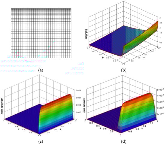
Grid NumberBCD on Uniform GridsBCD on Nonuniform Grids
ErrorRateCPUErrorRateCPU
ε = 0.1
1632.30 × 10−6 377.021.20 × 10−6 368.76
2431.71 × 10−76.41945.708.65 × 10−86.48935.80
3232.56 × 10−86.601979.741.27 × 10−86.671938.75
4035.84 × 10−96.623294.522.88 × 10−96.653267.10
6432.46 × 10−106.7311,497.211.21 × 10−106.7411,607.82
ε = 0.05
1633.57 × 10−4 370.281.71 × 10−5 349.66
2433.46 × 10−65.751434.505.28 × 10−78.58892.31
3236.01 × 10−66.081881.507.73 × 10−86.681948.70
4031.48 × 10−66.283121.331.69 × 10−86.813184.98
6437.04 × 10−86.4811,867.196.97 × 10−106.7812,392.76
ε = 0.01
1632.59 × 10−11.37449.881.56 × 10−47.59534.23
2439.99 × 10−22.351085.342.99 × 10−54.071041.01
3233.99 × 10−22.702191.687.08 × 10−64.462360.45
4031.71 × 10−23.803647.552.08 × 10−65.493771.67
6432.00 × 10−34.3221,577.831.39 × 10−75.7622,842.95
Table 7. Comparison of the maximum absolute error and convergence rate between the BCD scheme and the HOC scheme [34] on nonuniform grids for Problem 3.
Grid NumberHOC [34] on Nonuniform GridsBCD on Nonuniform Grids
ErrorRateErrorRate
ε = 0.1
1633.13 × 10−5 1.30 × 10⁻⁵
3231.97 × 10−63.991.25 × 10−76.70
6431.23 × 10−74.001.12 × 10−96.80
ε = 0.05
1632.28 × 10−4 4.38 × 10⁻⁵
3231.40 × 10−54.039.09 × 10−75.59
6438.68 × 10−74.011.82 × 10−85.64
ε = 0.01
1635.54 × 10−3 3.63 × 10⁻³
3233.37 × 10−44.048.68 × 10−55.39
6432.11 × 10−54.001.52 × 10−65.84
Table 8. Comparison of the maximum absolute error and convergence rate between the BCD scheme and the HOC scheme [34] on uniform grids for Problem 3.
Grid NumberHOC [34] on Uniform GridsBCD on Uniform Grids
ErrorRateErrorRate
ε = 0.1
1636.17 × 10−4 5.09 × 10⁻⁴
3233.91 × 10−53.988.01 × 10−65.99
6432.46 × 10−63.998.96 × 10−86.48
ε = 0.05
1639.90 × 10−3 1.74 × 10⁻²
3236.48 × 10−43.935.10 × 10−45.09
6434.10 × 10−53.988.01 × 10−45.99
Table 9. Comparison of the maximum absolute error and convergence rate on uniform grids and nonuniform grids for Problem 3.
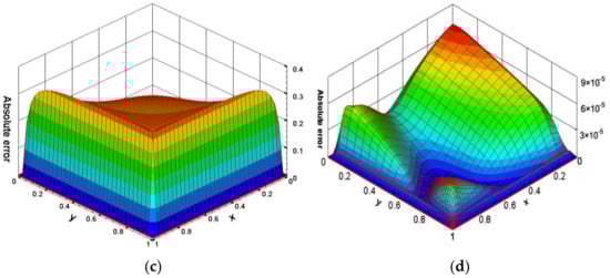
Grid NumberBCD on Uniform GridsBCD on Nonuniform Grids
ErrorRateErrorRate
ε = 0.1
1635.09 × 10−4 1.30 × 10⁻⁵
2434.66 × 10−55.898.58 × 10−76.70
3238.01 × 10−66.121.25 × 10−76.69
4031.92 × 10−66.402.74 × 10−86.80
6438.96 × 10−86.521.12 × 10−96.80
ε = 0.05
1631.74 × 10−2 4.38 × 10⁻⁵
2432.35 × 10−34.945.84 × 10−64.97
3235.10 × 10−45.309.09 × 10−76.47
4031.39 × 10−45.821.77 × 10−77.33
6438.01 × 10−66.071.82 × 10−84.84
ε = 0.01
1638.97 × 10−1 3.63 × 10⁻³
2436.60 × 10−10.764.45 × 10−45.18
3233.79 × 10−11.938.68 × 10−55.68
4033.80 × 10−10.012.52 × 10−55.54
6434.49 × 10−24.541.52 × 10−65.97
Disclaimer/Publisher’s Note: The statements, opinions and data contained in all publications are solely those of the individual author(s) and contributor(s) and not of MDPI and/or the editor(s). MDPI and/or the editor(s) disclaim responsibility for any injury to people or property resulting from any ideas, methods, instructions or products referred to in the content.

