Developments of Efficient Trigonometric Quantile Regression Models for Bounded Response Data

Abstract

The choice of an appropriate regression model for econometric modeling minimizes information loss and also leads to sound inferences. In this study, we develop four quantile regression models based on trigonometric extensions of the unit generalized half-normal distributions for the modeling of a bounded response variable defined on the unit interval. The desirable shapes of these distributions, such as left-skewed, right-skewed, reversed-J, approximately symmetric, and bathtub shapes, make them competitive models for bounded responses with such traits. The maximum likelihood method is used to estimate the parameters of the regression models, and Monte Carlo simulation results confirm the efficiency of the method. We demonstrate the utility of our models by investigating the relationship between OECD countries’ educational attainment levels, labor market insecurity, and homicide rates. The diagnostics reveal that all our models provide a good fit to the data because the residuals are well behaved. A comparative analysis of the trigonometric quantile regression models with the unit generalized half-normal quantile regression model shows that the trigonometric models are the best. However, the sine unit generalized half-normal (SUGHN) quantile regression model is the best overall. It is observed that labor market insecurity and the homicide rate have significant negative effects on the educational attainment values of the OECD countries.

1. Introduction

Regression analyses are very instrumental in the econometric modeling of the relationship between a response variable and a set of covariates or exogenous variables. The regression models adopted for such analysis can either be parametric or non-parametric in nature. However, when we are certain about the distribution of the response variable, the parametric regression model is preferred over the non-parametric model. Due to this, the development of parametric regression models using (statistical or probability) distributions is on the rise.

Due to their applicability in the fields of psychology, environment, epidemiology, finance, education, and economics, among others, numerous regression models for examining relationships between an endogenous variable defined on the unit interval and exogenous variables have been developed more recently. Basically, they aim to model the conditional mean of the response variable. Among them, the beta regression model developed in [1] is the most utilized because of the easy interpretation of the estimated coefficients. Despite the flexibility of the beta regression model, the literature has been flooded with other regression models using distributions defined on the unit interval. They include the Vasicek regression model [2], log-weighted exponential regression model [3], log-Bilal regression model [4], unit improved second-degree Lindley regression model [5], and the unit Lindley regression model [6], among others.

When the bounded response variable is non-symmetric or contaminated with outliers, the appropriateness of the regression model based on the conditional mean becomes questionable. This is because the mean is not a robust measure of central tendency due to its susceptibility to outliers. Thus, quantile regression models have been proposed as alternatives; thanks to their robustness, they are suitable when the response variable is skewed or contaminated by outliers. In light of this, many quantile regression models for modeling the conditional quantile of the response variable defined on the unit interval have been developed using bounded distributions. Examples include the Vasicek quantile regression model [2], unit generalized half-normal (UGHN) quantile regression model [7], unit exponentiated Fréchet quantile regression model [8], unit gamma/Gompertz quantile regression model [9], generalized Topp-Leone median regression model [10], unit log-log quantile regression model [11], and the new unit Burr XII quantile regression model [12].

Although several bounded quantile regression models exist in the literature, none can be said to handle all the complex characteristics of data generated on a daily basis. As a result, the ongoing creation of new models facilitates data analysis with little information loss. In this study, we propose four new quantile regression models for the modeling of a bounded response variable using trigonometric classes of distributions and the UGHN distribution. The choice of trigonometric classes for modifying the UGHN distribution before developing the quantile regression model comes from the fact that they are parsimonious, simple to handle, and provide excellent parametric fit (see [13,14]). On the other hand, the UGHN distribution has proved itself as a flexible and adaptive distribution that can serve to construct efficient fit and regression models (see [7,15]). The motivations behind combining the functionalities of trigonometric classes with the UGHN distribution are thus to provide parsimonious quantile regression models capable of modeling a bounded response variable that exhibits left-skewed, right-skewed, approximately symmetric, reversed-J, J, and bathtub probability density shapes, and also to offer a heavy-tailed quantile regression model for modeling a bounded response.

The article is structured into eight sections. Section 2 describes the preliminary knowledge. The trigonometric forms of the UGHN distribution are indicated in Section 3. Section 4 develops the quantile densities of the trigonometric forms of the UGHN distribution. Section 5 presents the proposed quantile regression models, parameter estimation method and residual analysis. Section 6 is devoted to the Monte Carlo simulations. An empirical illustration of the developed models is given in Section 7. The conclusion is finally presented in Section 8.

2. Preliminary Knowledge

2.1. Trigonometric Classes of Distributions

Trigonometric classes of distributions have been useful in recent times for modifying existing classical distributions. In a Ph.D. thesis in 2015, Souza [14] derived some simple and novel trigonometric classes for changing the functional structure of standard distributions, which were later refined in [16,17,18,19]. These include the sin-G, cos-G, tan-G, and sec-G classes. For the purposes of this study, a mathematical presentation of these classes is now presented. Let $G(y;\eta )$ and $\mathrm{g}(y;\eta )$ denote the cumulative distribution function (CDF) and probability density function (PDF) of a continuous distribution, respectively, and $\eta$ denotes a vector of parameters. According to [16], the CDF and PDF of the sin-G class are, respectively, given by

$$\begin{array}{c}\hfill F(y;\eta )=sin\left[\frac{\pi }{2}G(y;\eta )\right],y\in \mathbb{R}\end{array}$$

(1)

and

$$\begin{array}{c}\hfill f(y;\eta )=\frac{\pi }{2}\mathrm{g}(y;\eta )cos\left[\frac{\pi }{2}G(y;\eta )\right].\end{array}$$

(2)

According to [17], the CDF and PDF of the cos-G class are, respectively, defined as

$$\begin{array}{c}\hfill F(y;\eta )=1-cos\left[\frac{\pi }{2}G(y;\eta )\right],y\in \mathbb{R}\end{array}$$

(3)

and

$$\begin{array}{c}\hfill f(y;\eta )=\frac{\pi }{2}\mathrm{g}(y;\eta )sin\left[\frac{\pi }{2}G(y;\eta )\right].\end{array}$$

(4)

With reference to [18] (or [20]), the CDF and PDF of the tan-G class are, respectively, given by

$$\begin{array}{c}\hfill F(y;\eta )=tan\left[\frac{\pi }{4}G(y;\eta )\right],y\in \mathbb{R}\end{array}$$

(5)

and

$$\begin{array}{c}\hfill f(y;\eta )=\frac{\pi }{4}\mathrm{g}(y;\eta ){sec}^2\left[\frac{\pi }{4}G(y;\eta )\right].\end{array}$$

(6)

Finally, Souza et al. [19] defined the CDF and PDF of the sec-G class as, respectively,

$$\begin{array}{c}\hfill F(y;\eta )=sec\left[\frac{\pi }{3}G(y;\eta )\right]-1,y\in \mathbb{R}\end{array}$$

(7)

and

$$\begin{array}{c}\hfill f(y;\eta )=\frac{\pi }{3}\mathrm{g}(y;\eta )sec\left[\frac{\pi }{3}G(y;\eta )\right]tan\left[\frac{\pi }{3}G(y;\eta )\right].\end{array}$$

(8)

The merits of these trigonometric classes are that there is no addition of parameters to the baseline distribution; the trigonometric function confers an original oscillating feature to the probability functions, mainly the PDF and hazard rate function; these functions are quite simple from a mathematical viewpoint; and it projects a different modeling target than the baseline distribution. To illustrate this last point, the sin-G class and its baseline distribution have the following comprehensive first-order stochastic ordering: $F(y,\eta )\ge G(y,\eta )$ for any $y\in \mathbb{R}$. Further developments on trigonometric classes can be found in the survey of [21]. Some specific lifetime distributions based on these classes have been the subject of full publications. See, for example, the sin-exponential distribution in [22], sin-Weibull, cos-Weibull, and tan-Weibull distributions in [13], sin-Fréchet distribution in [23], sin-inverse Rayleigh distribution in [24], and the sin-Nadarajah-Haghighi distribution in [25]. To the best of our knowledge, in the context of these trigonometric classes, the consideration of bounded baseline distributions and the construction of efficient quantile regression models based on them have been unexplored.

2.2. UGHN Distribution

The mathematical foundations of the UGHN distribution, which were sketched in the introduction, are presented in this section. To begin, the UGHN distribution is a unit distribution created in [15]. In the functional aspect, it depends on two parameters, $\gamma >0$ and $\beta >0$, and corresponds to the distribution of $Y=e^{-X}$, where X denotes a random variable following the classical generalized half-normal distribution with parameters $\gamma$ and $\beta$ (introduced in [26]). The CDF and PDF of Y are, respectively, given by

$$\begin{array}{c}\hfill G(y;\gamma ,\beta )=2\Phi \left(-{\left(-\frac{log\left(y\right)}{\gamma }\right)}^{\beta }\right),0<y<1\end{array}$$

(9)

and

$$\begin{array}{c}\hfill \mathrm{g}(y;\gamma ,\beta )=\sqrt{\frac{2}{\pi }}\frac{\beta }{y(-log(y\left)\right)}{\left(-\frac{log\left(y\right)}{\gamma }\right)}^{\beta }exp\left[-\frac{1}{2}{\left(-\frac{log\left(y\right)}{\gamma }\right)}^{2\beta }\right],\end{array}$$

(10)

where $\Phi (·)$ is the CDF of the standard normal distribution. The UGHN distribution is a flexible distribution with a thicker left tail than the Weibull, gamma, and lognormal distributions. In addition, it can exhibit both left and right-skewness for given parameter values. The UGHN distribution’s desirable properties have made it a viable candidate for modeling lifetime data (see [15]). It is also desirable in the applied context of quantile regression modeling (see [7]).

3. Trigonometric UGHN Distributions

In this section, based on the material presented in the above sections, we propose four trigonometric distributions. These are the sin-UGHN (SUGHN), cos-UGHN (CUGHN), tan-UGHN (TUGHN), and sec-UGHN (SCUGHN) distributions.

3.1. SUGHN Distribution

Combining Equations (1), (2), (9), and (10), the CDF and PDF of the SUGHN distribution are, respectively, given by

$$\begin{array}{c}\hfill F(y;\gamma ,\beta )=sin\left[\pi \Phi \left(-{\left(-\frac{log\left(y\right)}{\gamma }\right)}^{\beta }\right)\right],0<y<1\end{array}$$

(11)

and

$$\begin{array}{cc}\hfill f(y;\gamma ,\beta )& =\sqrt{\frac{\pi }{2}}\frac{\beta }{y(-log(y\left)\right)}{\left(-\frac{log\left(y\right)}{\gamma }\right)}^{\beta }exp\left[-\frac{1}{2}{\left(-\frac{log\left(y\right)}{\gamma }\right)}^{2\beta }\right]\times \hfill \\ \hfill & cos\left[\pi \Phi \left(-{\left(-\frac{log\left(y\right)}{\gamma }\right)}^{\beta }\right)\right].\hfill \end{array}$$

(12)

The PDF plots of the SUGHN distribution for some selected values of the parameters are shown in Figure 1. These plots display left-skewed, right-skewed, approximately symmetric, reversed-J, and bathtub shapes. This makes the SUGHN distribution suitable for modeling data with these traits.

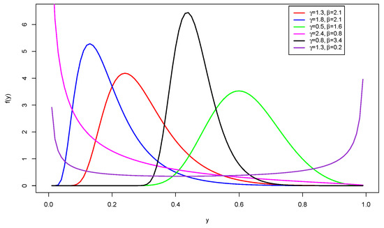
Figure 1. PDF plots of the SUGHN distribution.

The quantile function (QF) (or the inverse CDF) is very useful when generating random observations from the distribution and also for computing measures of shape and dispersion. The QF of the SUGHN distribution is

$$\begin{array}{c}\hfill Q(p;\gamma ,\beta )=exp\left[-\gamma {\left(-{\Phi }^{-1}\left(\frac{arcsin\left(p\right)}{\pi }\right)\right)}^{1/\beta }\right],0<p<1.\end{array}$$

(13)

3.2. CUGHN Distribution

The CDF and PDF of the CUGHN distribution are obtained by combining Equations (3), (4), (9), and (10). Thus, the CDF is given by

$$\begin{array}{c}\hfill F(y;\gamma ,\beta )=1-cos\left[\pi \Phi \left(-{\left(-\frac{log\left(y\right)}{\gamma }\right)}^{\beta }\right)\right],0<y<1.\end{array}$$

(14)

The corresponding PDF is given by

$$\begin{array}{cc}\hfill f(y;\gamma ,\beta )& =\sqrt{\frac{\pi }{2}}\frac{\beta }{y(-log(y\left)\right)}{\left(-\frac{log\left(y\right)}{\gamma }\right)}^{\beta }exp\left[-\frac{1}{2}{\left(-\frac{log\left(y\right)}{\gamma }\right)}^{2\beta }\right]\times \hfill \\ \hfill & sin\left[\pi \Phi \left(-{\left(-\frac{log\left(y\right)}{\gamma }\right)}^{\beta }\right)\right].\hfill \end{array}$$

(15)

The PDF plots of the CUGHN distribution displayed in Figure 2 exhibit left-skewed, right-skewed, reversed-J, and bathtub shapes. However, they do not display the approximately symmetric shape shown by the SUGHN distribution. Hence, this distribution is capable of modeling data with such characteristics.

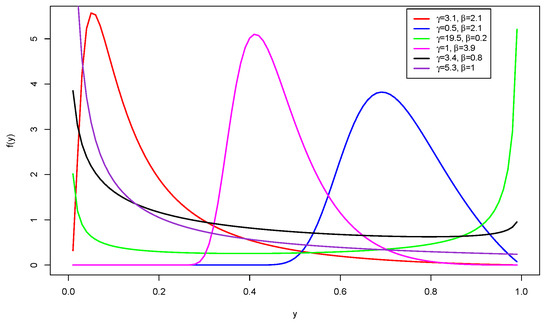
Figure 2. PDF plots of the CUGHN distribution.

The corresponding QF is

$$\begin{array}{c}\hfill Q(p;\gamma ,\beta )=exp\left[-\gamma {\left(-{\Phi }^{-1}\left(\frac{arccos(1-p)}{\pi }\right)\right)}^{1/\beta }\right],0<p<1.\end{array}$$

(16)

3.3. TUGHN Distribution

The TUGHN distribution is developed using Equations (5), (6), (9), and (10). Hence, the corresponding CDF and PDF are, respectively, given by

$$\begin{array}{c}\hfill F(y;\gamma ,\beta )=tan\left[\frac{\pi }{2}\Phi \left(-{\left(-\frac{log\left(y\right)}{\gamma }\right)}^{\beta }\right)\right],0<y<1\end{array}$$

(17)

and

$$\begin{array}{cc}\hfill f(y;\gamma ,\beta )& =\sqrt{\frac{\pi }{8}}\frac{\beta }{y(-log(y\left)\right)}{\left(-\frac{log\left(y\right)}{\gamma }\right)}^{\beta }exp\left[-\frac{1}{2}{\left(-\frac{log\left(y\right)}{\gamma }\right)}^{2\beta }\right]\times \hfill \\ \hfill & {sec}^2\left[\frac{\pi }{2}\Phi \left(-{\left(-\frac{log\left(y\right)}{\gamma }\right)}^{\beta }\right)\right],\hfill \end{array}$$

(18)

respectively. The PDF plots of the TUGHN distribution in Figure 3 show left-skewed, right-skewed, reversed-J, J, and bathtub shapes. Although the TUGHN distribution does not show the approximate symmetric shape displayed by the SUGHN, it has an increasing or J shape that is not exhibited by the SUGHN and CUGHN distributions. Hence, the TUGHN distribution is a candidate for modeling bounded data with such characteristics.

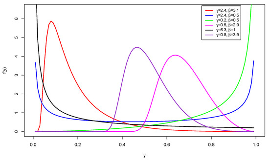
Figure 3. PDF plots of the TUGHN distribution.

The corresponding QF is

$$\begin{array}{c}\hfill Q(p;\gamma ,\beta )=exp\left[-\gamma {\left(-{\Phi }^{-1}\left(\frac{2arctan\left(p\right)}{\pi }\right)\right)}^{1/\beta }\right],0<p<1.\end{array}$$

(19)

3.4. SCUGHN Distribution

The CDF and PDF of the SCUGHN distribution are developed by substituting Equation (9) into (7) and, Equations (10) and (9) into (8). Therefore, the corresponding CDF is given by

$$\begin{array}{c}\hfill F(y;\gamma ,\beta )=sec\left[\frac{2\pi }{3}\Phi \left(-{\left(-\frac{log\left(y\right)}{\gamma }\right)}^{\beta }\right)\right]-1,0<y<1.\end{array}$$

(20)

The associated PDF is

$$\begin{array}{cc}\hfill f(y;\gamma ,\beta )=& \sqrt{\frac{2\pi }{9}}\frac{\beta }{y(-log(y\left)\right)}{\left(-\frac{log\left(y\right)}{\gamma }\right)}^{\beta }exp\left[-\frac{1}{2}{\left(-\frac{log\left(y\right)}{\gamma }\right)}^{2\beta }\right]\times \hfill \\ & sec\left[\frac{2\pi }{3}\Phi \left(-{\left(-\frac{log\left(y\right)}{\gamma }\right)}^{\beta }\right)\right]tan\left[\frac{2\pi }{3}\Phi \left(-{\left(-\frac{log\left(y\right)}{\gamma }\right)}^{\beta }\right)\right].\hfill \end{array}$$

(21)

Figure 4 shows that the SCUGHN distribution can exhibit left-skewed, right-skewed, reversed-J, and bathtub shapes for some given parameter values. The SCUGHN distribution shows similar shapes to the CUGHN distribution.

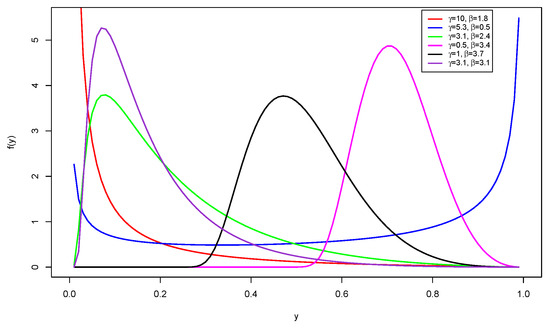
Figure 4. PDF plots of the SCUGHN distribution.

The corresponding QF is

$$\begin{array}{c}\hfill Q(p;\gamma ,\beta )=exp\left[-\gamma {\left(-{\Phi }^{-1}\left(\frac{3arcsec(p+1)}{2\pi }\right)\right)}^{1/\beta }\right],0<p<1.\end{array}$$

(22)

4. Quantile PDFs of the Trigonometric Forms of the UGHN Distribution

In order to develop the quantile regression models for the SUGHN, CUGHN, TUGHN, and SCUGHN distributions, it is essential to parametrize their PDF in terms of the $100pth$ quantile, $\mu =Q(p;\gamma ,\beta )$. To do this, we make $\gamma$ the subject in the QFs of the SUGHN, CUGHN, TUGHN, and SCUGHN distributions and substitute them in their corresponding PDFs. To get the quantile PDF of the SUGHN distribution, we substitute $\gamma =-log\left(\mu \right){(-{\Phi }^{-1}(arcsin\left(p\right)/\pi ))}^{-1/\beta }$ into Equation (12). The quantile PDF is calculated as follows:

$$\begin{array}{cc}\hfill f(y;\mu ,p,\beta )=& \sqrt{\frac{\pi }{2}}\frac{\beta {\Phi }^{-1}(arcsin\left(p\right)/\pi )}{ylog\left(y\right)}{\left(\frac{log\left(y\right)}{log\left(\mu \right)}\right)}^{\beta }\times \hfill \\ & exp\left[-\frac{1}{2}{\left[{\Phi }^{-1}\left(\frac{arcsin\left(p\right)}{\pi }\right)\right]}^2{\left(\frac{log\left(y\right)}{log\left(\mu \right)}\right)}^{2\beta }\right]\times \hfill \\ & cos\left[\pi \Phi \left({\Phi }^{-1}\left(\frac{arcsin\left(p\right)}{\pi }\right){\left(\frac{log\left(y\right)}{log\left(\mu \right)}\right)}^{\beta }\right)\right],0<y<1,\hfill \end{array}$$

(23)

where $\beta >0$ is the shape parameter, $\mu$ is the quantile parameter, and p satisfies $0<p<1$.

Similarly, the quantile PDF of the CUGHN distribution is obtained by substituting $\gamma =-log\left(\mu \right){(-{\Phi }^{-1}(arccos\left(p\right)/\pi ))}^{-1/\beta }$ into Equation (15). It is thus given by

$$\begin{array}{cc}\hfill f(y;\mu ,p,\beta )=& \sqrt{\frac{\pi }{2}}\frac{\beta {\Phi }^{-1}(arccos(1-p)/\pi )}{ylog\left(y\right)}{\left(\frac{log\left(y\right)}{log\left(\mu \right)}\right)}^{\beta }\times \hfill \\ & exp\left[-\frac{1}{2}{\left[{\Phi }^{-1}\left(\frac{arccos(1-p)}{\pi }\right)\right]}^2{\left(\frac{log\left(y\right)}{log\left(\mu \right)}\right)}^{2\beta }\right]\times \hfill \\ & sin\left[\pi \Phi \left({\Phi }^{-1}\left(\frac{arccos(1-p)}{\pi }\right){\left(\frac{log\left(y\right)}{log\left(\mu \right)}\right)}^{\beta }\right)\right],0<y<1.\hfill \end{array}$$

(24)

To obtain the quantile PDF of the TUGHN distribution, we substitute

$\gamma =-log\left(\mu \right){(-{\Phi }^{-1}(2arctan\left(p\right)/\pi ))}^{-1/\beta }$ into Equation (18). This PDF is thus given by

$$\begin{array}{cc}\hfill f(y;\mu ,p,\beta )=& \sqrt{\frac{\pi }{8}}\frac{\beta {\Phi }^{-1}(2arctan\left(p\right)/\pi )}{ylog\left(y\right)}{\left(\frac{log\left(y\right)}{log\left(\mu \right)}\right)}^{\beta }\times \hfill \\ & exp\left[-\frac{1}{2}{\left[{\Phi }^{-1}\left(\frac{2arctan\left(p\right)}{\pi }\right)\right]}^2{\left(\frac{log\left(y\right)}{log\left(\mu \right)}\right)}^{2\beta }\right]\times \hfill \\ & {sec}^2\left[\frac{\pi }{2}\Phi \left({\Phi }^{-1}\left(\frac{2arctan\left(p\right)}{\pi }\right){\left(\frac{log\left(y\right)}{log\left(\mu \right)}\right)}^{\beta }\right)\right],0<y<1.\hfill \end{array}$$

(25)

Substituting $\gamma =-log\left(\mu \right){(-{\Phi }^{-1}(3arcsec(p+1)/2\pi ))}^{-1/\beta }$ into Equation (21) yields the quantile PDF of the SCUGHN distribution, which is given by

$$\begin{array}{cc}\hfill f(y;\mu ,p,\beta )=& \sqrt{\frac{2\pi }{9}}\frac{\beta {\Phi }^{-1}(3arcsec(p+1)/2\pi )}{ylog\left(y\right)}{\left(\frac{log\left(y\right)}{log\left(\mu \right)}\right)}^{\beta }\times \hfill \\ & exp\left[-\frac{1}{2}{\left[{\Phi }^{-1}\left(\frac{3arcsec(p+1)}{2\pi }\right)\right]}^2{\left(\frac{log\left(y\right)}{log\left(\mu \right)}\right)}^{2\beta }\right]\times \hfill \\ & sec\left[\frac{2\pi }{3}\Phi \left({\Phi }^{-1}\left(\frac{3arcsec(p+1)}{2\pi }\right){\left(\frac{log\left(y\right)}{log\left(\mu \right)}\right)}^{\beta }\right)\right]\times \hfill \\ & tan\left[\frac{2\pi }{3}\Phi \left({\Phi }^{-1}\left(\frac{3arcsec(p+1)}{2\pi }\right){\left(\frac{log\left(y\right)}{log\left(\mu \right)}\right)}^{\beta }\right)\right],0<y<1.\hfill \end{array}$$

(26)

The quantile PDFs given in Equations (23)–(26) form the basis of our quantile regression models. Indeed, the SUGHN quantile regression model is obtained using Equation (23), the CUGHN quantile regression model is obtained using Equation (24), the TUGHN quantile regression model is obtained using Equation (25), and the SCUGHN quantile regression model is obtained using Equation (26).

5. Quantile Regression Model, Estimation and Residual Analysis

5.1. Quantile Regression Model

This section presents the quantile regression model for the proposed trigonometric distributions. Consider n independent realizations of a random variable Y that follows the SUGHN, CUGHN, TUGHN, or SCUGHN distributions (depending on the context), denoted by $y_1,y_2,\dots ,y_n$. The quantile regression models are developed using the logit link function. Thus, for any $i=1,2,\dots ,n$, we set

$$\begin{array}{c}\hfill {\mu }_i={\mathrm{h}}^{-1}\left({\mathit{x}}_i^{\mathrm{T}}\rho \right),\end{array}$$

(27)

where $\mathrm{h}(·)$ is the logit link function used to link the conditional quantile of the dependent variable to the independent variables, $\rho ={({\rho }_0,{\rho }_1,\dots ,{\rho }_p)}^{\mathrm{T}}$ is the vector of unknown parameters, and ${\mathit{x}}_i^{\mathrm{T}}=(1,x_{i1},x_{i2},\dots ,x_{ip})$ are the known i-th vector of independent variables. Although several link functions exist, we adopt the logit link function because of its simplicity when interpreting the coefficients of the independent variables. As a result, the model can be written as

$$\begin{array}{c}\hfill \mathrm{logit}\left({\mu }_i\right)=log\left(\frac{{\mu }_i}{1-{\mu }_i}\right)={\rho }_0+{\rho }_1{x}_{i1}+{\rho }_2{x}_{i2}+\dots +{\rho }_p{x}_{ip}.\end{array}$$

(28)

It is important to note that, for $j=1,2,\dots ,p$, when $x_{ij}$ is continuous, a unit increase causes $100\%\times (e^{{\rho }_j}-1)$ change in the conditional quantile of the dependent variable, while the other independent variables remain constant. When $x_{ij}$ is a categorical variable, a unit increase results in a $100\%\times e^{{\rho }_j}$ change in the conditional quantile of the dependent variable from $x_{ij}=1$ to $x_{ij}=0$, while the other independent variables remain constant. Setting $p=0.5$ yields the median regression. See [2,7,8,9] and [11] for more information on the formulation of quantile regression models with bounded distributions.

5.2. Parameter Estimation

This section describes the parameter estimation method and inference conducted using the classical maximum likelihood estimation approach. Consider n independent realizations of a random variable Y that follows the SUGHN, CUGHN, TUGHN, or SCUGHN distributions (depending on the context), denoted by $y_1,y_2,\dots ,y_n$ and the vector of the involved parameters, denoted by $\phi ={(\mu ,p,\beta )}^{\mathrm{T}}$. Then, the log-likelihood function is given by

$$\begin{array}{c}\hfill \ell \left(\phi \right|y)=\sum _{i=1}^{n}logf(y_i;{\mu }_i,p,\beta ),\end{array}$$

(29)

where $f(·)$ is the corresponding quantile PDF and $y=(y_1,y_2,\dots ,y_n)$. The maximum likelihood estimates are obtained by maximizing the function

$$\begin{array}{c}\hfill \widehat{\phi }=\arg \left[\underset{\phi \in \Omega }{sup}\ell \left(\phi \right|y)\right],\end{array}$$

(30)

where $\Omega$ is the parameter space of $\phi$. For the models in Equations (23)–(26), it is not possible to obtain closed form solutions for the maximum likelihood estimates of parameters. Thus, numerical solutions are employed using the BFGS algorithm in the R software [27]. The standard errors of the estimates of the parameters are determined using the large sample property of the maximum likelihood method (see [28]). The observed Fisher information matrix used to estimate standard errors for the parameters is given by

$$\begin{array}{c}\hfill \mathrm{I}\left(\widehat{\phi }\right)=-{\left.\frac{\partial \ell \left(\phi \right|y)}{\partial {\phi }^{\mathrm{T}}\partial {\phi }^{\mathrm{T}}}\right|}_{\phi =\widehat{\phi }}.\end{array}$$

5.3. Residual Analysis

To examine the adequacy of a fitted quantile regression model, it is important to investigate the behavior of its residuals. In this study, we adopt the randomized quantile residuals developed in [29]. They are defined as

$$\begin{array}{c}\hfill r_i={\Phi }^{-1}\left[F(y_i;\widehat{\phi })\right],i=1,2,\dots ,n,\end{array}$$

where $F(·)$ is the corresponding estimated quantile CDF and ${\Phi }^{-1}(·)$ is the quantile of the standard normal distribution. If the model fits the data well, then it is expected that the randomized quantile residuals will follow the standard normal distribution.

6. Monte Carlo Simulations

In this section, Monte Carlo simulation experiments are performed to investigate the properties of the maximum likelihood estimates. We take $p=2$ and the experiments are repeated $N=5000$ times using sample sizes of $n=25,50,100,150$, and 200. The following two parameter combinations are used in the experiment: $({\rho }_0,{\rho }_1,{\rho }_2,\beta )=(0.2,0.1,0.8,0.3)$ and $({\rho }_0,{\rho }_1,{\rho }_2,\beta )=(0.1,0.7,0.4,0.5)$. For each parameter combination, the following regression structure is employed during the simulation:

$$\begin{array}{c}\hfill log\left(\frac{{\mu }_i}{1-{\mu }_i}\right)={\rho }_0+{\rho }_1{x}_{i1}+{\rho }_2{x}_{i2},\end{array}$$

where $x_{i1}$ is a realization from a standard uniform distribution and $x_{i2}$ is a realization from a four-degree-of-freedom student distribution. The independent variables remain fixed throughout the simulations. The observations for the response variable for a given quantile regression model are obtained using its corresponding distribution. Hence, for the various quantile regression models proposed, the response variable observations are generated using the following:

• For the SUGHN distribution, for any $i=1,2,\dots ,n$, we consider

  $$\begin{array}{c}\hfill y_i=exp\left[-{\gamma }_i{\left(-{\Phi }^{-1}\left(\frac{arcsin\left(u_i\right)}{\pi }\right)\right)}^{1/\beta }\right],\end{array}$$

  where ${\gamma }_i=-log\left({\mu }_i\right){(-{\Phi }^{-1}(arcsin\left(p\right)/\pi ))}^{-1/\beta }$ and $u_i$ is an observation from the standard uniform distribution.
• For the CUGHN distribution, we consider

  $$\begin{array}{c}\hfill y_i=exp\left[-{\gamma }_i{\left(-{\Phi }^{-1}\left(\frac{arccos(1-u_i)}{\pi }\right)\right)}^{1/\beta }\right],\end{array}$$

  where ${\gamma }_i=-log\left({\mu }_i\right){(-{\Phi }^{-1}(arccos\left(p\right)/\pi ))}^{-1/\beta }$.
• For the TUGHN distribution, we consider

  $$\begin{array}{c}\hfill y_i=exp\left[-{\gamma }_i{\left(-{\Phi }^{-1}\left(\frac{2arctan\left(u_i\right)}{\pi }\right)\right)}^{1/\beta }\right],\end{array}$$

  where ${\gamma }_i=-log\left({\mu }_i\right){(-{\Phi }^{-1}(2arctan\left(p\right)/\pi ))}^{-1/\beta }$.
• For the SCUGHN distribution, we consider

  $$\begin{array}{c}\hfill y_i=exp\left[-{\gamma }_i{\left(-{\Phi }^{-1}\left(\frac{3arcsec(u_i+1)}{2\pi }\right)\right)}^{1/\beta }\right],\end{array}$$

  where ${\gamma }_i=-log\left({\mu }_i\right){(-{\Phi }^{-1}(3arcsec(p+1)/2\pi ))}^{-1/\beta }$.

The simulation is carried out using the median regression by setting $p=0.5$. The performance of the estimates is examined using the absolute bias (AB) and root mean square error (RMSE), which are, respectively, given by

$$\begin{array}{c}\hfill \mathrm{AB}=\frac{1}{N}\sum _{i=1}^N|{\widehat{\phi }}_i-\phi |\end{array}$$

and

$$\begin{array}{c}\hfill \mathrm{RMSE}=\sqrt{\frac{1}{N}\sum _{i=1}^N{({\widehat{\phi }}_i-\phi )}^2},\end{array}$$

where $\phi ={\rho }_0,{\rho }_1,{\rho }_2$ or $\beta$. We also compute the average estimates (AEs) of the parameters. According to Table 1 and Table 2, the AEs approach the true parameter values as the sample size increases. The ABs and RMSEs decrease as the sample size increases. The results from our Monte Carlo simulation agree with the large sample property of the maximum likelihood method. Thus, the estimates of the parameters are consistent.

Table 1. Simulations results for $({\rho }_0,{\rho }_1,{\rho }_2,\beta )=(0.2,0.1,0.8,0.3)$.

Parameter	n	SUGHN			CUGHN			TUGHN			SCUGHN
		AE	AB	RMSE	AE	AB	RMSE	AE	AB	RMSE	AE	AB	RMSE
${\rho }_0$	25	0.2199	0.2611	0.3371	0.3131	0.3391	0.4645	0.3413	0.3645	0.5001	0.3646	0.3725	0.5218
	50	0.1989	0.2272	0.2814	0.2482	0.2758	0.3674	0.2708	0.2933	0.3970	0.2907	0.2874	0.4122
	100	0.1813	0.1928	0.2306	0.1938	0.2265	0.2812	0.2061	0.2349	0.3012	0.2186	0.2093	0.2938
	150	0.1771	0.1734	0.2034	0.1844	0.2093	0.2559	0.1943	0.2188	0.2752	0.2080	0.1795	0.2630
	200	0.1692	0.1578	0.1827	0.1834	0.1930	0.2310	0.1908	0.1978	0.2446	0.2006	0.1501	0.2209
${\rho }_1$	25	0.3508	0.3667	0.5715	0.3840	0.4076	0.6396	0.4060	0.4269	0.6664	0.4106	0.4256	0.6736
	50	0.2804	0.2949	0.4585	0.3486	0.3661	0.5738	0.3656	0.3837	0.6017	0.3580	0.3645	0.5953
	100	0.2476	0.2531	0.3785	0.2495	0.2705	0.4263	0.2606	0.2798	0.4505	0.2471	0.2483	0.4411
	150	0.2033	0.2109	0.3118	0.2584	0.2647	0.3990	0.2700	0.2774	0.4254	0.2434	0.2279	0.4028
	200	0.2059	0.2043	0.2857	0.2345	0.2352	0.3498	0.2448	0.2433	0.3737	0.2203	0.1909	0.3470
${\rho }_2$	25	0.8129	0.3233	0.3976	0.7769	0.4018	0.4743	0.7753	0.4297	0.4997	0.7407	0.4393	0.5159
	50	0.8129	0.2259	0.2860	0.8055	0.3024	0.3780	0.8027	0.3289	0.4062	0.7692	0.3292	0.4198
	100	0.8002	0.1564	0.1994	0.8148	0.2081	0.2654	0.8109	0.2234	0.2893	0.7841	0.2120	0.2959
	150	0.8069	0.1234	0.1572	0.8096	0.1679	0.2141	0.8083	0.1811	0.2325	0.7784	0.1603	0.2305
	200	0.8027	0.1093	0.1388	0.8085	0.1417	0.1830	0.8040	0.1499	0.1976	0.7808	0.1263	0.1930
$\beta$	25	0.3193	0.0398	0.0539	0.3139	0.0376	0.0491	0.3132	0.0351	0.0460	0.3158	0.0340	0.0461
	50	0.3100	0.0271	0.0346	0.3057	0.0257	0.0328	0.3052	0.0240	0.0307	0.3075	0.0218	0.0297
	100	0.3041	0.0184	0.0232	0.3027	0.0177	0.0229	0.3025	0.0163	0.0213	0.3043	0.0137	0.0197
	150	0.3031	0.0147	0.0186	0.3030	0.0147	0.0188	0.3027	0.0135	0.0174	0.3041	0.0105	0.0155
	200	0.3021	0.0128	0.0162	0.3006	0.0119	0.0153	0.3005	0.0109	0.0142	0.3017	0.0080	0.0121

Table 2. Simulations results for $({\rho }_0,{\rho }_1,{\rho }_2,\beta )=(0.1,0.7,0.4,0.5)$.

Parameter	n	SUGHN			CUGHN			TUGHN			SCUGHN
		AE	AB	RMSE	AE	AB	RMSE	AE	AB	RMSE	AE	AB	RMSE
${\rho }_0$	25	0.2137	0.2103	0.2969	0.2794	0.2745	0.4073	0.3413	0.3645	0.5001	0.3184	0.3132	0.4681
	50	0.1847	0.1801	0.2462	0.2291	0.2270	0.3259	0.2708	0.2933	0.3970	0.2586	0.2540	0.3716
	100	0.1686	0.1529	0.2014	0.1917	0.1871	0.2561	0.2061	0.2349	0.3012	0.2127	0.2079	0.2920
	150	0.1500	0.1318	0.1721	0.1651	0.1605	0.2184	0.1943	0.2188	0.2752	0.1866	0.1840	0.2564
	200	0.1413	0.1230	0.1588	0.1567	0.1487	0.1973	0.1908	0.1978	0.2446	0.1765	0.1704	0.2306
${\rho }_1$	25	0.5507	0.4727	0.5355	0.5327	0.5480	0.5967	0.4060	0.4269	0.6664	0.5299	0.5809	0.6226
	50	0.5957	0.3815	0.4511	0.5811	0.4636	0.5254	0.3656	0.3837	0.6017	0.5679	0.5148	0.5681
	100	0.6046	0.2842	0.3542	0.5524	0.3841	0.4512	0.2606	0.2798	0.4505	0.5270	0.4443	0.5069
	150	0.6383	0.2454	0.3067	0.6230	0.3082	0.3767	0.2700	0.2774	0.4254	0.6001	0.3691	0.4372
	200	0.6409	0.2132	0.2729	0.6362	0.2741	0.3402	0.2448	0.2433	0.3737	0.6165	0.3300	0.4002
${\rho }_2$	25	0.4228	0.1988	0.2529	0.4197	0.2505	0.3123	0.7753	0.4297	0.4997	0.4357	0.3033	0.3744
	50	0.4044	0.1340	0.1701	0.4161	0.1796	0.2308	0.8027	0.3289	0.4062	0.4259	0.2258	0.2875
	100	0.3985	0.0890	0.1122	0.4094	0.1191	0.1519	0.8109	0.2234	0.2893	0.4127	0.1527	0.1934
	150	0.4008	0.0684	0.0868	0.4067	0.0943	0.1210	0.8083	0.1811	0.2325	0.4084	0.1216	0.1557
	200	0.4008	0.0606	0.0769	0.4055	0.0814	0.1042	0.8040	0.1499	0.1976	0.4065	0.1049	0.1345
$\beta$	25	0.5426	0.0735	0.0971	0.5363	0.0716	0.0932	0.3132	0.0351	0.0460	0.5344	0.0664	0.0869
	50	0.5190	0.0469	0.0617	0.5163	0.0470	0.0603	0.3052	0.0240	0.0307	0.5162	0.0438	0.0564
	100	0.5107	0.0317	0.0401	0.5093	0.0326	0.0425	0.3025	0.0163	0.0213	0.5090	0.0303	0.0394
	150	0.5061	0.0252	0.0320	0.5074	0.0263	0.0335	0.3027	0.0135	0.0174	0.5074	0.0245	0.0312
	200	0.5045	0.0220	0.0282	0.5024	0.0212	0.0271	0.3005	0.0109	0.0142	0.5025	0.0197	0.0251

7. Empirical Application

Educational attainment value is essential in the formulation of national policy. Hence, empirical application of the proposed models is illustrated in this section by investigating the effect of labour market insecurity (LMI) and homicide rate (HR) on educational attainment value (EAV) in OECD countries. The EAV is measured in percentages. These data were investigated in [3,7], and they are available in [7]. In this study, a regression structure of the form

$$\begin{array}{c}\hfill log\left(\frac{{\mu }_i}{1-{\mu }_i}\right)={\rho }_0+{\rho }_1{\mathrm{LMI}}_i+{\rho }_2{\mathrm{HR}}_i,i=1,2,\dots ,37\end{array}$$

is utilized to assess the impact of LMI and HR on EAV. We fit the SUGHN, CUGHN, TUGHN, and SCUGHN quantile regression models using the conditional quantiles $p=0.1,0.25,0.5,0.75$ and $0.9$. The performances of the models are compared using the $-2\times \log -\mathrm{likelihood}(-2\ell )$, Akaike information criterion (AIC), and Bayesian information criterion (BIC). The model with the lowest values of the $-2\ell$, AIC, and BIC is the best. It is worth noting that, in [3], the beta regression model is fitted with the results $\mathrm{AIC}=-59.6000$ and $\mathrm{BIC}=-53.0.490$, and the log-weighted exponential mean regression model is fitted with the results $\mathrm{AIC}=-65.2580$ and $\mathrm{BIC}=-58.7070$. Before fitting our regression models, we perform an exploratory analysis of the EAV. As seen in Figure 5, the variable is left-skewed and contains some extreme data points. This is an indication that a mean regression model may not be appropriate. However, after fitting the UGHN quantile regression model to the data, the study in [7] discovered that the $0.1$ conditional quantile provided the best fit, with $\mathrm{AIC}=-62.8264$ and $\mathrm{BIC}=-56.2761$.

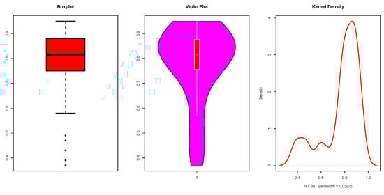
Figure 5. Boxplot, violin, and kernel density plots.

Table 3 provides the estimates, standard errors, and p-values of the parameters of our fitted models for the various conditional quantiles. The estimated parameters were all significant at the $5\%$ level of significance. This is an indication that the LMI and HR have a significant impact on the EAV for all the conditional quantiles. Looking at the signs of the LMI and HR, it is observed that they have a negative impact on the EAV.

Table 3. Estimates of parameters, standard errors, and p-values for some quantiles.

p	Model		${\widehat{\mathit{\rho }}}_0$	${\widehat{\mathit{\rho }}}_1$	${\widehat{\mathit{\rho }}}_2$	$\widehat{\mathit{\beta }}$
0.1	SUGHN	Estimates	1.6257	−0.1656	−0.0643	1.0807
		Standard error	0.2160	0.0422	0.0214	0.1330
		p-value	<$0.0001$	<$0.0001$	0.0026	<$0.0001$
	CUGHN	Estimates	1.7212	−0.1865	−0.0688	1.5740
		Standard error	0.2086	0.0427	0.0203	0.2028
		p-value	<$0.0001$	<$0.0001$	<$0.0001$	<$0.0001$
	TUGHN	Estimates	1.7408	−0.1964	−0.0680	1.7576
		Standard error	0.2180	0.0447	0.0193	0.2181
		p-value	<$0.0001$	<$0.0001$	<$0.0001$	<$0.0001$
	SCUGHN	Estimates	1.6884	−0.1860	−0.0652	1.9640
		Standard error	0.2292	0.0449	0.0198	0.2349
		p-value	<$0.0001$	<$0.0001$	0.0010	<$0.0001$
0.25	SUGHN	Estimates	1.8765	−0.1540	−0.0607	1.0766
		Standard error	0.2038	0.0398	0.0198	0.1327
		p-value	<$0.0001$	0.0001	0.0022	<$0.0001$
	CUGHN	Estimates	1.9474	−0.1760	−0.0652	1.5688
		Standard error	0.1999	0.0411	0.0189	0.2023
		p-value	<$0.0001$	<$0.0001$	0.0006	<$0.0001$
	TUGHN	Estimates	1.9661	−0.1849	−0.0644	1.7500
		Standard error	0.2106	0.0433	0.0180	0.2176
		p-value	<$0.0001$	<$0.0001$	<$0.0001$	<$0.0001$
	SCUGHN	Estimates	1.9274	−0.1737	−0.0615	1.9543
		Standard error	0.2195	0.0431	0.0184	0.2342
		p-value	<$0.0001$	<$0.0001$	0.0008	<$0.0001$
0.5	SUGHN	Estimates	2.2111	−0.1418	−0.0571	1.0714
		Standard error	0.1966	0.0373	0.0183	0.1324
		p-value	<$0.0001$	0.0001	0.0018	<$0.0001$
	CUGHN	Estimates	2.2820	−0.1636	−0.0612	1.5611
		Standard error	0.1967	0.0391	0.0175	0.2016
		p-value	<$0.0001$	<$0.0001$	0.0004	<$0.0001$
	TUGHN	Estimates	2.3123	−0.1706	−0.0603	1.7382
		Standard error	0.2083	0.0415	0.0165	0.2167
		p-value	<$0.0001$	<$0.0001$	0.0003	<$0.0001$
	SCUGHN	Estimates	2.2705	−0.1593	−0.0576	1.9403
		Standard error	0.2140	0.0412	0.0170	0.2330
		p-value	<$0.0001$	0.0001	0.0007	<$0.0001$
0.75	SUGHN	Estimates	2.6239	−0.1302	−0.0540	1.0652
		Standard error	0.2019	0.0349	0.0170	0.1319
		p-value	<$0.0001$	0.0002	0.0015	<$0.0001$
	CUGHN	Estimates	2.7527	−0.1506	−0.0576	1.5494
		Standard error	0.2105	0.0370	0.0161	0.2005
		p-value	<$0.0001$	<$0.0001$	0.0004	<$0.0001$
	TUGHN	Estimates	2.7884	−0.1556	−0.0566	1.7210
		Standard error	0.2216	0.0396	0.0153	0.2151
		p-value	<$0.0001$	<$0.0001$	0.0002	<$0.0001$
	SCUGHN	Estimates	2.7154	−0.1450	−0.0542	1.9211
		Standard error	0.2208	0.0391	0.0158	0.2312
		p-value	<$0.0001$	0.0002	0.0006	<$0.0001$
0.9	SUGHN	Estimates	3.0927	−0.1205	−0.0517	1.0573
		Standard error	0.2249	0.0327	0.0161	0.1314
		p-value	<$0.0001$	0.0002	0.0013	<$0.0001$
	CUGHN	Estimates	3.3459	−0.1390	−0.0547	1.5332
		Standard error	0.2518	0.0350	0.0152	0.1991
		p-value	<$0.0001$	<$0.0001$	0.0003	<$0.0001$
	TUGHN	Estimates	3.3563	−0.1425	−0.0539	1.6997
		Standard error	0.2577	0.0375	0.0145	0.2129
		p-value	<$0.0001$	0.0001	0.0002	<$0.0001$
	SCUGHN	Estimates	3.2286	−0.1328	−0.0517	1.9007
		Standard error	0.2458	0.0369	0.0150	0.2291
		p-value	<$0.0001$	0.0003	0.0006	<$0.0001$

Table 4 presents the model selection criteria for our fitted models, and it can be seen that for all the models, the $0.1$ conditional quantile provided the best fit to the data. As the difference between their AICs and ours is greater than 2, all of our fitted models outperformed the models proposed in [3,7] at the $0.1$ conditional quantile. In addition, comparing the various quantiles, our models outperform the UGHN quantile regression model. The SUGHN quantile regression model is the best for all the conditional quantiles.

Table 4. Statistical criteria.

p	Model	$-2\mathit{\ell }$	AIC	BIC
0.1	SUGHN	−75.7186	−67.7186	−61.1682
	CUGHN	−73.9665	−65.9665	−59.4161
	TUGHN	−73.6949	−65.6949	−59.1445
	SCUGHN	−74.6806	−66.6806	−60.1303
0.25	SUGHN	−75.3022	−67.3022	−60.7519
	CUGHN	−73.5322	−65.5322	−58.9819
	TUGHN	−73.2110	−65.2110	−58.6606
	SCUGHN	−74.1924	−66.1924	−59.6421
0.5	SUGHN	−74.7427	−66.7427	−60.1924
	CUGHN	−72.8930	−64.8930	−58.3426
	TUGHN	−72.4684	−64.4684	−57.918
	SCUGHN	−73.4922	−65.4922	−58.9419
0.75	SUGHN	−74.1041	−66.1041	−59.5537
	CUGHN	−72.0697	−64.0697	−57.5193
	TUGHN	−71.5349	−63.5349	−56.9846
	SCUGHN	−72.6694	−64.6694	−58.1190
0.9	SUGHN	−73.5121	−65.5121	−58.9618
	CUGHN	−71.2425	−63.2425	−56.6921
	TUGHN	−70.6513	−62.6513	−56.1010
	SCUGHN	−71.9129	−63.9129	−57.3625

We perform diagnostic checks on the model residuals to examine how adequate the fitted models are. The probability–probability (P–P) plots of the randomized quantile residuals shown in Figure 6 and Figure 7 suggest that the residuals of the SUGHN, CUGHN, TUGHN, and SCUGHN quantile regression models follow the standard normal distribution as the plots cluster along the diagonal.

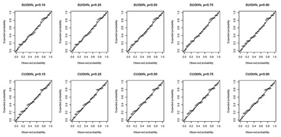
Figure 6. P–P plots of randomized quantile residuals of the SUGHN and CUGHN regression models.

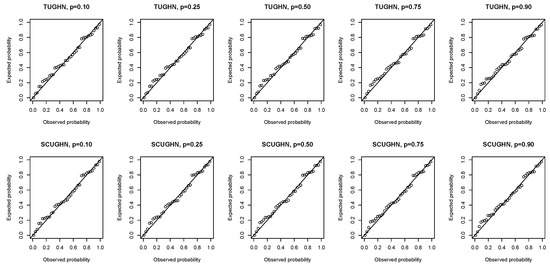
Figure 7. P–P plots of randomized quantile residuals of the TUGHN and SCUGHN regression models.

Further, the randomized quantile residuals are examined using the half-normal plots with the simulated envelope proposed in [30]. Figure 8 and Figure 9 clearly show that the fitted models are adequate since all the observations are inside the simulated envelope.

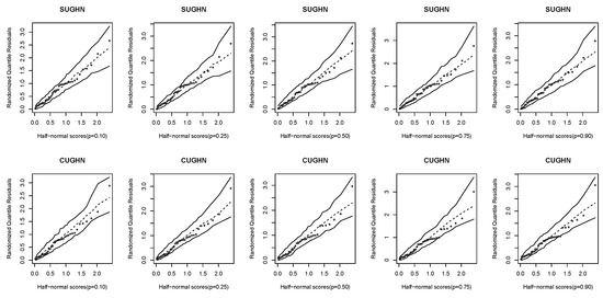
Figure 8. Half-normal plots of randomized quantile residuals of the SUGHN and CUGHN regression models.

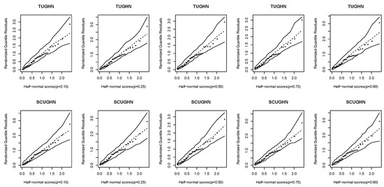
Figure 9. Half-normal plots of randomized quantile residuals of the TUGHN and SCUGHN regression models.

8. Conclusions

In this study, we developed four trigonometric extensions of the UGHN distribution. These are the SUGHN, CUGHN, TUGHN, and SCUGHN distributions. Their PDFs exhibit desirable shapes, such as left-skewed, right-skewed, approximately symmetric, reversed-J, J, and bathtub shapes, making the new distributions suitable candidate models for data with these characteristics. Given the flexibility of the proposed distributions, we developed four quantile regression models for studying the relationship between a response variable and a set of independent variables. The maximum likelihood method was used to estimate the parameters of the regression model, and the Monte Carlo simulation performed showed that the method is able to estimate the parameters well. An empirical illustration of the model using educational data from OECD countries demonstrated that the models provided a good fit, as evidenced by the residual diagnostics. From the application of the model, we observed that the LMI and HR have significant negative effects on the EAV. Thus, to ensure good EAV, issues of LMI and HR need to be addressed with all seriousness.

References

- Ferrari, S.; Cribari-Neto, F. Beta regression for modelling rates and proportions. J. Appl. Stat. 2004, 31, 799–815. [Google Scholar] [CrossRef]
- Mazucheli, J.; Alves, B.; Korkmaz, M.Ç; Leiva, V. Vasicek quantile and mean regression models for bounded data: New formulations, mathematical derivations and numerical applications. Mathematics 2022, 10, 1389. [Google Scholar] [CrossRef]
- Altun, E. The log-weighted exponential regression model: Alternative to the beta regression model. Commun. Stat. Theory Methods 2021, 50, 2306–2321. [Google Scholar] [CrossRef]
- Altun, E.; El-Morshedy, M.; Eliwa, M.S. A new regression model for bounded response variable: An alternative to the beta and unit-Lindley regression models. PLoS ONE 2021, 16, e0245627. [Google Scholar] [CrossRef] [PubMed]
- Altun, E.; Cordeiro, G.M. The unit-improved second-degree Lindley distribution: Inference and regression modeling. Comput. Stat. 2020, 35, 259–279. [Google Scholar] [CrossRef]
- Mazucheli, J.; Menezes, A.F.B.; Chakraborty, S. On the one parameter unit-Lindley distribution and its associated regression model for proportion data. J. Appl. Stat. 2019, 46, 700–714. [Google Scholar] [CrossRef]
- Mazucheli, J.; Korkmaz, M.Ç.; Menezes, A.F.B.; Leiva, V. The unit generalized half-normal quantile regression model: Formulation, estimation, diagnostics and numerical applications. Soft Comput. 2023, 27, 279–295. [Google Scholar] [CrossRef]
- Abubakari, A.G.; Luguterah, A.; Nasiru, S. Unit exponentiated Fréchet distribution: Actuarial measures, quantile regression and applications. J. Indian Soc. Probab. Stat. 2022, 23, 387–424. [Google Scholar] [CrossRef]
- Mustapha, M.H.B.; Nasiru, S. Unit gamma/Gompertz quantile regression with applications to skewed data. Sri Lankan J. Appl. Stat. 2022, 23, 49–73. [Google Scholar] [CrossRef]
- Shekhawat, K.; Sharma, V.K. An extension of J-shaped distribution with application to tissue damage proportions in blood. Sankhya B Indian J. Stat. 2020, 83, 548–574. [Google Scholar] [CrossRef]
- Korkmaz, M.Ç.; Korkmaz, Z.S. The unit log-log distribution: A new unit distribution with alternative quantile regression modeling and educational measurements applications. J. Appl. Stat. 2023, 50, 889–908. [Google Scholar] [CrossRef]
- Ribeiro, T.F.; Pena-Ramírez, F.A.; Guerra, R.R.; Cordeiro, G.M. Another unit Burr XII quantile regression model based on the different reparameterization applied to dropout in Brazilian undergraduate courses. PLoS ONE 2022, 17, e0276695. [Google Scholar] [CrossRef]
- Chesneau, C.; Artault, A. On a comparative study on some trigonometric classes of distributions by the analysis of practical datasets. J. Nonlinear Model. Anal. 2021, 3, 225–262. [Google Scholar]
- Souza, L. New Trigonometric Classes of Probabilistic Distributions. Ph.D. Thesis, Universidade Federal Rural de Pernambuco, Recife, Brazil, 2015. [Google Scholar]
- Korkmaz, M.M.Ç. The unit generalized half normal distribution: A new bounded distribution with inference and application. Sci. Bull.-Univ. Politeh. Bucharest Ser. A 2020, 82, 133–140. [Google Scholar]
- Souza, L.; Junior, W.R.O.; de Brito, C.C.R.; Chesneau, C.; Ferreira, T.A.E.; Soares, L. On the Sin-G class of distributions: Theory, model and application. J. Math. Model. 2019, 7, 357–379. [Google Scholar]
- Souza, L.; Junior, W.R.O.; de Brito, C.C.R.; Chesneau, C.; Ferreira, T.A.E.; Soares, L. General properties for the Cos-G class of distributions with applications. Eurasian Bull. Math. 2019, 2, 63–79. [Google Scholar]
- Souza, L.; Junior, W.R.O.; de Brito, C.C.R.; Chesneau, C.; Ferreira, T.A.E. Tan-G class of trigonometric distributions and its applications. Cubo 2019, 23, 1–20. [Google Scholar] [CrossRef]
- Souza, L.; de Oliveira, W.R.; de Brito, C.C.R.; Chesneau, C.; Fernandes, R.; Ferreira, T.A. Sec-G class of distributions: Properties and applications. Symmetry 2022, 14, 299. [Google Scholar] [CrossRef]
- Ampadu, C.B. The Tan-G family of distributions with illustration to data in the health sciences. Phys. Sci. Biophys. J. 2019, 3, 000125. [Google Scholar]
- Tomy, L.; Satish, G. A review study on trigonometric transformations of statistical distributions. Biom. Biostat. Int. J. 2021, 10, 130–136. [Google Scholar]
- Kumar, D.; Singh, U.; Singh, S.K. A new distribution using sine function—Its application to bladder cancer patients data. J. Stat. Appl. Probab. 2015, 4, 417–427. [Google Scholar]
- Aldahlan, M.A. Sine Fréchet model: Modeling of COVID-19 death cases in Kingdom of Saudi Arabia. Math. Probl. Eng. 2022, 2022, 2039076. [Google Scholar] [CrossRef]
- Ahmadini, A.A.H. Statistical inference of sine inverse Rayleigh distribution. Comput. Syst. Sci. Eng. 2022, 41, 405–414. [Google Scholar]
- Almetwally, E.M.; Meraou, M.A. Application of environmental data with new extension of Nadarajah-Haghighi distribution. Comput. J. Math. Stat. Sci. 2022, 1, 26–41. [Google Scholar] [CrossRef]
- Cooray, K.; Ananda, M. A generalization of the half-normal distribution with applications to lifetime data. Commun. Stat.—Theory Methods 2008, 37, 1323–1337. [Google Scholar] [CrossRef]
- R Core Team. R: A Language and Environment for Statistical Computing; R Foundation for Statistical Computing: Vienna, Austria, 2020; Available online: https://www.R-project.org/ (accessed on 5 October 2022).
- Cox, D.R.; Hinkley, D.V. Theoretical Statistics; Chapman and Hall/CRC: London, UK, 1974. [Google Scholar]
- Dunn, P.K.; Smyth, G.K. Randomized quantile residuals. J. Comput. Graph. Stat. 1996, 5, 236–244. [Google Scholar]
- Atkinson, A.C. Two graphical displays of outlying and influential observations in regression. Biometrika 1981, 68, 13–20. [Google Scholar] [CrossRef]
Disclaimer/Publisher’s Note: The statements, opinions and data contained in all publications are solely those of the individual author(s) and contributor(s) and not of MDPI and/or the editor(s). MDPI and/or the editor(s) disclaim responsibility for any injury to people or property resulting from any ideas, methods, instructions or products referred to in the content. |
© 2023 by the authors. Licensee MDPI, Basel, Switzerland. This article is an open access article distributed under the terms and conditions of the Creative Commons Attribution (CC BY) license (https://creativecommons.org/licenses/by/4.0/).