Fractional–Order Modeling and Control of COVID-19 with Shedding Effect

Abstract

A fractional order COVID-19 model consisting of six compartments in Caputo sense is constructed. The indirect transmission of the virus through susceptible populations by the shedding effect is studied. Equilibrium solutions are calculated, and basic reproduction ratio (that depends both on direct and indirect mode of transmission), existence and uniqueness, as well as stability analysis of the solution of the model, are studied. The paper studies the effect of optimal control policy applied to shedding effect. The control is the observation of standard hygiene practices and chemical disinfectants in public spaces. Numerical simulations are carried out to support the analytic result and to show the significance of the fractional order from the biological viewpoint.

1. Introduction

COVID-19 surfaced in the world at the end of the year 2019. It undermined many sectors such astransport, the economy, education systems, sports, entertainment, etc. The pandemic killed and infected many. The nature and mode of the spread of COVID-19 outbreak are still not completely understood. Researchers are geared towards finding vaccines to curtail the spread of the virus. The idea is to limit the number of new infections and subsequent deaths due to the pandemic. Due to the scarcity of vaccines, many countries in the world adopt non-pharmaceutical measures such as lockdown, airport closures, use of sanitizers and social distancing. There is a great deal of research in the literature with regard to the pandemic, both from a theoretical and practical point of view [1,2,3,4,5,6,7].

It is estimated that 75% of infected individuals recover without showing serious symptoms and many achieve e natural recovery [8]. Throat infection, chest pain, runny nose or nasal congestion, losing smell and taste, vomiting, diarrhea and nausea are some of the symptoms of COVID-19. In most cases, these symptoms appear slowly. It is also believed that elderly people can observe serious complications compared to their younger counterparts. On average, infected individuals spend 7–14 days before showing symptoms [9]. In many cases, it takes 14 days before mild cases recover [10]. The transmission of COVID-19 occurs mostly via either a direct (through contaminated air by tiny droplets and airborne particles containing the virus) or an indirect (through contaminated surfaces) method. The virus is released from the mouth of infected individuals through either sneezing or coughing and is shed into the environment in the form of micro-particles in the air. This shedding effect is of paramount significance in studying COVID-19 transmission. Although diagnostic tests and vaccine treatments are now available to curb the spread of the disease, the use of standard hygiene practices and chemical disinfectants in public places must still be maintained.

Many fields of study such as epidemiology, economics and finance, aeronautical engineering, robotics, etc., use optimal control as an effective mathematical tool to optimize control problems [11]. However, there is little in the literature about the use of an optimal control approach to study COVID-19, since control in a real sense varies with time [12,13,14,15,16,17,18].

Fractional order derivatives and fractional integrals are very important tools that are used in the study of mathematical modeling due to their hereditary properties and ability in memory description. In the last few decades, the fractional differential has been used in mathematical modeling of biological phenomena [19,20]. This is because fractional calculus can explain and process the retention and heritage properties of various materials more accurately than integer-order models [21,22]. Due to the effectiveness of mathematical models in studying infectious diseases, recently many scientists have been investigating mathematical models of the COVID-19 pandemic with fractional order derivatives; they have produced excellent results [23,24]. The Caputo fractional order derivative is based on the exponential kernel and details on its operation and its applications can be found in [25,26,27,28]. Caputo fractional derivative gives less noise when compared with other operators [29]. In this paper, we use Caputo fractional order to model the spread and control of COVID-19 with emphasis on shedding effect.

The main contribution of this paper is to mathematically demonstrate the fact that an uninfected population can become infected by both direct and indirect methods by the exposed or infected class. Infected and exposed individuals can contaminate the environment by shedding pathogens. It is also our aim to show the effect of healthy hygiene practices, i.e., using alcohol-based hand sanitizers and effective chemical disinfectants in public areas in curbing the spread of COVID-19.

This paper is organized as follows: the introduction is given in Section 1, formulation of the model is given in Section 2, analysis of the model is given in Section 3, construction and analysis of the optimal control problem is given in Section 4, numerical simulation is given in Section 5 and finally conclusions are given in Section 6.

2. Definition of Terms

In this section we give definitions of the Caputo derivative as in [30].

Definition 1.

The Caputo fractional left-sided derivative is defined as

$${}_{\ast }{}^{C}D{}_{a+}^{\alpha }\left(f\left(t\right)\right)=\frac{1}{\Gamma \left(n-\alpha \right)}\underset{a}{\overset{t}{{\displaystyle \int }}}{\left(t-\tau \right)}^{n-\alpha -1}\frac{d^n}{d{\tau }^n}\left[f\left(\tau \right)\right]d\tau , t\ge a$$

Caputo fractional right-sided derivative is defined as

$${}_{\ast }{}^{C}D{}_{b-}^{\alpha }\left(f\left(t\right)\right)=\frac{{\left(-1\right)}^n}{\Gamma \left(n-\alpha \right)}\underset{t}{\overset{b}{{\displaystyle \int }}}{\left(\tau -t\right)}^{n-\alpha -1}\frac{d^n}{d{\tau }^n}\left[f\left(\tau \right)\right]d\tau , t\le b.$$

3. Formulation of the Model

We adopted and modified the model in [28]. The transmission of COVID-19 occurs through primary and secondary routes. The primary route is through person–person contact and the secondary route is through contaminated surfaces (shedding effect). While much research on the control of pathogen transmission through the primary route are available in the literature, little considers the secondary route. The control of the transmission through the secondary route involves healthy hygiene practices which include using hand sanitizers, face masks and effective chemical disinfectants in public areas.

The model consists of a system of fractional order differential equation in the Caputo sense with six compartments. The compartments are: $S\left(t\right), E\left(t\right), I\left(t\right), H\left(t\right),R\left(t\right) and V\left(t\right)$ which stands for Susceptible, Exposed, Infected, Hospitalized, and Recovered compartments, respectively. To study the shedding effect, another compartment for contaminated surfaces is added as Virus class V(t).

First, we will consider and analyze the fractional order model in Caputo sense without the optimal control and then in Section 5 we will introduce and analyze the optimal control function.

The model is given below

$$\begin{gathered} {}_0{}^{C}D{}_t^{\alpha }S\left(t\right)={{\rm Y}}^{\alpha }-{\beta }^{\alpha }SI-{\theta }^{\alpha }SV-{\mu }^{\alpha }S, \\ {}_0{}^{C}D{}_t^{\alpha }E\left(t\right)={\beta }^{\alpha }SI+{\theta }^{\alpha }SV-\left({\mu }^{\alpha }+{\gamma }^{\alpha }+{\eta }_1^{\alpha }\right)E, \\ {}_0{}^{C}D{}_t^{\alpha }I={\gamma }^{\alpha }E-\left({\mu }^{\alpha }+{\pi }^{\alpha }+{\xi }_1^{\alpha }+{\eta }_2^{\alpha }\right)I, \\ {}_0{}^{C}D{}_t^{\alpha }H={\pi }^{\alpha }I-\left({\mu }^{\alpha }+{\xi }_2^{\alpha }+{\eta }_3^{\alpha }\right)H, \\ {}_0{}^{C}D{}_t^{\alpha }R\left(t\right)={\eta }_1^{\alpha }E+{\eta }_2^{\alpha }I+{\eta }_3^{\alpha }H-{\mu }^{\alpha }R, \\ {}_0{}^{C}D{}_t^{\alpha }V\left(t\right)=q_1{}^{\alpha }E+q_2{}^{\alpha }I-r^{\alpha }V, \end{gathered}$$

(1)

with the following initial conditions

$$S\left(0\right)=a_1,E\left(0\right)=a_2,I\left(0\right)=a_3,H\left(0\right)=a_4, R\left(0\right)=a_5 and V\left(0\right)=a_6$$

The meaning of the parameters involved in the model is given in

Table 1. Meaning of Parameters.

Parameter	Meaning
${\rm Y}$	Recruitment rate into susceptible class
$\beta$	Transmission rate of COVID-19 from human to human
$\theta$	Transmission rate of COVID-19 from environment to human
μ	Natural death rate
γ	Rate at which exposed individuals move to Infected class
${\eta }_1,{\eta }_2,{\eta }_3$	Natural recovery rate in Exposed, Infected and Hospitalized classes respectively
$\pi$	Rate of hospitalization
${\xi }_1,{\xi }_2$	Rate of COVID-19 caused death in Infected and Hospitalized classes respectively
$q_1,q_2$	Rate of virus shedding from Exposed and Infected classes respectively
r	Rate of sanitization
$0<\alpha \le 1$	Fractional order

below.

4. Analysis of the Model

In this section, some mathematical properties of the model are explored. This consists of positivity and boundedness, computation of Equilibria, basic reproduction number, existence and uniqueness analysis of the solution of the model, and local stability analysis.

4.1. Positivity and Boundedness

To show positivity, considering Equation (1), we have

$$\begin{gathered} {}_0{}^{C}D{}_t^{\alpha }S\left(t\right){|}_{S=0}={{\rm Y}}^{\alpha }>0, \\ {}_0{}^{C}D{}_t^{\alpha }E\left(t\right){|}_{E=0}={\beta }^{\alpha }SI+{\theta }^{\alpha }SV\ge 0, \\ {}_0{}^{C}D{}_t^{\alpha }I\left(t\right){|}_{I=0}={\gamma }^{\alpha }E\ge 0, \\ {}_0{}^{C}D{}_t^{\alpha }H\left(t\right){|}_{H=0}={\pi }^{\alpha }I\ge 0, and \\ {}_0{}^{C}D{}_t^{\alpha }R\left(t\right){|}_{R=0}={\eta }_1^{\alpha }E+{\eta }_2^{\alpha }I+{\eta }_3^{\alpha }H\ge 0. \end{gathered}$$

Therefore, we can observe that the solution of (1) is non-negative.

For the boundedness, we can observe that the overall dynamics of the human population is obtained by adding the first five Equations of (1). Let

$$N\left(t\right)=S\left(t\right)+E\left(t\right)+I\left(t\right)+H\left(t\right)+R\left(t\right)$$

Then,

$${}_0{}^{C}D{}_t^{\alpha }N\left(t\right)={}_0{}^{C}D{}_t^{\alpha }S\left(t\right)+{}_0{}^{C}D{}_t^{\alpha }E\left(t\right)+{}_0{}^{C}D{}_t^{\alpha }I\left(t\right)+{}_0{}^{C}D{}_t^{\alpha }H\left(t\right)+{}_0{}^{C}D{}_t^{\alpha }R\left(t\right),$$

which simplifies to,

$${}_0{}^{C}D{}_t^{\alpha }N\left(t\right)={{\rm Y}}^{\alpha }-{\mu }^{\alpha }N-\left({\xi }_1^{\alpha }I+{\xi }_2^{\alpha }H\right),$$

hence,

$${}_0{}^{C}D{}_t^{\alpha }N\left(t\right)\le {{\rm Y}}^{\alpha }-{\mu }^{\alpha }N.$$

We apply the lap-lace transform method to solve the Gronwall’s like inequality with initial condition $N\left(t_0\right)\ge 0$. We have,

$$\mathcal{L}\left\{{}_0{}^{C}D{}_t^{\alpha }N\left(t\right)+{\mu }^{\alpha }N\right\}\le \mathcal{L}\left\{{{\rm Y}}^{\alpha }\right\}.$$

By linearity of the Laplace transform, we get

$$\mathcal{L}\left\{{}_0{}^{C}D{}_t^{\alpha }N\left(t\right)\}+{\mu }^{\alpha }\mathcal{L}\{N\left(t\right)\right\}\le \mathcal{L}\left\{{{\rm Y}}^{\alpha }\right\},$$

Then we get,

$$S^{\alpha }\mathcal{L}\left\{N\left(t\right)\right\}-{\displaystyle \sum }_{k=0}^{n-1}{S}^{\alpha -k-1}{N}^k\left(t_0\right)+{\mu }^{\alpha }\mathcal{L}\left\{N\left(t\right)\right\}\le \frac{{{\rm Y}}^{\alpha }}{S}.$$

Simplifying, we get

$$\mathcal{L}\left\{N\left(t\right)\right\}\le {{\rm Y}}^{\alpha }\left(\frac{1}{S}-\frac{1}{S}\frac{1}{\left(1+\frac{{\mu }^{\alpha }}{S^{\alpha }}\right)}\right)+{\displaystyle \sum }_{k=0}^{n-1}\frac{1}{S^{k+1}}\frac{1}{\left(1+\frac{{\mu }^{\alpha }}{S^{\alpha }}\right)}{N}^k\left(t_0\right).$$

Using Taylor series expansion, we have

$$\frac{1}{\left(1+\frac{{\mu }^{\alpha }}{S^{\alpha }}\right)}={\displaystyle \sum }_{n=0}^{\infty }{\left(\frac{-{\mu }^{\alpha }}{S^{\alpha }}\right)}^n$$

Therefore,

$$\mathcal{L}\left\{N\left(t\right)\right\}\le {{\rm Y}}^{\alpha }\left(\frac{1}{S}-\frac{1}{S}{\displaystyle \sum }_{n=0}^{\infty }{\left(\frac{-{\mu }^{\alpha }}{S^{\alpha }}\right)}^n\right)+{\displaystyle \sum }_{k=0}^{n-1}\frac{1}{S^{k+1}}{N}^k\left(t_0\right){\displaystyle \sum }_{n=0}^{\infty }{\left(\frac{-{\mu }^{\alpha }}{S^{\alpha }}\right)}^n$$

Taking, Laplace inverse, we get

$$N\left(t\right)\le {{\rm Y}}^{\alpha }-{{\rm Y}}^{\alpha }{\displaystyle \sum }_{n=0}^{\infty }\frac{-{\left({\mu }^{\alpha }{t}^{\alpha }\right)}^n}{\Gamma \left(\alpha n+1\right)}+{\displaystyle \sum }_{k=0}^{n-1}{\displaystyle \sum }_{n=0}^{\infty }\begin{array}{c}\frac{-{\left({\mu }^{\alpha }{t}^{\alpha }\right)}^n}{\Gamma \left(\alpha n+k+1\right)}\\ t^k{N}^k\left(t_0\right).\end{array}$$

Substituting the Mittag-Leffler function, we get

$$N\left(t\right)\le {{\rm Y}}^{\alpha }\left[1-E_1\left(-{\mu }^{\alpha }{t}^{\alpha }\right)\right]+{\displaystyle \sum }_{k=0}^{n-1}{E}_{k+1}\left(-{\mu }^{\alpha }{t}^{\alpha }\right)t^k{N}^k\left(t_0\right).$$

where $E_1\left(-{\mu }^{\alpha }{t}^{\alpha }\right), E_{k+1}\left(-{\mu }^{\alpha }{t}^{\alpha }\right)$ are the series of Mittag-Leffler functions which converge for any argument; hence we say that the solution to the model is bounded.

Thus we define,

$$\begin{array}{r}\omega =\{\left(S\left(t\right), E\left(t\right),I\left(t\right),H\left(t\right),R\left(t\right)\right)\in R_{+}^5:S\left(t\right), E\left(t\right),I\left(t\right),H\left(t\right),R\left(t\right)\\ \le {{\rm Y}}^{\alpha }\left[1-E_1\left(-{\mu }^{\alpha }{t}^{\alpha }\right)\right]+{\displaystyle \sum _{k=0}^{n-1}}{E}_{k+1}\left(-{\mu }^{\alpha }{t}^{\alpha }\right)t^k{N}^k\left(t_0\right)\}\end{array}$$

Hence, all solutions of (1) commencing in $\omega$ stay in $\omega$ for all $t\ge 0$. Positivity of solutions means that the population thrives, while boundedness means that the population growth is restricted naturally due to limited resources.

4.2. Equilibria and Basic Reproduction Number

The equilibrium solutions are obtained by equating the equations in the model to zero and solving the system simultaneously. We obtain two equilibrium solutions; disease free and endemic equilibrium solutions.

• Disease free equilibrium ($E^0$)

  $$E^0=\left\{S_0, E_0,I_0,H_0,R_0,V_0\right\}=\left\{\frac{{{\rm Y}}^{\alpha }}{{\mu }^{\alpha }},0,0,0,0,0\right\}$$
• Endemic equilibrium ($E^1$)

$$E^1=\left\{S_1, E_1,I_1,H_1,R_1,V_1\right\},$$

where,

$$\begin{gathered} S_1=\frac{r^{\alpha }\left({\pi }^{\alpha }+{\eta }_2^{\alpha }+{\mu }^{\alpha }+{\xi }_1^{\alpha }\right)\left({\mu }^{\alpha }+{\eta }_1^{\alpha }+{\gamma }^{\alpha }\right)E_1}{{\beta }^{\alpha }{\gamma }^{\alpha }{r}^{\alpha }+{\theta }^{\alpha }\left(q_1^{\alpha }\left({\pi }^{\alpha }+{\eta }_2^{\alpha }+{\mu }^{\alpha }+{\xi }_1^{\alpha }\right)+q_2^{\alpha }{\gamma }^{\alpha }\right)}, \\ {I}_1=\frac{{\gamma }^{\alpha }{E}_1}{{\pi }^{\alpha }+{\eta }_2^{\alpha }+{\mu }^{\alpha }+{\xi }_1^{\alpha }}, \\ {H}_1=\frac{{\gamma }^{\alpha }{\pi }^{\alpha }{E}_1}{\left({\eta }_3^{\alpha }+{\mu }^{\alpha }+{\xi }_2^{\alpha }\right)\left({\pi }^{\alpha }+{\eta }_2^{\alpha }+{\mu }^{\alpha }+{\xi }_1^{\alpha }\right)}, \\ {R}_1=\frac{1}{{\mu }^{\alpha }}[{\eta }_1^{\alpha }+\frac{{\eta }_3^{\alpha }{\pi }^{\alpha }{\gamma }^{\alpha }}{\left({\eta }_3^{\alpha }+{\mu }^{\alpha }+{\xi }_2^{\alpha }\right)\left({\pi }^{\alpha }+{\eta }_2^{\alpha }+{\mu }^{\alpha }+{\xi }_1^{\alpha }\right)} \\ +\frac{{\eta }_2^{\alpha }{\gamma }^{\alpha }}{{\pi }^{\alpha }+{\eta }_2^{\alpha }+{\mu }^{\alpha }+{\xi }_1^{\alpha }}]E_1, \\ {V}_1=\frac{1}{r^{\alpha }}\left[q_1^{\alpha }+\frac{q_2^{\alpha }{\gamma }^{\alpha }}{{\pi }^{\alpha }+{\eta }_2^{\alpha }+{\mu }^{\alpha }+{\xi }_1^{\alpha }}\right]E_1, \end{gathered}$$

and $E_1$ is defined as

$$\begin{array}{cc}{E}_1=\frac{1}{\left({\mu }^{\alpha }+{\eta }_1^{\alpha }+{\gamma }^{\alpha }\right)}[{{\rm Y}}^{\alpha }\hfill & -\frac{{\mu }^{\alpha }{r}^{\alpha }\left({\pi }^{\alpha }+{\eta }_2^{\alpha }+{\mu }^{\alpha }+{\xi }_1^{\alpha }\right)\left({\mu }^{\alpha }+{\eta }_1^{\alpha }+{\gamma }^{\alpha }\right)}{{\beta }^{\alpha }{\gamma }^{\alpha }{r}^{\alpha }+{\theta }^{\alpha }\left(q_1^{\alpha }\left({\pi }^{\alpha }+{\eta }_2^{\alpha }+{\mu }^{\alpha }+{\xi }_1^{\alpha }\right)+q_2^{\alpha }{\gamma }^{\alpha }\right)}]\end{array}$$

4.3. Computation of Basic Reproduction Ratio

In this section, a threshold quantity called basic reproduction ratio is computed using the method of next generation matrix. Consider the following Equations from (1):

$$\begin{gathered} {}_0{}^{C}D{}_t^{\alpha }E\left(t\right)={\beta }^{\alpha }SI+{\theta }^{\alpha }SV-\left({\mu }^{\alpha }+{\gamma }^{\alpha }+{\eta }_1^{\alpha }\right)E, \\ {}_0{}^{C}D{}_t^{\alpha }I={\gamma }^{\alpha }E-\left({\mu }^{\alpha }+{\pi }^{\alpha }+{\xi }_1^{\alpha }+{\eta }_2^{\alpha }\right)I, \\ {}_0{}^{C}D{}_t^{\alpha }V\left(t\right)=q_{1}E+q_{2}I-rV. \end{gathered}$$

(2)

Let $A_i\left(X\right) and B_i\left(X\right)$ be the rate of appearance of new infection and rate of other transitions in the ith compartment respectively. Then

$$\begin{gathered} A_i\left(X\right)=\left(\begin{array}{c}{\beta }^{\alpha }SI+{\theta }^{\alpha }SV\\ 0\\ 0\end{array}\right), and B_i\left(X\right) \\ =\left(\begin{array}{c}\left({\mu }^{\alpha }+{\gamma }^{\alpha }+{\eta }_1^{\alpha }\right)E\\ -{\gamma }^{\alpha }E+\left({\mu }^{\alpha }+{\pi }^{\alpha }+{\xi }_1^{\alpha }+{\eta }_2^{\alpha }\right)I\\ -q_1{}^{\alpha }E-q_2{}^{\alpha }I+r^{\alpha }V\end{array}\right). \end{gathered}$$

Then Equation (2) can be written as

$$\dot{X}=A_i\left(X\right)-B_i\left(X\right), i=1,2,3.$$

Now, define

$$\begin{gathered} A=\left(\frac{\partial A_i}{\partial x_j}\right)\left(E_0\right)=\left(\begin{array}{ccc}0& \frac{{{\rm Y}}^{\alpha }{\beta }^{\alpha }}{{\mu }^{\alpha }}& \frac{{\theta }^{\alpha }{\beta }^{\alpha }}{{\mu }^{\alpha }}\\ 0& 0& 0\\ 0& 0& 0\end{array}\right), and \\ B=\left(\frac{\partial B_i}{\partial x_j}\right)\left(E_0\right)=\left(\begin{array}{ccc}{\mu }^{\alpha }+{\gamma }^{\alpha }+{\eta }_1^{\alpha }& 0& 0\\ -{\gamma }^{\alpha }E& {\mu }^{\alpha }+{\pi }^{\alpha }+{\xi }_1^{\alpha }+{\eta }_2^{\alpha }& 0\\ -q_1{}^{\alpha }& -q_2{}^{\alpha }& r^{\alpha }\end{array}\right). \end{gathered}$$

The basic reproduction ratio, which is the spectral radius of the matrix $A{B}^{-1},$ defined as $\rho \left(A{B}^{-1}\right),$ is calculated as

$$R_0=R_1+R_2+R_3,$$

where

$$\begin{gathered} R_1=\frac{{{\rm Y}}^{\alpha }{\beta }^{\alpha }{\gamma }^{\alpha }}{{\mu }^{\alpha }\left({\mu }^{\alpha }+{\pi }^{\alpha }+{\xi }_1^{\alpha }+{\eta }_2^{\alpha }\right)\left({\mu }^{\alpha }+{\gamma }^{\alpha }+{\eta }_1^{\alpha }\right)}, \\ R_2=\frac{{{\rm Y}}^{\alpha }{\theta }^{\alpha }{q}_1{}^{\alpha }}{{\mu }^{\alpha }{r}^{\alpha }\left({\mu }^{\alpha }+{\gamma }^{\alpha }+{\eta }_1^{\alpha }\right)}, and \\ {R}_3=\frac{{\theta }^{\alpha }{{\rm Y}}^{\alpha }{q}_2{}^{\alpha }{\gamma }^{\alpha }}{{\mu }^{\alpha }{r}^{\alpha }\left({\mu }^{\alpha }+{\pi }^{\alpha }+{\xi }_1^{\alpha }+{\eta }_2^{\alpha }\right)\left({\mu }^{\alpha }+{\gamma }^{\alpha }+{\eta }_1^{\alpha }\right)} \end{gathered}$$

where $R_1,R_2 and R_3$ are related with the endowment of direct human-to-human contact routes, exposed-to-environment and infected-to-environment, respectively.

4.4. Existence and Uniqueness of Solution of the Model

Consider the system

$$\begin{gathered} S\left(t\right)-S\left(0\right)={}_0{}^{C}D{}_t^{\alpha }S\left(t\right)\left\{{{\rm Y}}^{\alpha }-{\beta }^{\alpha }SI-{\theta }^{\alpha }SV-{\mu }^{\alpha }S\right\}, \\ E\left(t\right)-E\left(0\right)={}_0{}^{C}D{}_t^{\alpha }E\left(t\right)\left\{{\beta }^{\alpha }SI+{\theta }^{\alpha }SV-\left({\mu }^{\alpha }+{\gamma }^{\alpha }+{\eta }_1^{\alpha }\right)E\right\}, \\ I\left(t\right)-I\left(0\right)={}_0{}^{C}D{}_t^{\alpha }I\left\{{\gamma }^{\alpha }E-\left({\mu }^{\alpha }+{\pi }^{\alpha }+{\xi }_1^{\alpha }+{\eta }_2^{\alpha }\right)I\right\}, \\ H\left(t\right)-H\left(0\right)={}_0{}^{C}D{}_t^{\alpha }H\left\{{\pi }^{\alpha }I-\left({\mu }^{\alpha }+{\xi }_2^{\alpha }+{\eta }_3^{\alpha }\right)H\right\}, \\ R\left(t\right)-R\left(0\right)={}_0{}^{C}D{}_t^{\alpha }R\left(t\right)\left\{{\eta }_1^{\alpha }E+{\eta }_2^{\alpha }I+{\eta }_3^{\alpha }H-{\mu }^{\alpha }R\right\}, \\ V\left(t\right)-V\left(0\right)={}_0{}^{C}D{}_t^{\alpha }V\left(t\right)\left\{q_1{}^{\alpha }E+q_2{}^{\alpha }I-r^{\alpha }V\right\}, \end{gathered}$$

and

$$\begin{gathered} S\left(t\right)-S\left(0\right)=M\left(\alpha \right){{\displaystyle \int }}_0^1{\left(t-\tau \right)}^{-\alpha }{F}_1\left(t,S\right)d\tau , \\ E\left(t\right)-E\left(0\right)=M\left(\alpha \right){{\displaystyle \int }}_0^1{\left(t-\tau \right)}^{-\alpha }{F}_2\left(t,E\right)d\tau , \\ I\left(t\right)-I\left(0\right)=M\left(\alpha \right){{\displaystyle \int }}_0^1{\left(t-\tau \right)}^{-\alpha }{F}_3\left(t,I\right)d\tau , \\ H\left(t\right)-H\left(0\right)=M\left(\alpha \right){{\displaystyle \int }}_0^1{\left(t-\tau \right)}^{-\alpha }{F}_4\left(t,H\right)d\tau , \\ R\left(t\right)-R\left(0\right)=M\left(\alpha \right){{\displaystyle \int }}_0^1{\left(t-\tau \right)}^{-\alpha }{F}_5\left(t,R\right)d\tau , \\ V\left(t\right)-V\left(0\right)=M\left(\alpha \right){{\displaystyle \int }}_0^1{\left(t-\tau \right)}^{-\alpha }{F}_6\left(t,V\right)d\tau , \end{gathered}$$

where

$$\begin{gathered} {}_0{}^{C}D{}_t^{\alpha }S\left(t\right)=F_1\left(t,S\right), \\ {}_0{}^{C}D{}_t^{\alpha }E\left(t\right)=F_2\left(t,E\right), \\ {}_0{}^{C}D{}_t^{\alpha }I\left(t\right)=F_3\left(t,I\right), \\ {}_0{}^{C}D{}_t^{\alpha }H\left(t\right)=F_4\left(t,H\right), \\ {}_0{}^{C}D{}_t^{\alpha }R\left(t\right)=F_5\left(t,R\right), \\ {}_0{}^{C}D{}_t^{\alpha }V\left(t\right)=F_6\left(t,V\right). \end{gathered}$$

Now, we can easily show that $F_1,\dots , F_6$ satisfy Lipschitz continuity using the following theorem

$$0\le {\beta }^{\alpha }{k}_1+{\theta }^{\alpha }{k}_2+{\mu }^{\alpha }<1,$$

This is a contraction.

Proof. 

$$\begin{array}{c}\Vert F_1\left(t,S\right)-F_1\left(t,S_1\right)\Vert \\ =\Vert {{\rm Y}}^{\alpha }-{\beta }^{\alpha }S\left(t\right)I\left(t\right)-{\theta }^{\alpha }S\left(t\right)V\left(t\right)-{\mu }^{\alpha }S\left(t\right)-{{\rm Y}}^{\alpha }\\ +{\beta }^{\alpha }{S}_1\left(t\right)I\left(t\right)+{\theta }^{\alpha }{S}_1\left(t\right)V\left(t\right)+{\mu }^{\alpha }{S}_1\left(t\right)\Vert \\ =\Vert -{\beta }^{\alpha }I\left(t\right)\left(S\left(t\right)-S_1\left(t\right)\right)-{\theta }^{\alpha }V\left(t\right)\left(S\left(t\right)-S_1\left(t\right)\right)-{\mu }^{\alpha }\left(S\left(t\right)-S_1\left(t\right)\right)\Vert \\ \le {\beta }^{\alpha }\Vert I\left(t\right)\Vert \Vert S\left(t\right)-S_1\left(t\right)\Vert +{\theta }^{\alpha }V\left(t\right)\Vert S\left(t\right)-S_1\left(t\right)\Vert +{\mu }^{\alpha }\Vert S\left(t\right)-S_1\left(t\right)\Vert \\ \le \left({\beta }^{\alpha }{k}_1+{\theta }^{\alpha }{k}_2+{\mu }^{\alpha }\right)\Vert S\left(t\right)-S_1\left(t\right)\Vert \\ \le L_1\Vert S\left(t\right)-S_1\left(t\right)\Vert ,\end{array}$$

where $L_1={\beta }^{\alpha }{k}_1+{\theta }^{\alpha }{k}_2+{\mu }^{\alpha } , k_1\ge \Vert I\left(t\right)\Vert and k_2\ge \Vert V\left(t\right)\Vert .$□

Similarly, we find the remaining Lipschitz constants $L_2,\dots , L_6$ show the Lischitz continuity and contraction of $F_2,\dots , F_6.$

Recursively, let

$$\begin{array}{ll}{p}_{1n}\left(t\right)& =S_n\left(t\right)-S_{n-1}\left(t\right)\\ & =\frac{2\left(1-\alpha \right)}{\left(2-\alpha \right)M\left(\alpha \right)}\left(F_1\left(t,S_{n-1}\right)-F_1\left(t,S_{n-2}\right)\right)\\ & +\frac{2\alpha }{\left(2-\alpha \right)M\left(\alpha \right)}\underset{0}{\overset{t}{{\displaystyle \int }}}\left(F_1\left(\vartheta ,S_{n-1}\right)-F_1\left(\vartheta ,S_{n-2}\right)\right)d\vartheta ,\end{array}$$

$$\begin{array}{ll}{p}_{2n}\left(t\right)& =E_n\left(t\right)-E_{n-1}\left(t\right)\\ & =\frac{2\left(1-\alpha \right)}{\left(2-\alpha \right)M\left(\alpha \right)}\left(F_2\left(t,E_{n-1}\right)-F_2\left(t,E_{n-2}\right)\right)\\ & +\frac{2\alpha }{\left(2-\alpha \right)M\left(\alpha \right)}\underset{0}{\overset{t}{{\displaystyle \int }}}\left(F_2\left(\vartheta ,E_{n-1}\right)-F_2\left(\vartheta ,E_{n-2}\right)\right)d\vartheta ,\end{array}$$

$$\begin{array}{ll}{p}_{3n}\left(t\right)& =I_n\left(t\right)-I_{n-1}\left(t\right)\\ & =\frac{2\left(1-\alpha \right)}{\left(2-\alpha \right)M\left(\alpha \right)}\left(F_3\left(t,I_{n-1}\right)-F_3\left(t,I_{n-2}\right)\right)\\ & +\frac{2\alpha }{\left(2-\alpha \right)M\left(\alpha \right)}\underset{0}{\overset{t}{{\displaystyle \int }}}\left(F_3\left(\vartheta ,I_{n-1}\right)-F_3\left(\vartheta ,I_{n-2}\right)\right)d\vartheta ,\end{array}$$

$$\begin{array}{ll}{p}_{4n}\left(t\right)& =H_n\left(t\right)-H_{n-1}\left(t\right)\\ & =\frac{2\left(1-\alpha \right)}{\left(2-\alpha \right)M\left(\alpha \right)}\left(F_4\left(t,H_{n-1}\right)-F_4\left(t,H_{n-2}\right)\right)\\ & +\frac{2\alpha }{\left(2-\alpha \right)M\left(\alpha \right)}\underset{0}{\overset{t}{{\displaystyle \int }}}\left(F_4\left(\vartheta ,H_{n-1}\right)-F_4\left(\vartheta ,H_{n-2}\right)\right)d\vartheta ,\end{array}$$

$$\begin{array}{ll}{p}_{5n}\left(t\right)& =R_n\left(t\right)-R_{n-1}\left(t\right)\\ & =\frac{2\left(1-\alpha \right)}{\left(2-\alpha \right)M\left(\alpha \right)}\left(F_5\left(t,R_{n-1}\right)-F_5\left(t,R_{n-2}\right)\right)\\ & +\frac{2\alpha }{\left(2-\alpha \right)M\left(\alpha \right)}\underset{0}{\overset{t}{{\displaystyle \int }}}\left(F_5\left(\vartheta ,R_{n-1}\right)-F_5\left(\vartheta ,R_{n-2}\right)\right)d\vartheta ,\end{array}$$

$$\begin{array}{ll}{p}_{6n}\left(t\right)& =V_n\left(t\right)-V_{n-1}\left(t\right)\\ & =\frac{2\left(1-\alpha \right)}{\left(2-\alpha \right)M\left(\alpha \right)}\left(F_6\left(t,V_{n-1}\right)-F_6\left(t,V_{n-2}\right)\right)\\ & +\frac{2\alpha }{\left(2-\alpha \right)M\left(\alpha \right)}\underset{0}{\overset{t}{{\displaystyle \int }}}\left(F_6\left(\vartheta ,V_{n-1}\right)-F_5\left(\vartheta ,V_{n-2}\right)\right)d\vartheta ,\end{array}$$

with initial conditions

$$S_0\left(t\right)=S\left(0\right),E_0\left(t\right)=E\left(0\right),I_0\left(t\right)=I\left(0\right),H_0\left(0\right)=H\left(0\right), R_0\left(0\right)=R\left(0\right) and V_0\left(0\right)=V\left(0\right)$$

Consider $q_{1n}$ and take the norm, we have

$$\begin{array}{ll}\Vert q_{1n}\left(t\right)\Vert & =\Vert S_n\left(t\right)-S_{n-1}\left(t\right)\Vert \\ & =\Vert \frac{2\left(1-\alpha \right)}{\left(2-\alpha \right)M\left(\alpha \right)}\left(F_1\left(t,S_{n-1}\right)-F_1\left(t,S_{n-2}\right)\right)\\ & +\frac{2\alpha }{\left(2-\alpha \right)M\left(\alpha \right)}\underset{0}{\overset{t}{{\displaystyle \int }}}\left(F_1\left(\vartheta ,S_{n-1}\right)-F_1\left(\vartheta ,S_{n-2}\right)\right)d\vartheta \Vert \end{array}$$

Applying triangular inequality, we have

$$\begin{array}{ll}\Vert p_{1n}\left(t\right)\Vert & =\Vert S_n\left(t\right)-S_{n-1}\left(t\right)\Vert \\ & =\frac{2\left(1-\alpha \right)}{\left(2-\alpha \right)M\left(\alpha \right)}\Vert F_1\left(t,S_{n-1}\right)-F_1\left(t,S_{n-2}\right)\Vert \\ & +\frac{2\alpha }{\left(2-\alpha \right)M\left(\alpha \right)}\Vert \underset{0}{\overset{t}{{\displaystyle \int }}}\left(F_1\left(\vartheta ,S_{n-1}\right)-F_1\left(\vartheta ,S_{n-2}\right)\right)d\vartheta \Vert \\ & \le \frac{2\left(1-\alpha \right)}{\left(2-\alpha \right)M\left(\alpha \right)}{L}_1\Vert S_n-S_{n-1}\Vert \\ & +\frac{2\alpha }{\left(2-\alpha \right)M\left(\alpha \right)}{L}_1\underset{0}{\overset{t}{{\displaystyle \int }}}\Vert S_n-S_{n-1}\Vert d\vartheta .\end{array}$$

This implies

$$\begin{array}{c}\Vert p_{1n}\left(t\right)\Vert \le \frac{2\left(1-\alpha \right)}{\left(2-\alpha \right)M\left(\alpha \right)}{L}_1\Vert p_{1n-1}\left(t\right)\Vert \\ +\frac{2\alpha }{\left(2-\alpha \right)M\left(\alpha \right)}{L}_1\underset{0}{\overset{t}{{\displaystyle \int }}}\Vert p_{1n-1}\left(t\right)\Vert d\vartheta .\end{array}$$

In the same way,

$$\begin{gathered} \Vert p_{2n}\left(t\right)\Vert \le \frac{2\left(1-\alpha \right)}{\left(2-\alpha \right)M\left(\alpha \right)}{L}_2\Vert p_{2n-1}\left(t\right)\Vert +\frac{2\alpha }{\left(2-\alpha \right)M\left(\alpha \right)}{L}_2\underset{0}{\overset{t}{{\displaystyle \int }}}\Vert p_{2n-1}\left(t\right)\Vert d\vartheta , \\ \Vert p_{3n}\left(t\right)\Vert \le \frac{2\left(1-\alpha \right)}{\left(2-\alpha \right)M\left(\alpha \right)}{L}_3\Vert p_{3n-1}\left(t\right)\Vert +\frac{2\alpha }{\left(2-\alpha \right)M\left(\alpha \right)}{L}_3\underset{0}{\overset{t}{{\displaystyle \int }}}\Vert p_{3n-1}\left(t\right)\Vert d\vartheta , \\ \Vert p_{4n}\left(t\right)\Vert \le \frac{2\left(1-\alpha \right)}{\left(2-\alpha \right)M\left(\alpha \right)}{L}_4\Vert p_{4n-1}\left(t\right)\Vert +\frac{2\alpha }{\left(2-\alpha \right)M\left(\alpha \right)}{L}_4\underset{0}{\overset{t}{{\displaystyle \int }}}\Vert p_{4n-1}\left(t\right)\Vert d\vartheta , \\ \Vert p_{5n}\left(t\right)\Vert \le \frac{2\left(1-\alpha \right)}{\left(2-\alpha \right)M\left(\alpha \right)}{L}_5\Vert p_{5n-1}\left(t\right)\Vert +\frac{2\alpha }{\left(2-\alpha \right)M\left(\alpha \right)}{L}_5\underset{0}{\overset{t}{{\displaystyle \int }}}\Vert p_{5n-1}\left(t\right)\Vert d\vartheta , \\ \Vert p_{6n}\left(t\right)\Vert \le \frac{2\left(1-\alpha \right)}{\left(2-\alpha \right)M\left(\alpha \right)}{L}_6\Vert p_{6n-1}\left(t\right)\Vert +\frac{2\alpha }{\left(2-\alpha \right)M\left(\alpha \right)}{L}_6\underset{0}{\overset{t}{{\displaystyle \int }}}\Vert p_{6n-1}\left(t\right)\Vert d\vartheta . \end{gathered}$$

Hence, we have

$$\begin{gathered} S_n\left(t\right)={\displaystyle \sum }_{i=1}^n{p}_{1i}\left(t\right), \\ {E}_n\left(t\right)={\displaystyle \sum }_{i=1}^n{p}_{2i}\left(t\right), \\ {I}_n\left(t\right)={\displaystyle \sum }_{i=1}^n{p}_{3i}\left(t\right), \\ {H}_n\left(t\right)={\displaystyle \sum }_{i=1}^n{p}_{4i}\left(t\right), \\ {R}_n\left(t\right)={\displaystyle \sum }_{i=1}^n{p}_{5i}\left(t\right), \\ {V}_n\left(t\right)={\displaystyle \sum }_{i=1}^n{p}_{6i}\left(t\right). \end{gathered}$$

The following theorem gives the condition for the existence of the solution:

Theorem 1.

The solution exists if$t_1$exists, such that the following inequality is true,

$$\frac{2\left(1-\alpha \right)}{\left(2-\alpha \right)M\left(\alpha \right)}{L}_i+\frac{2\alpha t_1}{\left(2-\alpha \right)M\left(\alpha \right)}{L}_i<1, i=1, \dots , 6$$

Proof. 

Recursively, we have

$$\begin{gathered} \Vert p_{1n}\left(t\right)\Vert \le \Vert S_n\left(0\right)\Vert {\left[\frac{2\left(1-\alpha \right)}{\left(2-\alpha \right)M\left(\alpha \right)}{L}_1+\frac{2\alpha }{\left(2-\alpha \right)M\left(\alpha \right)}{L}_1\right]}^n, \\ \Vert p_{2n}\left(t\right)\Vert \le \Vert E_n\left(0\right)\Vert {\left[\frac{2\left(1-\alpha \right)}{\left(2-\alpha \right)M\left(\alpha \right)}{L}_2+\frac{2\alpha }{\left(2-\alpha \right)M\left(\alpha \right)}{L}_2\right]}^n, \\ \Vert p_{3n}\left(t\right)\Vert \le \Vert I_n\left(0\right)\Vert {\left[\frac{2\left(1-\alpha \right)}{\left(2-\alpha \right)M\left(\alpha \right)}{L}_3+\frac{2\alpha }{\left(2-\alpha \right)M\left(\alpha \right)}{L}_3\right]}^n, \\ \Vert p_{4n}\left(t\right)\Vert \le \Vert H_n\left(0\right)\Vert {\left[\frac{2\left(1-\alpha \right)}{\left(2-\alpha \right)M\left(\alpha \right)}{L}_4+\frac{2\alpha }{\left(2-\alpha \right)M\left(\alpha \right)}{L}_4\right]}^n, \\ \Vert p_{5n}\left(t\right)\Vert \le \Vert R_n\left(0\right)\Vert {\left[\frac{2\left(1-\alpha \right)}{\left(2-\alpha \right)M\left(\alpha \right)}{L}_5+\frac{2\alpha }{\left(2-\alpha \right)M\left(\alpha \right)}{L}_5\right]}^n, \\ \Vert p_{6n}\left(t\right)\Vert \le \Vert V_n\left(0\right)\Vert {\left[\frac{2\left(1-\alpha \right)}{\left(2-\alpha \right)M\left(\alpha \right)}{L}_6+\frac{2\alpha }{\left(2-\alpha \right)M\left(\alpha \right)}{L}_6\right]}^n \end{gathered}$$

□

Hence solutions exist and are continuous. To show that the functions above construct the solutions, consider

$$\begin{gathered} S\left(t\right)-S\left(0\right)=S_n\left(t\right)-M_{1_n}\left(t\right), \\ E\left(t\right)-E\left(0\right)=E_n\left(t\right)-M_{2_n}\left(t\right), \\ I\left(t\right)-I\left(0\right)=I_n\left(t\right)-M_{3_n}\left(t\right), \\ H\left(t\right)-H\left(0\right)=H_n\left(t\right)-M_{4_n}\left(t\right), \\ R\left(t\right)-R\left(0\right)=R_n\left(t\right)-M_{5_n}\left(t\right). \\ V\left(t\right)-V\left(0\right)=V_n\left(t\right)-M_{6_n}\left(t\right). \end{gathered}$$

Hence,

$$\begin{gathered} \Vert M_{1_n}\left(t\right)\Vert =\Vert \frac{2\left(1-\alpha \right)}{\left(2-\alpha \right)M\left(\alpha \right)}\left(F_1\left(t,S_{n-1}\right)-F_1\left(t,S_{n-2}\right)\right)+\frac{2\alpha }{\left(2-\alpha \right)M\left(\alpha \right)}\underset{0}{\overset{t}{{\displaystyle \int }}}\left(F_1\left(\vartheta ,S_{n-1}\right)-F_1\left(\vartheta ,S_{n-2}\right)\right)d\vartheta \Vert \\ \le \frac{2\left(1-\alpha \right)}{\left(2-\alpha \right)M\left(\alpha \right)}\Vert F_1\left(t,S_{n-1}\right)-F_1\left(t,S_{n-2}\right)\Vert +\frac{2\alpha }{\left(2-\alpha \right)M\left(\alpha \right)}\Vert \underset{0}{\overset{t}{{\displaystyle \int }}}\left(F_1\left(\vartheta ,S_{n-1}\right)-F_1\left(\vartheta ,S_{n-2}\right)\right)d\vartheta \Vert \\ \le \frac{2\left(1-\alpha \right)}{\left(2-\alpha \right)M\left(\alpha \right)}{L}_1\Vert S-S_{n-1}\Vert +\frac{2\alpha }{\left(2-\alpha \right)M\left(\alpha \right)}{L}_1\Vert S-S_{n-1}\Vert t. \end{gathered}$$

Carrying out the procedure, we get

$$\Vert M_{1_n}\left(t\right)\Vert \le {\left[\frac{2\left(1-\alpha \right)}{\left(2-\alpha \right)M\left(\alpha \right)}+\frac{2\alpha t}{\left(2-\alpha \right)M\left(\alpha \right)}\right]}^{n+1}{L}_1{}^{n+1}h.$$

At $t=t_1,$ we get

$$\Vert M_{1_n}\left(t\right)\Vert \le {\left[\frac{2\left(1-\alpha \right)}{\left(2-\alpha \right)M\left(\alpha \right)}+\frac{2\alpha t_1}{\left(2-\alpha \right)M\left(\alpha \right)}\right]}^{n+1}{L}_1{}^{n+1}h$$

Taking limit as $n\to \infty ,$ we get

$$\Vert M_{1_n}\left(t\right)\Vert \to 0.$$

Similarly, we have

$$\Vert M_{2_n}\left(t\right)\Vert ,\Vert M_{3_n}\left(t\right)\Vert ,\Vert M_{4_n}\left(t\right)\Vert ,\Vert M_{5_n}\left(t\right)\Vert ,\Vert M_{6_n}\left(t\right)\Vert \to 0.$$

To show uniqueness, assume we have some other solutions, $S^1\left(t\right),E^1\left(t\right),I^1\left(t\right), H^1\left(t\right), R^1\left(t\right), \mathrm{and} V^1\left(t\right),$ then

$$\Vert S\left(t\right)-S^1\left(t\right)\Vert \left(1-\frac{2\left(1-\alpha \right)}{\left(2-\alpha \right)M\left(\alpha \right)}{L}_1-\frac{2\alpha t}{\left(2-\alpha \right)M\left(\alpha \right)}{L}_1\right)\le 0.$$

The completion of the proof is given by the following theorem.

Theorem 2.

If

$$\left(1-\frac{2\left(1-\alpha \right)}{\left(2-\alpha \right)M\left(\alpha \right)}{L}_1-\frac{2\alpha t}{\left(2-\alpha \right)M\left(\alpha \right)}{L}_1\right)>0,$$

then the solution is unique.

Proof. 

Consider

$$\Vert S\left(t\right)-S^1\left(t\right)\Vert \left(1-\frac{2\left(1-\alpha \right)}{\left(2-\alpha \right)M\left(\alpha \right)}{L}_1-\frac{2\alpha t}{\left(2-\alpha \right)M\left(\alpha \right)}{L}_1\right)\le 0$$

Since,

$$\left(1-\frac{2\left(1-\alpha \right)}{\left(2-\alpha \right)M\left(\alpha \right)}{L}_1-\frac{2\alpha t}{\left(2-\alpha \right)M\left(\alpha \right)}{L}_1\right)>0,$$

Then

$$\Vert S\left(t\right)-S^1\left(t\right)\Vert =0$$

Hence,

$$S\left(t\right)=S^1\left(t\right)$$

□

This is true for the remaining solutions.

4.5. Stability Analysis of the Equilibria

Here, we show the local stability of Disease-free equilibrium ($E^0$) and Endemic equilibrium ($E^1$) respectively. For details see [31,32].

Consider the Jacobian matrix obtained from (1), we have

$$J=\left[\begin{array}{ccccc}-{\beta }^{\alpha }I-{\theta }^{\alpha }V-{\mu }^{\alpha }& 0& -{\beta }^{\alpha }S& 0& -{\theta }^{\alpha }S\\ {\beta }^{\alpha }I+{\theta }^{\alpha }V& -\left({\mu }^{\alpha }+{\gamma }^{\alpha }+{\eta }_1^{\alpha }\right)& {\beta }^{\alpha }S& 0& {\theta }^{\alpha }S\\ 0& {\gamma }^{\alpha }& -\left({\mu }^{\alpha }+{\pi }^{\alpha }+{\xi }_1^{\alpha }+{\eta }_2^{\alpha }\right)& 0& 0\\ 0& 0& {\pi }^{\alpha }& -\left({\mu }^{\alpha }+{\xi }_2^{\alpha }+{\eta }_3^{\alpha }\right)& 0\\ 0& q_1^{\alpha }& q_2^{\alpha }& 0& -r^{\alpha }\end{array}\right].$$

(3)

Theorem 3.

Disease-free equilibrium ($E^0$) is locally asymptotically stable when$R_0<1$.

Proof. 

Consider (3) at ($E^0$), we have

$$J\left(E^0\right)=\left[\begin{array}{ccccc}-{\mu }^{\alpha }& 0& -{\beta }^{\alpha }{S}_0& 0& -{\theta }^{\alpha }{S}_0\\ 0& -\left({\mu }^{\alpha }+{\gamma }^{\alpha }+{\eta }_1^{\alpha }\right)& {\beta }^{\alpha }{S}_0& 0& {\theta }^{\alpha }{S}_0\\ 0& {\gamma }^{\alpha }& -\left({\mu }^{\alpha }+{\pi }^{\alpha }+{\xi }_1^{\alpha }+{\eta }_2^{\alpha }\right)& 0& 0\\ 0& 0& {\pi }^{\alpha }& -\left({\mu }^{\alpha }+{\xi }_2^{\alpha }+{\eta }_3^{\alpha }\right)& 0\\ 0& q_1^{\alpha }& q_2^{\alpha }& 0& -r^{\alpha }\end{array}\right].$$

□

The Eigen–values are

$${\lambda }_1=-{\mu }^{\alpha }, {\lambda }_2=-\left({\mu }^{\alpha }+{\eta }_3^{\alpha }+{\xi }_2^{\alpha }\right),$$

${\lambda }_3,{\lambda }_{4 }and {\lambda }_5$ can be found by solving the polynomial equation, $\begin{array}{ll}{\lambda }^3+{\lambda }^2[({\mu }^{\alpha }+& {\pi }^{\alpha }+{\xi }_1^{\alpha }+{\eta }_2^{\alpha })+({\mu }^{\alpha }+{\gamma }^{\alpha }+{\eta }_1^{\alpha })+r^{\alpha }]\\ & +\lambda [({\mu }^{\alpha }+{\pi }^{\alpha }+{\xi }_1^{\alpha }+{\eta }_2^{\alpha })({\mu }^{\alpha }+{\gamma }^{\alpha }+{\eta }_1^{\alpha })+({\mu }^{\alpha }+{\pi }^{\alpha }+{\xi }_1^{\alpha }+{\eta }_2^{\alpha })r^{\alpha }\\ & +({\mu }^{\alpha }+{\gamma }^{\alpha }+{\eta }_1^{\alpha })r^{\alpha }-q_1^{\alpha }{\theta }^{\alpha }{S}_0-{\gamma }^{\alpha }{\beta }^{\alpha }{S}_0]\\ & +[({\mu }^{\alpha }+{\pi }^{\alpha }+{\xi }_1^{\alpha }+{\eta }_2^{\alpha })({\mu }^{\alpha }+{\gamma }^{\alpha }+{\eta }_1^{\alpha })r^{\alpha }\\ & -[({\mu }^{\alpha }+{\pi }^{\alpha }+{\xi }_1^{\alpha }+{\eta }_2^{\alpha })q_1^{\alpha }{\theta }^{\alpha }{S}_0+{\gamma }^{\alpha }{\beta }^{\alpha }{S}_0{r}^{\alpha }+{\gamma }^{\alpha }{\beta }^{\alpha }{S}_0{q}_1^{\alpha }{\theta }^{\alpha }{S}_0]]=0.\end{array}$

By Routh-Hurwitz criterion, Eigen-values of $f\left(s\right)=a_0{s}^3+a_1{s}^2+a_{2}s+a_3,$ are all negative if $a_1>0, a_3>0, and a_1{a}_2>a_3.$

In this case,

$$\begin{gathered} a_1=\left({\mu }^{\alpha }+{\pi }^{\alpha }+{\xi }_1^{\alpha }+{\eta }_2^{\alpha }\right)+\left({\mu }^{\alpha }+{\gamma }^{\alpha }+{\eta }_1^{\alpha }\right)+r^{\alpha }>0, \\ {a}_3=\left({\mu }^{\alpha }+{\pi }^{\alpha }+{\xi }_1^{\alpha }+{\eta }_2^{\alpha }\right)\left({\mu }^{\alpha }+{\gamma }^{\alpha }+{\eta }_1^{\alpha }\right)r^{\alpha } \\ -[\left({\mu }^{\alpha }+{\pi }^{\alpha }+{\xi }_1^{\alpha }+{\eta }_2^{\alpha }\right)q_1^{\alpha }{\theta }^{\alpha }{S}_0+{\gamma }^{\alpha }{\beta }^{\alpha }{S}_0{r}^{\alpha } \\ +{\gamma }^{\alpha }{\beta }^{\alpha }{S}_0{q}_1^{\alpha }{\theta }^{\alpha }{S}_0]>0, \end{gathered}$$

if

$$\begin{gathered} \frac{\left[\left({\mu }^{\alpha }+{\pi }^{\alpha }+{\xi }_1^{\alpha }+{\eta }_2^{\alpha }\right)q_1^{\alpha }{\theta }^{\alpha }{S}_0+{\gamma }^{\alpha }{\beta }^{\alpha }{S}_0{r}^{\alpha }+{\gamma }^{\alpha }{\beta }^{\alpha }{S}_0{q}_1^{\alpha }{\theta }^{\alpha }{S}_0\right]}{\left({\mu }^{\alpha }+{\pi }^{\alpha }+{\xi }_1^{\alpha }+{\eta }_2^{\alpha }\right)\left({\mu }^{\alpha }+{\gamma }^{\alpha }+{\eta }_1^{\alpha }\right)r^{\alpha }}<1. \\ {a}_1{a}_2-a_3>0, \end{gathered}$$

if

$$\frac{a_3}{a_1{a}_2}<1.$$

In conclusion, all the Eigen-values are negative if $R_0<1$.

Theorem 4.

Endemic equilibrium ($E^1$) is locally asymptotically stable when$R_0>1$.

Proof. 

Consider (3) at ($E^1$), we have

$$J\left(E^1\right)=\left[\begin{array}{ccccc}-{\beta }^{\alpha }{I}_1-{\theta }^{\alpha }{V}_1-{\mu }^{\alpha }& 0& -{\beta }^{\alpha }{S}_1& 0& -{\theta }^{\alpha }{S}_1\\ {\beta }^{\alpha }{I}_1+{\theta }^{\alpha }{V}_1& -\left({\mu }^{\alpha }+{\gamma }^{\alpha }+{\eta }_1^{\alpha }\right)& {\beta }^{\alpha }{S}_1& 0& {\theta }^{\alpha }{S}_1\\ 0& {\gamma }^{\alpha }& -\left({\mu }^{\alpha }+{\pi }^{\alpha }+{\xi }_1^{\alpha }+{\eta }_2^{\alpha }\right)& 0& 0\\ 0& 0& {\pi }^{\alpha }& -\left({\mu }^{\alpha }+{\xi }_2^{\alpha }+{\eta }_3^{\alpha }\right)& 0\\ 0& q_1^{\alpha }& q_2^{\alpha }& 0& -r^{\alpha }\end{array}\right].$$

□

The Eigen values are ${\lambda }_1=-\left({\mu }^{\alpha }+{\eta }_3^{\alpha }+{\xi }_2^{\alpha }\right),$ and ${\lambda }_2,{\lambda }_3,{\lambda }_4 and {\lambda }_5$ can be found by solving the polynomial equation, $\begin{array}{cc}\hfill {\lambda }_4+{\lambda }_3\left[\right({\mu }^{\alpha }+& {\pi }^{\alpha }+{\xi }_1^{\alpha }+{\eta }_2^{\alpha })+({\beta }^{\alpha }{I}_1+{\theta }^{\alpha }{V}_1+{\mu }^{\alpha })+r^{\alpha }+({\mu }^{\alpha }+{\gamma }^{\alpha }{\eta }_1^{\alpha }\left)\right]\hfill \\ & +{\lambda }_2[{\beta }^{\alpha }{S}_1+({\mu }^{\alpha }+{\pi }^{\alpha }+{\xi }_1^{\alpha }+{\eta }_2^{\alpha }\left)\right({\beta }^{\alpha }{I}_1+{\theta }^{\alpha }{V}_1+{\mu }^{\alpha })+({\mu }^{\alpha }+{\pi }^{\alpha }+{\xi }_1^{\alpha }+{\eta }_2^{\alpha })r^{\alpha }\hfill \\ & +({\mu }^{\alpha }+{\pi }^{\alpha }+{\xi }_1^{\alpha }+{\eta }_2^{\alpha })({\mu }^{\alpha }+{\gamma }^{\alpha }{\eta }_1^{\alpha })+({\beta }^{\alpha }{I}_1+{\theta }^{\alpha }{V}_1+{\mu }^{\alpha }){\mu }^{\alpha }\hfill \\ & +({\beta }^{\alpha }{I}_1+{\theta }^{\alpha }{V}_1+{\mu }^{\alpha })({\mu }^{\alpha }+{\gamma }^{\alpha }{\eta }_1^{\alpha })+({\mu }^{\alpha }+{\gamma }^{\alpha }{\eta }_1^{\alpha })r^{\alpha }-\left(\right({\mu }^{\alpha }+{\xi }_2^{\alpha }+{\eta }_3^{\alpha }\left){\theta }^{\alpha }{S}_1\right)]\hfill \\ & +\lambda [{\beta }^{\alpha }{S}_1{r}^{\alpha }+{\beta }^{\alpha }{S}_1({\beta }^{\alpha }{I}_1+{\theta }^{\alpha }{V}_1+{\mu }^{\alpha })\hfill \\ & +({\mu }^{\alpha }+{\pi }^{\alpha }+{\xi }_1^{\alpha }+{\eta }_2^{\alpha })({\beta }^{\alpha }{I}_1+{\theta }^{\alpha }{V}_1+{\mu }^{\alpha })(r^{\alpha }+({\mu }^{\alpha }+{\gamma }^{\alpha }{\eta }_1^{\alpha }\left)\right)\hfill \\ & +r^{\alpha }({\mu }^{\alpha }+{\gamma }^{\alpha }{\eta }_1^{\alpha })\left(\right({\mu }^{\alpha }+{\pi }^{\alpha }+{\xi }_1^{\alpha }+{\eta }_2^{\alpha })+({\beta }^{\alpha }{I}_1+{\theta }^{\alpha }{V}_1+{\mu }^{\alpha }\left)\right)\hfill \\ & +({\mu }^{\alpha }+{\xi }_2^{\alpha }+{\eta }_3^{\alpha }){\theta }^{\alpha }{S}_1{\beta }^{\alpha }{I}_1+{\theta }^{\alpha }{V}_1)\hfill \\ & -({\gamma }^{\alpha }{q}_2^{\alpha }{\theta }^{\alpha }{S}_1+{\beta }^{\alpha }{S}_1({\beta }^{\alpha }{I}_1+{\theta }^{\alpha }{V}_1)+({\mu }^{\alpha }+{\pi }^{\alpha }+{\xi }_1^{\alpha }+{\eta }_2^{\alpha }\left){\theta }^{\alpha }{S}_1\right({\mu }^{\alpha }+{\xi }_2^{\alpha }+{\eta }_3^{\alpha })\hfill \\ & +{\theta }^{\alpha }{S}_1({\mu }^{\alpha }+{\xi }_2^{\alpha }+{\eta }_3^{\alpha })({\beta }^{\alpha }{I}_1+{\theta }^{\alpha }{V}_1+{\mu }^{\alpha })\left)\right]\hfill \\ & +\left[{\gamma }^{\alpha }{q}_2^{\alpha }{\theta }^{\alpha }{S}_1\right({\beta }^{\alpha }{I}_1+{\theta }^{\alpha }{V}_1)+r^{\alpha }{\beta }^{\alpha }{S}_1({\beta }^{\alpha }{I}_1+{\theta }^{\alpha }{V}_1+{\mu }^{\alpha })\hfill \\ & +({\beta }^{\alpha }{I}_1+{\theta }^{\alpha }{V}_1+{\mu }^{\alpha })({\mu }^{\alpha }+{\pi }^{\alpha }+{\xi }_1^{\alpha }+{\eta }_2^{\alpha })r^{\alpha }({\mu }^{\alpha }+{\gamma }^{\alpha }+{\eta }_1^{\alpha })\hfill \\ & +({\mu }^{\alpha }+{\pi }^{\alpha }+{\xi }_1^{\alpha }+{\eta }_2^{\alpha }){\theta }^{\alpha }{S}_1({\mu }^{\alpha }+{\xi }_2^{\alpha }+{\eta }_3^{\alpha })({\beta }^{\alpha }{I}_1+{\theta }^{\alpha }{V}_1)\hfill \\ & -\left[\right({\mu }^{\alpha }+{\pi }^{\alpha }+{\xi }_1^{\alpha }+{\eta }_2^{\alpha }\left){\theta }^{\alpha }{S}_1\right({\mu }^{\alpha }+{\xi }_2^{\alpha }+{\eta }_3^{\alpha }\left)\right({\beta }^{\alpha }{I}_1+{\theta }^{\alpha }{V}_1+{\mu }^{\alpha })\hfill \\ & +r^{\alpha }{\beta }^{\alpha }{S}_1({\beta }^{\alpha }{I}_1+{\theta }^{\alpha }{V}_1)+{\gamma }^{\alpha }{q}_2^{\alpha }{\theta }^{\alpha }{S}_1({\beta }^{\alpha }{I}_1+{\theta }^{\alpha }{V}_1+{\mu }^{\alpha })\left]\right]=0\hfill \end{array}$

By the Routh-Hurwitz stability criterion, the remaining Eigen values of $f\left(s\right)=a_0{s}^4+a_1{s}^3+a_2{s}^2+a_{3}s+a_4,$ are all negative if

$$a_1>0, a_3>0, a_4>0, and a_1{a}_2{a}_3-a_3{}^2+a_1{}^2{a}_4>0$$

Clearly, all the Eigen-values are negative if $R_0>1$.

5. Optimal Control Analysis

The formation and analysis of optimal control function is given in this chapter.

5.1. Formation of Optimal Control Problem

The dynamics of the control system can be described by the following system of Fractional order differential equation in the Caputo sense

$$\begin{gathered} {}_0{}^{C}D{}_t^{\alpha }S\left(t\right)={{\rm Y}}^{\alpha }-{\beta }^{\alpha }SI-{\theta }^{\alpha }SV-{\mu }^{\alpha }S+\varnothing uV, \\ {}_0{}^{C}D{}_t^{\alpha }E\left(t\right)={\beta }^{\alpha }SI+{\theta }^{\alpha }SV-\left({\mu }^{\alpha }+{\gamma }^{\alpha }+{\eta }_1^{\alpha }\right)E, \\ {}_0{}^{C}D{}_t^{\alpha }I={\gamma }^{\alpha }E-\left({\mu }^{\alpha }+{\pi }^{\alpha }+{\xi }_1^{\alpha }+{\eta }_2^{\alpha }\right)I, \\ {}_0{}^{C}D{}_t^{\alpha }H={\pi }^{\alpha }I-\left({\mu }^{\alpha }+{\xi }_2^{\alpha }+{\eta }_3^{\alpha }\right)H, \\ {}_0{}^{C}D{}_t^{\alpha }R\left(t\right)={\eta }_1^{\alpha }E+{\eta }_2^{\alpha }I+{\eta }_3^{\alpha }H-{\mu }^{\alpha }R, \\ {}_0{}^{C}D{}_t^{\alpha }V\left(t\right)=q_1{}^{\alpha }E+q_2{}^{\alpha }I-r^{\alpha }V-\varnothing uV, \end{gathered}$$

(4)

where $u=$ is the observation of standard hygiene practices and chemical disinfectants in public spaces.

The objective function to be minimized is given as:

$$J\left(u\right)={{\displaystyle \int }}_0^{t_f}(aV+b{u}^2)dt,$$

(5)

The objective here is minimizing $V$ at the same time to minimize the cost of the control $u$. Hence, we need to get the optimal control $u^{\ast }$ such that:

$$J\left(u^{\ast }\right)=\underset{u}{\min }\left\{J\left(u\right)|u\in \mathsf{\Omega }\right\}.$$

(6)

The set containing control is:

$$\mathsf{\Omega }=\left\{u:\left[0, t_f\right]\to \left[0, \infty \right) Lebesgue measurable\right\}.$$

The expense of minimizing $V$ is represented by the term $aV$. Likewise, all the expenses associated with the control $u$ is represented by $b{u}^2$. The sufficient conditions required for the optimal control to be fulfilled can be found by using the most popular PMP. The said principle can be used to turn Equations (3) and (5) into a point-wise minimizing problem of the Hamiltonian H with respect to $u$ as stated below:

$$H=aV+b{u}^2+\lambda \left\{q_1{}^{\alpha }E+q_2{}^{\alpha }I-r^{\alpha }V-\varnothing uV\right\}$$

(7)

where $\lambda$ is the adjoint variable or co-state variable.

$$-\frac{d\lambda }{dt}=\frac{\partial H}{\partial V}=a+\lambda \left\{-r^{\alpha }-\varnothing u\right\}$$

(8)

The transversality condition is $\lambda \left(t_f\right)=0$, for $0<u<1$.

From the interior of the control, we have:

$$\frac{\partial H}{\partial u}=2bu-\lambda \varnothing V=0$$

(9)

from where

$$u^{\ast }=\frac{1}{2b}\lambda \varnothing V$$

(10)

5.2. Existence of Optimal Solutions

For the existence of the optimal control, we give the following theorem

Theorem 5.

The control values $u^{\ast }$ which can minimize $J\left(u\right)$ over $U$ are given by,

$${ u}^{\ast }=max\left\{0,min\left[1,\frac{1}{2b}\lambda \varnothing V\right]\right\},$$

(11)

where

$$u_{}^{\ast }=\left\{\begin{array}{c}0, ifu\le 0, \\ u, if 0<u<1 \\ 1, ifu\ge 0. \end{array}\right.$$

(12)

Proof. 

To prove the existence of the optimal control solution, we use the convexity of the integrand of $J$ with respect to control $u$ for the boundedness of the solutions and the Lipschitz property of the system of the state with respect to the variables of the state. Hence, we apply PMP and get the following:

$${}_0{}^{C}D{}_t^{\alpha }{\lambda }_S\left(t\right)=\frac{\partial H}{\partial S}$$

(13)

with ${\lambda }_S\left(t_f\right)=0.$ □

We can obtain the conditions for the optimality by differentiating the Hamiltonian $H$ with respect to $u$:

$$\frac{\partial H}{\partial u}=0$$

(14)

The adjoint System (7) and (8) comes from the solution of Equation (4) and the optimal controls Equation (10) can be gotten from Equation (11). The optimal system comprises the controlled System (4) and its initial conditions, System of adjoint (7) and conditions for transversality.

6. Numerical Scheme and Numerical Simulation and Discussions

Here, the method proposed in [33] is reviewed. Consider the proposed algorithm using the following initial value problem (IVP):

$$\begin{gathered} {}_0{}^{C}D{}_t^{\alpha }\left(y\left(t\right)\right)=f\left(t,u\left(t\right)\right), 0<\alpha <1, t\in \left[0,T\right] \\ {y}^k\left(a\right)=y_0^k. \end{gathered}$$

(15)

The above IVP is equivalent to the following Volterra integral equation:

$$y\left(t\right)=u\left(t\right)+\frac{{\rho }^{1-\alpha }}{\Gamma \left(\alpha \right)}{{\displaystyle \int }}_0^t{\left(s\right)}^{\rho -1}{\left(t^{\rho }-s^{\rho }\right)}^{\alpha -1}ds$$

where

$$u\left(t\right)={\displaystyle \sum }_{n=0}^{m-1}\frac{1}{{\rho }^{n}n!}{\left(t^{\rho }-a^{\rho }\right)}^n{\left[{\left(x^{1-p}\frac{d}{dx}\right)}^{n}y\left(x\right)\right]}_{x=a}.$$

First, we assume that the solution exists on the interval $\left[a,T\right].$ Using the mesh points we divide $\left[a,T\right]$ into n subintervals equally $\left[t_k,t_{k+1}\right], where k=0,1,\dots , N-1,$

$$t_0=a, t_{k+1}={\left(t_k^p+h\right)}^{\frac{1}{p}}, k=0,1,2,\dots ,N-1,$$

and $h=\frac{\left(T^p-a^p\right)}{N}.$ To solve (15) numerically, we generate the approximations $y_k, k=0,1,\dots , N.$ By means of the following integral equation and by assuming we already get the approximation $y_i\approx y\left(t_j\right), j=1,2,\dots , k,$ we want to approximate $y_k\approx y\left(t_{k+1}\right).$ The integral equation is given as

$$y\left(t_{k+1}\right)=u\left(t_{k+1}\right)+\frac{{\rho }^{-\alpha }}{\Gamma \left(\alpha \right)}{{\displaystyle \int }}_a^{t_{k+1}}{\left(s\right)}^{\rho -1}{\left(t_{k+1}^p-s^{\rho }\right)}^{\alpha -1}f\left(s,y\left(s\right)\right)ds$$

Substituting $z={\left(s\right)}^p,$ we have

$$y\left(t_{k+1}\right)=u\left(t_{k+1}\right)+\frac{{\rho }^{-\alpha }}{\Gamma \left(\alpha \right)}{{\displaystyle \int }}_a^{t_{k+1}^p}{\left(t_{k+1}^p-z\right)}^{\alpha -1}f\left(z^{\frac{1}{p}},y\left(z^{\frac{1}{p}}\right)\right)dz,$$

equivalently,

$$y\left(t_{k+1}\right)=u\left(t_{k+1}\right)+\frac{{\rho }^{-\alpha }}{\Gamma \left(\alpha \right)}{\displaystyle \sum }_{j=0}^k{{\displaystyle \int }}_{t_j^p}^{t_{j+1}^p}{\left(t_{k+1}^p-z\right)}^{\alpha -1}f\left(z^{\frac{1}{p}},y\left(z^{\frac{1}{p}}\right)\right)dz.$$

(16)

We then use the Trapezoidal quadrature rule by considering the weight function ${\left(t_{k+1}^p-z\right)}^{\alpha -1}$ to approximate the above integral. Using $t_j^p \left(j=0,1,\dots ,k+1\right)$ to replace $f\left(z^{\frac{1}{p}},y\left(z^{\frac{1}{p}}\right)\right),$ we get

$$\begin{array}{ll}{{\displaystyle \int }}_{t_j^p}^{t_{j+1}^p}\left(t_{k+1}^p-z\right)& {}^{\alpha -1}f\left(z^{\frac{1}{p}},y\left(z^{\frac{1}{p}}\right)\right)dz\\ & \approx \frac{h^{\alpha }}{\alpha \left(\alpha +1\right)}[({\left(k-j\right)}^{\alpha +1}\\ & -\left(k-j-\alpha \right){\left(k-j+1\right)}^{\alpha })f\left(t_j,y\left(t_j\right)\right)\\ & +({\left(k-j+1\right)}^{\alpha +1}\\ & -\left(k-j-\alpha +1\right){\left(k-j\right)}^{\alpha }\left)f\left(t_{j+1},y\left(t_{j+1}\right)\right)\right]\end{array}$$

Substituting the integral into Equation (16), we obtain the following as the corrector formula:

$$y\left(t_{k+1}\right)\approx u\left(t_{k+1}\right)+\frac{{\rho }^{-\alpha }}{\Gamma \left(\alpha +2\right)}{\displaystyle \sum }_{j=0}^k{a}_{j,k+1}f\left(t_j,y\left(t_j\right)\right)+\frac{{\rho }^{-\alpha }{h}^{\alpha }}{\Gamma \left(\alpha +2\right)}f\left(t_{j+1},y\left(t_{j+1}\right)\right)$$

(17)

where

$$a_{j,k+1}=\left\{\begin{array}{c}{k}^{\alpha +1}-\left(k-\alpha \right){\left(k+1\right)}^{\alpha }forj=0\\ {\left(k-j+2\right)}^{\alpha +1}+{\left(k-j\right)}^{\alpha +1}-2{\left(k-j+1\right)}^{\alpha +1}for 1\le j<k.\end{array}\right.$$

Now, substituting $y\left(t_{k+1}\right)$ with $y^p\left(t_{k+1}\right)$ obtained by applying the one step Adams-Bashforth method and also substituting $f\left(z^{\frac{1}{p}},y\left(z^{\frac{1}{p}}\right)\right)$ with $f\left(t_j,y\left(t_j\right)\right),$ we obtain

$$\begin{array}{c}{y}^p\left(t_{k+1}\right)\approx u\left(t_{k+1}\right)\hfill \\ +\frac{{\rho }^{-\alpha }{h}^{\alpha }}{\Gamma \left(\alpha +1\right)}{\displaystyle \sum }_{j=0}^k\left[{\left(k+1-j\right)}^{\alpha }-{\left(k-j\right)}^{\alpha }\right]f\left(t_j,y\left(t_j\right)\right)\end{array}$$

(18)

Hence, the predictor-corrector method is given as

$$y_{k+1}\approx u\left(t_{k+1}\right)+\frac{{\rho }^{-\alpha }{h}^{\alpha }}{\Gamma \left(\alpha +2\right)}{\displaystyle \sum }_{j=0}^k{a}_{j,k+1}f\left(t_j,y\left(t_j\right)\right)+\frac{{\rho }^{-\alpha }{h}^{\alpha }}{\Gamma \left(\alpha +2\right)}f\left(t_{k+1},y_{k+1}^p\right).$$

To implement the above scheme, we solve Equation (1) numerically. The approximations $S_{k+1},E_{k+1},I_{k+1},H_{k+1},R_{k+1},V_{k+1}$ can simply be obtained using the iterative formulas above for $N\in \mathbb{N} and T>0,$

$$\begin{array}{cc}\hfill S_{k+1}=& S_0+\frac{{\rho }^{-\alpha }{h}^{\alpha }}{\Gamma \left(\alpha +2\right)}{\displaystyle \sum _{j=0}^k}{a}_{j,k+1}\left[{{\rm Y}}^{\alpha }-{\beta }^{\alpha }{S}_j{I}_j-{\theta }^{\alpha }{S}_j{V}_j-{\mu }^{\alpha }{S}_j\right]\hfill \\ & +\frac{{\rho }^{-\alpha }{h}^{\alpha }}{\Gamma \left(\alpha +2\right)}[{{\rm Y}}^{\alpha }-{\beta }^{\alpha }{S}_{k+1}{I}_{k+1}-{\theta }^{\alpha }{S}_{k+1}{V}_{k+1}\hfill \\ & -{\mu }^{\alpha }{S}_{k+1}]\hfill \end{array}$$

$$\begin{array}{cc}\hfill E_{k+1}=& E_0+\frac{{\rho }^{-\alpha }{h}^{\alpha }}{\Gamma \left(\alpha +2\right)}{\displaystyle \sum _{j=0}^k}{a}_{j,k+1}[{\beta }^{\alpha }{S}_j{I}_j+{\theta }^{\alpha }{S}_j{V}_j\hfill \\ & -\left({\mu }^{\alpha }+{\gamma }^{\alpha }+{\eta }_1^{\alpha }\right)E_j]\hfill \\ & +\frac{{\rho }^{-\alpha }{h}^{\alpha }}{\Gamma \left(\alpha +2\right)}[{\beta }^{\alpha }{S}_{k+1}{I}_{k+1}+{\theta }^{\alpha }{S}_{k+1}{V}_{k+1}\hfill \\ & -\left({\mu }^{\alpha }+{\gamma }^{\alpha }+{\eta }_1^{\alpha }\right)E_{k+1}],\hfill \end{array}$$

$$\begin{array}{ll}{I}_{k+1}=& I_0+\frac{{\rho }^{-\alpha }{h}^{\alpha }}{\Gamma \left(\alpha +2\right)}{\displaystyle \sum _{j=0}^k}{a}_{j,k+1}\left[{\gamma }^{\alpha }{E}_j-\left({\mu }^{\alpha }+{\pi }^{\alpha }+{\xi }_1^{\alpha }+{\eta }_2^{\alpha }\right)I_j\right]\\ & +\frac{{\rho }^{-\alpha }{h}^{\alpha }}{\Gamma \left(\alpha +2\right)}\left[{\gamma }^{\alpha }{E}_{k+1}-\left({\mu }^{\alpha }+{\pi }^{\alpha }+{\xi }_1^{\alpha }+{\eta }_2^{\alpha }\right)I_{k+1}\right],\end{array}$$

$$\begin{array}{ll}{H}_{k+1}=& H_0+\frac{{\rho }^{-\alpha }{h}^{\alpha }}{\Gamma \left(\alpha +2\right)}{\displaystyle \sum _{j=0}^k}{a}_{j,k+1}\left[{\pi }^{\alpha }{I}_j-\left({\mu }^{\alpha }+{\xi }_2^{\alpha }+{\eta }_3^{\alpha }\right)H_j\right]\\ & +\frac{{\rho }^{-\alpha }{h}^{\alpha }}{\Gamma \left(\alpha +2\right)}\left[{\pi }^{\alpha }{I}_{k+1}-\left({\mu }^{\alpha }+{\xi }_2^{\alpha }+{\eta }_3^{\alpha }\right)H_{k+1}\right],\end{array}$$

$$\begin{array}{ll}{R}_{k+1}=& R_0+\frac{{\rho }^{-\alpha }{h}^{\alpha }}{\Gamma \left(\alpha +2\right)}{\displaystyle \sum _{j=0}^k}{a}_{j,k+1}\left[{\eta }_1^{\alpha }{E}_j+{\eta }_2^{\alpha }{I}_j+{\eta }_3^{\alpha }{H}_j-{\mu }^{\alpha }{R}_j\right]\\ & +\frac{{\rho }^{-\alpha }{h}^{\alpha }}{\Gamma \left(\alpha +2\right)}\left[{\eta }_1^{\alpha }{E}_{k+1}+{\eta }_2^{\alpha }{I}_{k+1}+{\eta }_3^{\alpha }{H}_{k+1}-{\mu }^{\alpha }{R}_{k+1}\right],\end{array}$$

$$\begin{array}{ll}{V}_{k+1}=& V_0+\frac{{\rho }^{-\alpha }{h}^{\alpha }}{\Gamma \left(\alpha +2\right)}{\displaystyle \sum _{j=0}^k}{a}_{j,k+1}\left[q_1{}^{\alpha }{E}_j+q_2{}^{\alpha }{I}_j-r^{\alpha }{V}_j\right]\\ & +\frac{{\rho }^{-\alpha }{h}^{\alpha }}{\Gamma \left(\alpha +2\right)}\left[q_1{}^{\alpha }{E}_{k+1}+q_2{}^{\alpha }{I}_{k+1}-r^{\alpha }{V}_{k+1}\right].\end{array}$$

where $h=\frac{T^p}{N} and$

$$\begin{gathered} S_{k+1}^p\approx S_0+\frac{{\rho }^{-\alpha }{h}^{\alpha }}{\Gamma \left(\alpha +1\right)}{\displaystyle \sum }_{j=0}^k\left[{\left(k+1-j\right)}^{\alpha }-{\left(k-j\right)}^{\alpha }\right]\left[{{\rm Y}}^{\alpha }-{\beta }^{\alpha }{S}_j{I}_j \\ -{\theta }^{\alpha }{S}_j{V}_j-{\mu }^{\alpha }{S}_j\right] \end{gathered}$$

$$\begin{gathered} E_{k+1}^p\approx E_0+\frac{{\rho }^{-\alpha }{h}^{\alpha }}{\Gamma \left(\alpha +1\right)}{\displaystyle \sum }_{j=0}^k\left[{\left(k+1-j\right)}^{\alpha }-{\left(k-j\right)}^{\alpha }\right]\left[{\beta }^{\alpha }{S}_j{I}_j \\ +{\theta }^{\alpha }{S}_j{V}_j-\left({\mu }^{\alpha }+{\gamma }^{\alpha }+{\eta }_1^{\alpha }\right)E_j\right], \end{gathered}$$

$$\begin{gathered} I_{k+1}^p\approx I_0+\frac{{\rho }^{-\alpha }{h}^{\alpha }}{\Gamma \left(\alpha +1\right)}{\displaystyle \sum }_{j=0}^k\left[{\left(k+1-j\right)}^{\alpha }-{\left(k-j\right)}^{\alpha }\right]\left[{\gamma }^{\alpha }{E}_j \\ -\left({\mu }^{\alpha }+{\pi }^{\alpha }+{\xi }_1^{\alpha }+{\eta }_2^{\alpha }\right)I_j\right], \end{gathered}$$

$$\begin{gathered} H_{k+1}^p\approx H_0+\frac{{\rho }^{-\alpha }{h}^{\alpha }}{\Gamma \left(\alpha +1\right)}{\displaystyle \sum }_{j=0}^k\left[{\left(k+1-j\right)}^{\alpha }-{\left(k-j\right)}^{\alpha }\right]\left[{\pi }^{\alpha }{I}_j \\ -\left({\mu }^{\alpha }+{\xi }_2^{\alpha }+{\eta }_3^{\alpha }\right)H_j\right], \end{gathered}$$

$$\begin{gathered} R_{k+1}^p\approx R_0+\frac{{\rho }^{-\alpha }{h}^{\alpha }}{\Gamma \left(\alpha +1\right)}{\displaystyle \sum }_{j=0}^k\left[{\left(k+1-j\right)}^{\alpha }-{\left(k-j\right)}^{\alpha }\right]\left[{\eta }_1^{\alpha }{E}_j+{\eta }_2^{\alpha }{I}_j \\ +{\eta }_3^{\alpha }{H}_j-{\mu }^{\alpha }{R}_j\right], \end{gathered}$$

$$\begin{gathered} V_{k+1}^p\approx V_0+\frac{{\rho }^{-\alpha }{h}^{\alpha }}{\Gamma \left(\alpha +1\right)}{\displaystyle \sum }_{j=0}^k\left[{\left(k+1-j\right)}^{\alpha }-{\left(k-j\right)}^{\alpha }\right]\left[q_1{}^{\alpha }{E}_j+q_2{}^{\alpha }{I}_j \\ -r^{\alpha }{V}_j\right]. \end{gathered}$$

For the numerical simulation, we use the following parameter values from [28]; ${\rm Y}=130,\beta =0.11, \theta =0.025, \mu =0.0395, \gamma =0.0689, {\eta }_1=0.157, {\eta }_2=0.098,{\eta }_3=0.0714,\pi =0.009, {\xi }_1=0.015, {\xi }_2=0.015,q_1=0.001,q_2=0.000398,r=0.06$, $\alpha \in \left(0,1\right].$

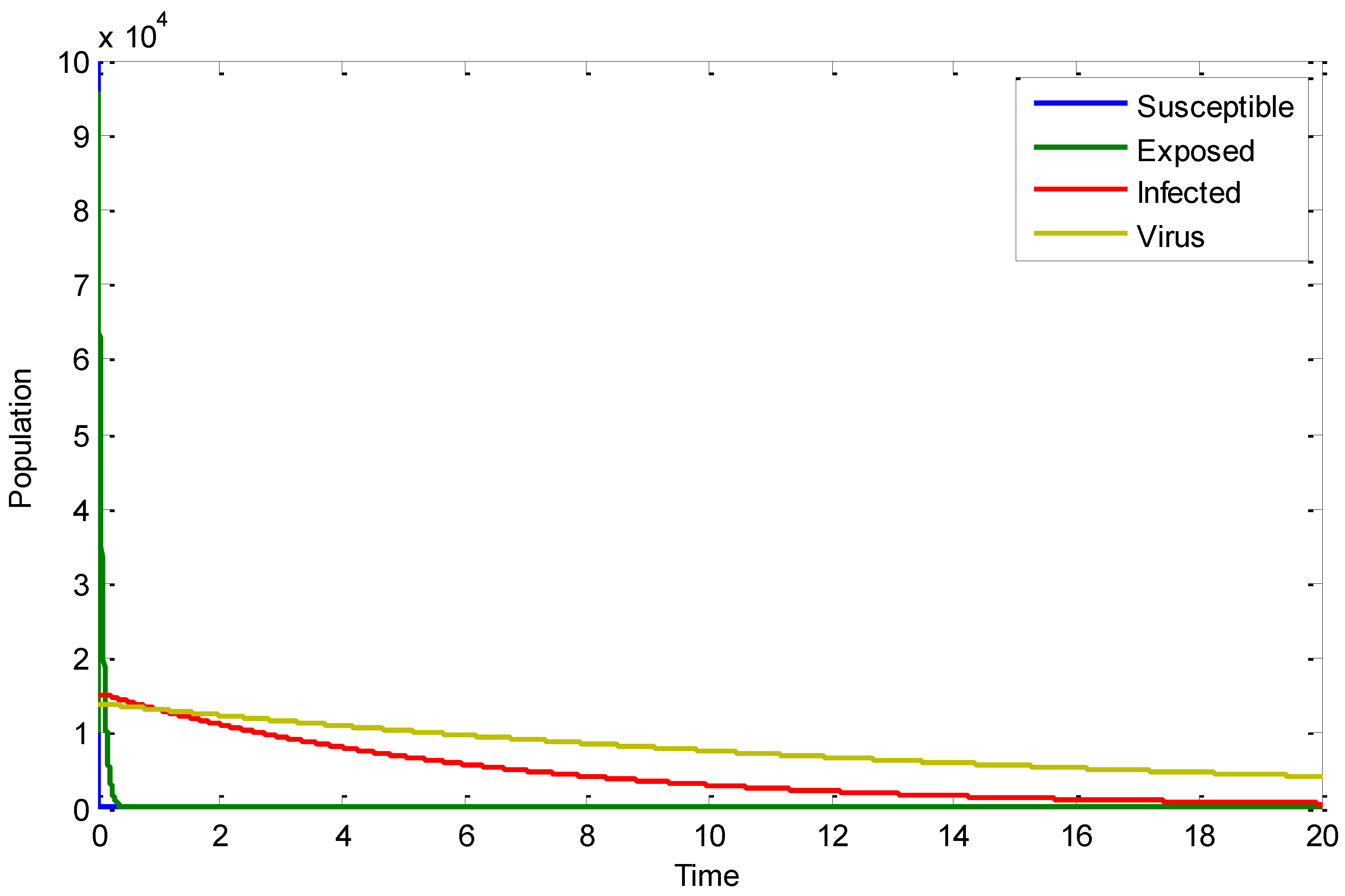
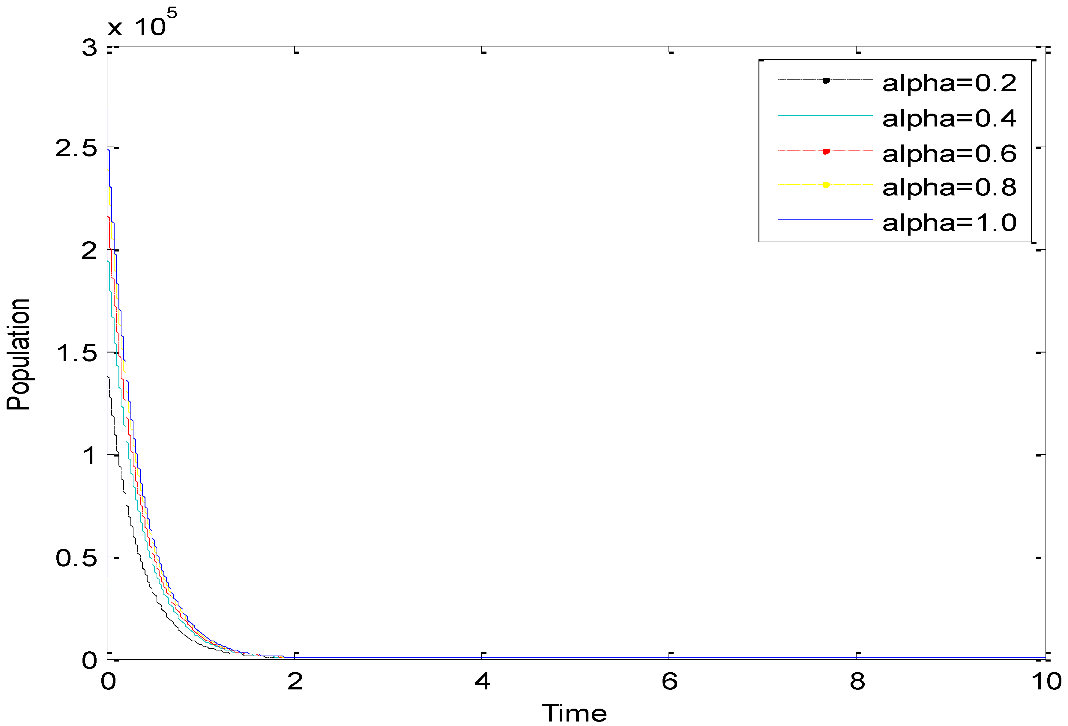
Figure 1 depicts the dynamics of the model. It can clearly be seen that, without shedding effect control, the susceptible populations all go to extinction, whereas infected exposed populations and viral populations proliferate. This clearly shows the need for the application of shedding effect control measures to control the pandemic.

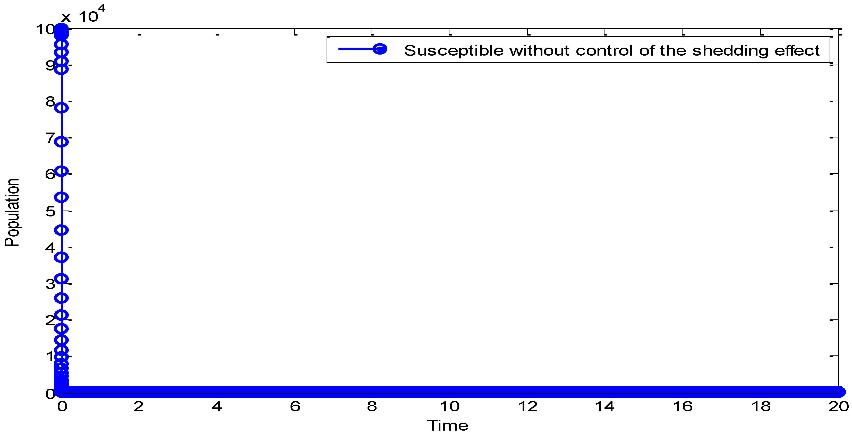
Figure 2 shows the extinction of the variation susceptible population. This means if no control of the shedding effect is observed, subsequently all people in the population will become infected.

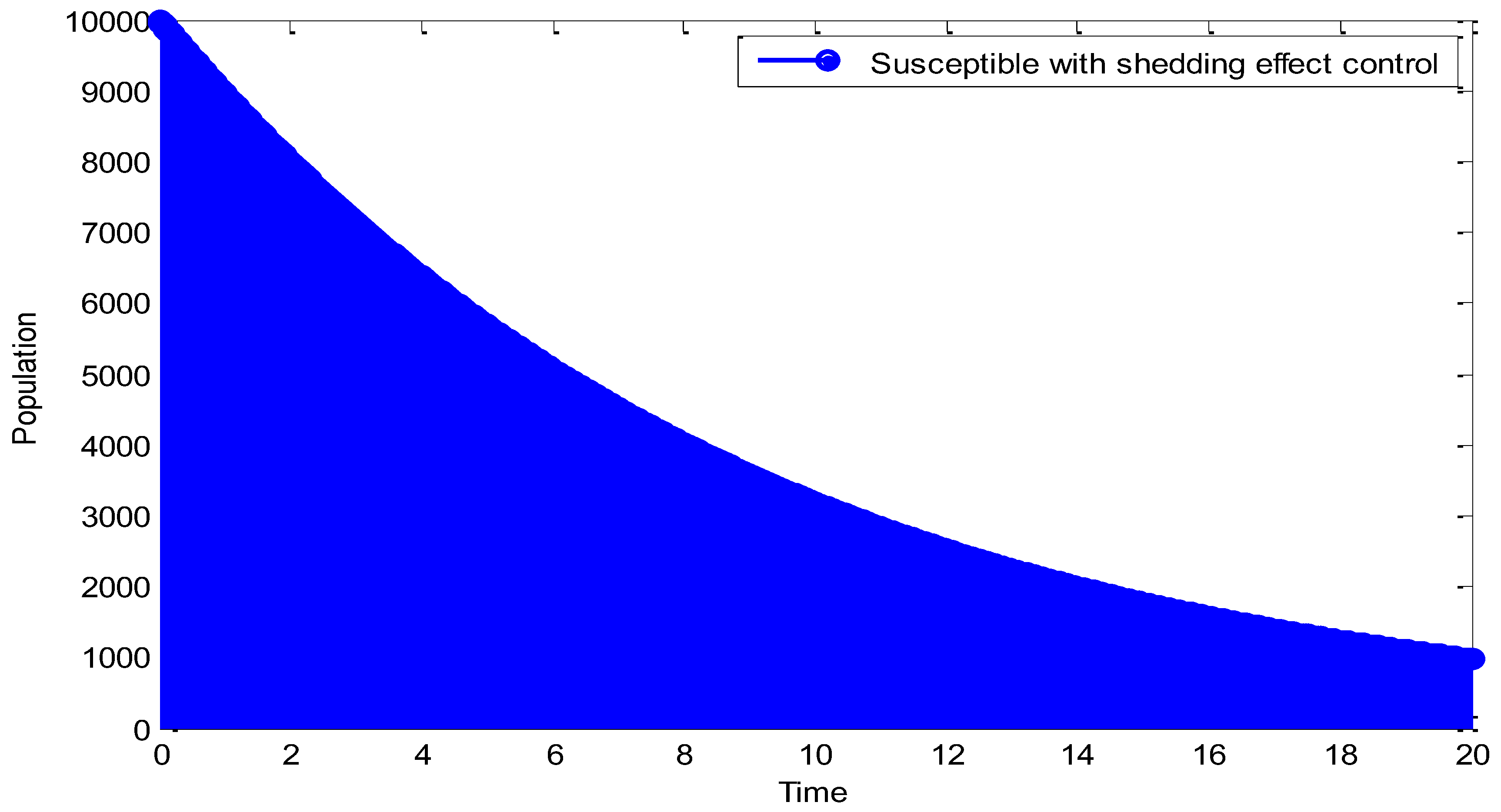
From Figure 3, it can be observed that application of shedding effect control increases the susceptible population. It is clear that there may be a decrease in the population which can be attributed to direct infection of the disease, but the control prevents the population from extinction.

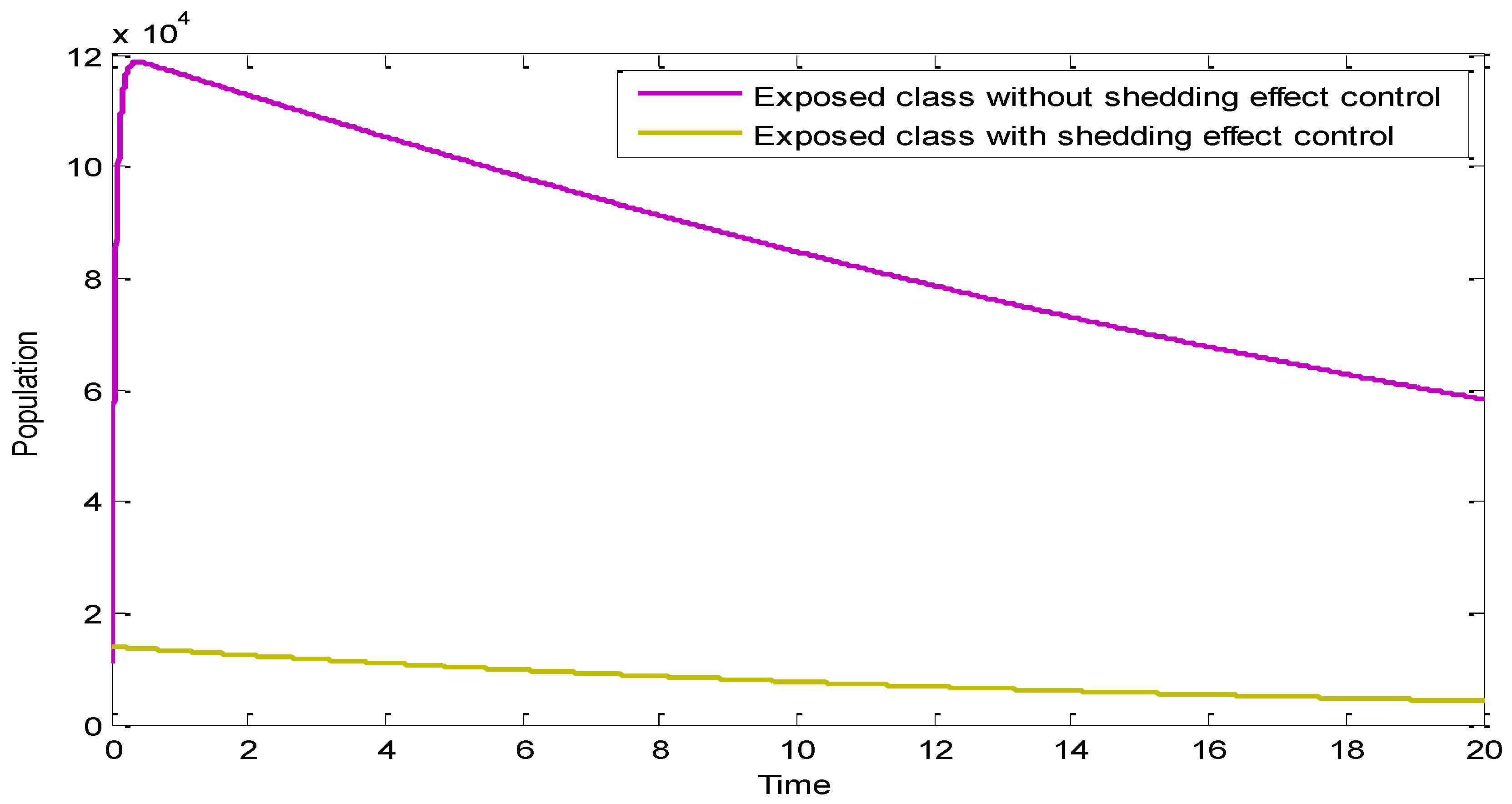
Figure 4 compares the exposed population with and without shedding effect control. It can clearly be seen that application of the control measure has a positive effect on the exposed class as it minimizes it. The proliferation of the disease can be attributed to the direct infection.

Figure 5 compares the infected population with and without shedding effect control. It can clearly be seen that application of the control measure has a positive effect on the infected class as it minimizes it. The proliferation of the disease can be attributed to the direct infection.

Figure 6 shows the influence of the variation in the fractional-order α on the biological behavior of the infected population. It is clear from this Figure that the population has a decreasing effect when α is increased from $0.2 \mathrm{to} 1$. Hence, the memory effect can be seen clearly.

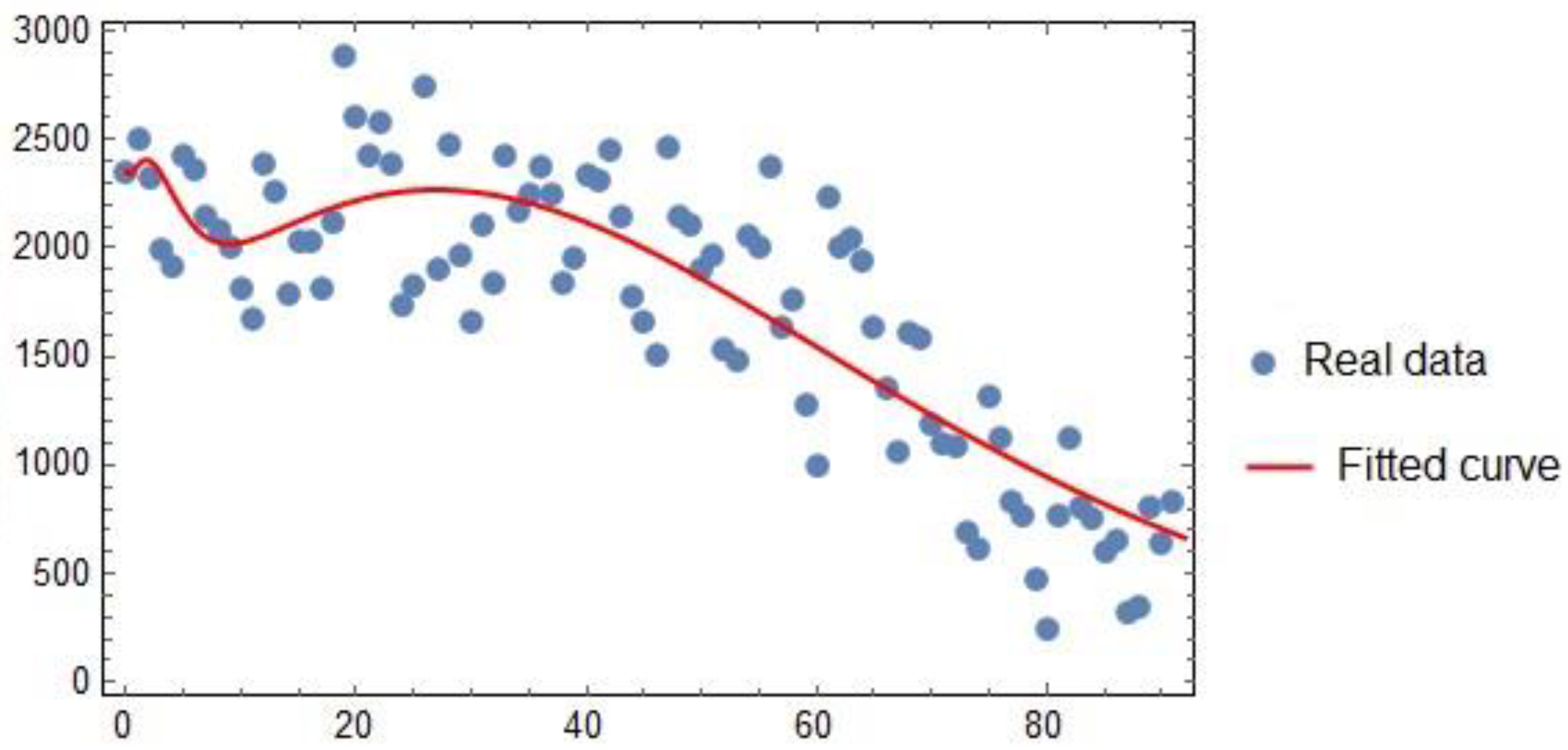
Daily infected cases for Nigeria are used to fit the model. The data are collected from daily new infected cases for Nigeria from 30 January 2020 to 10 April 2020, which is available at the WHO website [34]. Some parameter values were estimated to give the best fit for the model. We fit the curve for daily confirmed cases in Figure 7.

To disclose the plenary scenario of the error analysis, a tabular exposure of the statistical ingredients of error analysis, including minimum value, maximum value, average, and standard deviation (SD) of the relative errors (RE), is provided in

Table 2. Error Analysis of the data prediction for the Infected population.

Minimum Value of RE (%)	Maximum Value of RE (%)	Average RE (%)	SD of RE (%)
0.064410718	5.380764019	1.623503267	1.386483902

.

From the table the error indicated that the result demonstrated better validation of the model in comparison with real data.

7. Summary and Conclusions

This work consists of the transmission dynamics of COVID-19 represented using a fractional order SIR model in the Caputo sense. The model integrates the indirect mode of transmission of COVID-19 which is caused as a result of shedding effect. The indirect mode of transmission of the virus through shedding is an essential factor that needs to be studied. Equilibrium solutions, basic reproduction ratio (that depends both on direct and indirect mode of transmission), existence and uniqueness of the solution of the model and their stabilities were studied. The paper studied the effect of optimal control policy applied to shedding effect. The control is the observation of standard hygiene practices and chemical disinfectants in public spaces. Numerical simulations were carried out and the significance of the fractional order from the biological point of view was established. By applying shedding effect control, it was clear that while the population of susceptible individuals is increased, the populations of exposed and infected individuals are drastically decreased.

The public must follow the government rules or public health care policies to mitigate the spread of the virus. The limitation of this work lies in the absence of more reliable data. This is because more accurate data is needed to obtain better prediction.

We recommend that the fractal approach be used in future to consider the analysis of the model.

References

- Al-Sheikh, S.; Musali, F.; Alsolami, M. Stability Analysis of an HIV/AIDS Epidemic model with screening. Int. Math. Forum 2011, 6, 3251–3273. [Google Scholar]
- Owolabi, K.M.; Atangana, A. Mathematical analysis and computational experiments for an epidemic system with nonlocal and nonsingular derivative. Chaos Solitons Fractals 2019, 126, 41–49. [Google Scholar] [CrossRef]
- Do, T.S.; Lee, Y.S. Modeling the Spread of Ebola. Osong Public Health Res. Perspect. 2016, 7, 43–48. [Google Scholar] [CrossRef]
- Chowell, D.; Chavez, C.C.; Krishna, S.X.; Qiu, K.; Anderson, S. Modelling the effect of early detection of Ebola. Lancet. Infect. Dis. 2015, 15, 148–149. [Google Scholar] [CrossRef]
- Liu, Z.; Magal, P.; Seydi, O.; Webb, G. Predicting the cumulative number of cases for the COVID-19 epidemic in China from early data. Math. Biosci. Eng. 2020, 17, 3040–3051. [Google Scholar] [CrossRef] [PubMed]
- Chen, T.M.; Rui, J.; Wang, Q.P.; Zhao, Z.Y.; Cui, J.A.; Yin, L. A mathematical model for simulating the phase—Based transmissibility of a novel coronavirus. Infect. Dis. Poverty 2020, 9, 24. [Google Scholar] [CrossRef]
- Khan, M.A.; Atangana, A. Modeling the dynamics of novel coronavirus (2019-nCov) with fractional derivative. Alex. Eng. J. 2020, 59, 2379–2389. [Google Scholar] [CrossRef]
- Ivorra, B.; Ferrandez, M.R.; Vela-Perez, M.; Ramos, A.M. Mathematical modeling of the spread of the coronavirus disease 2019, (COVID-19) considering its particular characteristics: The case of China. MOMAT 2020, 88, 105303. [Google Scholar]
- Zamir, M.; Nadeem, F.; Abdeljawad, T.; Hammouch, Z. Threshold condition and non pharmaceutical interventions’s control strategies for elimination of COVID-19. Res. Phys. 2020, 20, 103698. [Google Scholar] [CrossRef]
- Report of the WHO-China Joint Mission on Coronavirus Disease 2019 (COVID-19). Available online: https://www.who.int/china/news/detail/09-01-2020 (accessed on 10 November 2022).
- Becerra, V.M. Optimal control. Scholarpedia 2008, 3, 5354. [Google Scholar] [CrossRef]
- Jajarmi, A.; Ghanbari, B.; Baleanu, D. A new efficient numerical method for the fractional modeling and optimal control of diabetes and tuberculosis co-existence. CHAOS 2019, 29, 093111. [Google Scholar] [CrossRef] [PubMed]
- Baleanu, D.; Jajarmi, A.; Sajjadi, S.S. A new fractional model and optimal control of a tumor-immune surveillance with non-singular derivative operator. CHAOS 2019, 29, 083127. [Google Scholar] [CrossRef] [PubMed]
- Sweilam, N.H.; Al-Mekhlafi, S.M.; Baleanu, D. Optimal control for a fractional tuberculosis infection model including the impact of diabetes and resistant strains. J. Adv. Res. 2019, 17, 125–137. [Google Scholar] [CrossRef] [PubMed]
- Akman, Y.T.; Arshad, S.; Baleanu, D. New observations on optimal cancer treatments for a fractional tumor growth model with and without singular kernel. Chaos Solitons Fractals 2018, 117, 226–239. [Google Scholar] [CrossRef]
- Akman, Y.T.; Arshad, S.; Baleanu, D. Optimal chemotherapy and immunotherapy schedules for a cancer obesity model with caputo time fractional derivative. Math. Methods Appl. Sci. 2018, 18, 9390–9407. [Google Scholar] [CrossRef]
- Baleanu, D.; Joseph, C.; Mophou, G. Low-regret control for a fractional wave equation with incomplete data. Adv. Differ. Equ. 2016, 2016, 240. [Google Scholar] [CrossRef]
- Baba, I.A.; Abdulkadir, R.A.; Esmaili, P. Analysis of tuberculosis model with saturated incidence rate and optimal control. Phys. A Stat. Mech. Its Appl. 2019, 540, 123237. [Google Scholar] [CrossRef]
- Martnez, J.E.E.; Aguilar, J.F.G.; Ramn, C.C.; Melndez, A.A.; Longoria, P.P. Synchronized bioluminescence behavior of a set of fireflies involving fractional operators of LiouvilleCaputo type. Int. J. Biomath. 2018, 11, 1850041. [Google Scholar] [CrossRef]
- Martnez, J.E.E.; Aguilar, J.F.G.; Ramn, C.C.; Melndez, A.A.; Longoria, P.P. A mathematical model of circadian rhythms synchronization using fractional differential equations system of coupled van der Pol oscillators. Int. J. Biomath. 2018, 11, 1850014. [Google Scholar] [CrossRef]
- Ullah, S.; Khan, M.A.; Farooq, M. A fractional model for the dynamics of TB virus. Chaos Solitons Fractals 2018, 116, 63–71. [Google Scholar] [CrossRef]
- Aguilar, J.F.G. Fundamental solutions to electrical circuits of non-integer order via fractional derivatives with and without singular kernels. Eur. Phys. J. Plus 2018, 133, 197. [Google Scholar] [CrossRef]
- Ahmad, S.; Ullah, A.; Al-Mdallal, Q.M.; Khan, H.; Shah, K.; Khan, A. Fractional order mathematical modeling of COVID-19 transmission. Chaos Solitons Fractals 2020, 139, 110256. [Google Scholar] [CrossRef] [PubMed]
- Higazy, M. Novel fractional order SIDARTHE mathematical model of COVID-19 pandemic. Chaos Solitons Fractals 2020, 138, 110007. [Google Scholar] [CrossRef] [PubMed]
- Gao, G.H.; Sun, Z.Z.; Zhang, H.W. A new fractional numerical differentiation formula to approximate the Caputo fractional derivative and its applications. J. Comput. Phys. 2014, 259, 33–50. [Google Scholar] [CrossRef]
- Rabei, E.M.; Almayteh, I.; Muslih, S.I.; Baleanu, D. Hamilton–Jacobi formulation of systems within Caputo’s fractional derivative. Phys. Scr. 2007, 77, 015101. [Google Scholar] [CrossRef]
- Bonyah, E.; Atangana, A.; Khan, M.A. Modeling the spread of computer virus via Caputo fractional derivative and the beta-derivative. Asia Pac. J. Comput. Eng. 2017, 4, 1. [Google Scholar] [CrossRef]
- Abdeljawad, T.; Baleanu, D. On fractional derivatives with exponential kernel and their discrete versions. J. Rep. Math. Phy. 2017, 80, 11–27. [Google Scholar] [CrossRef]
- Atangana, A.; Gómez-Aguilar, J.F. Decolonisation of fractional calculus rules: Breaking commutativity and associativity to capture more natural phenomena. Eur. Phys. J. Plus 2018, 133, 166. [Google Scholar] [CrossRef]
- Singh, A.; Deolia, P. COVID-19 outbreak: A predictive mathematical study incorporating shedding effect. J. Appl. Math. Comput. 2022, 69, 1239–1268. [Google Scholar] [CrossRef]
- Caputo, M.; Fabrizio, M. A new definition of fractional derivative without singular kernel. Prog. Fract. Differ. Appl. 2015, 1, 73–85. [Google Scholar]
- De Oliveira, E.C.; Tenreiro Machado, J.A. A review of definitions for fractional derivatives and integral. Math. Probl. Eng. 2014, 2014, 238459. [Google Scholar] [CrossRef]
- Odibat, Z.; Baleanu, D. Numerical simulation of initial value problems with generalized Caputo-type fractional derivatives. Appl. Numer. Math. 2020, 156, 94–110. [Google Scholar] [CrossRef]
- World Health Organization (WHO) Situation Report. (30 January 2020–30 April 2020). Available online: http://www.who.int (accessed on 1 December 2022).