Article

Optimal Consumption, Investment, and Housing Choice: A Dynamic Programming Approach

1
Department of Mathematics, Pusan National University, 2 Busandaehak-ro 63beon-gil, Geumjeong-gu, Busan 46241, Korea
2
Division of Business Administration, Pukyong National University, 45 Yongso-ro, Nam-gu, Busan 48513, Korea
*
Author to whom correspondence should be addressed.
Axioms 2022, 11(3), 127; https://doi.org/10.3390/axioms11030127
Submission received: 29 January 2022 / Revised: 9 March 2022 / Accepted: 10 March 2022 / Published: 11 March 2022
(This article belongs to the Special Issue Mathematical Analysis for Financial Modelling)

Abstract

:
We investigate a portfolio selection problem involving an agent’s realistic housing service choice, where the agent not only has to choose the size of house to live in, but also has to select between renting and purchasing a house. Adopting a dynamic programming approach, we derive a closed-form solution to obtain the optimal policies for the consumption, investment, housing service, and purchasing time for a house. We also present various numerical demonstrations showing the impacts of parameters in the financial and housing markets and the agent’s preference, which visually show the economic implications of our model. Our model makes a significant contribution because it is a pioneering model for the optimal time to purchase a house, which has not been investigated in depth in existing mathematical portfolio optimization models.

1. Introduction

A house is one of the most important assets in a person’s life. A person receives the utility of living in the house, while it simultaneously plays the role of an investment asset as the value of the house fluctuates. Thus, many people have housing-related concerns such as which house to live in, whether to rent or buy a house, and when to buy a house.
However, there are relatively few mathematical and theoretical models for such housing concerns. Although there have been many mathematical financial studies dealing with the topic of individual optimal choice, including those dealing with optimal consumption, optimal investment, or optimal retirement, it is not easy to find a study dealing with optimal housing choice. As previously mentioned, housing can also be viewed as a risky investment. Yet, most studies on risky assets consider stocks. However, the stocks themselves have absolutely no practical usefulness to the agent in terms of utility, no matter how many stocks they own. Conversely, a house delivers a very direct utility to the agent, and everyone must have at least one house to live in, whether it is rented or purchased. Therefore, their choice of a house must include a consideration of the utility to the agent, which is a significant difference from stocks.
In this context, we extend the general consumption and investment problem of an agent to propose an optimization problem that includes the agent’s housing service choice. The agent in this study has a Cobb–Douglass type utility function of consumption and housing, which is used to determine the size of the house in which to live, along with the consumption and investment. To simplify the model, we consider one type of house, just as a single consumption asset is considered in most optimal consumption choice models. Therefore, the optimal housing choice for the agent is the selection of the size of the house.
In addition, we model the agent’s optimal choice between renting and purchasing a house. This is an optimal stopping problem, in which the agent rents at a low wealth level because the agent cannot afford the cost of buying a house, but when the agent reaches a certain level of wealth, the agent pays for a house and lives there. We model this optimal stopping problem with respect to housing and investigate the wealth level at which the agent chooses to switch from renting to owning. This can be seen as similar to financial mathematical models that consider the optimal retirement time. For simplicity of the model, we assume that the agent trades houses continuously during the rental period, but no longer switches between houses after purchasing a house. This is because many people tend to move relatively frequently before they actually own a house (i.e., while renting), but once they purchase a house, the frequency of moving significantly decreases because of the high transaction costs. In other words, there is a large difference between choosing a house to rent and a house to purchase and live in. People are more conservative when choosing a house they will buy and live in, and tend to choose a house that they are willing to live in for a long time. This is in line with the argument of [1] that durable assets such as houses are very difficult to adjust because of their high transaction costs and that of [2] that the liquidation cost reduces the trading of housing assets. Moving out of a purchased house probably has a much higher transaction cost than moving out of a rented one.
We apply a dynamic programming approach developed by [3] to find the closed-form solution to the model and provide a detailed proof. Moreover, several numerical demonstrations are presented to derive the economic implications of the solution. The results allow us to examine how various economic variables affect the agent’s optimal choice, including consumption, investment, and housing. In particular, because the main interest of this study is the housing choice, the results related to this are briefly summarized as follows. First, we show that as the expected rate of return on risky assets or risk-free assets in the financial market decreases, the optimal timing of purchasing a house is delayed. This is because high-liquid financial assets are needed for consumption even after purchasing a house, which is a large expenditure. Thus, when high returns are expected in the financial market, the agent purchases a house at an early stage. In addition, as the housing price rises, because the burden of rental cost rises, the optimal time to purchase a house is earlier. As the growth rate of housing price increases, ceteris paribus, the purchase of a house is delayed in order to enjoy the undervalued housing services for a longer period of time. We also offer a variety of comparative statics related to consumption and investment in the numerical demonstrations.
The rest of this paper is structured as follows. Section 2 provides a brief survey of studies related to ours. We present the theoretical model in Section 3 and derive the analytic solution in Section 4. In Section 5, we show numerical demonstrations of the solution and discuss their implications. This study is concluded in Section 6.

2. Related Literature

After the pioneering research of [4,5], an enormous number of rigorous mathematical models in a continuous time of consumption and investment optimization problems have been studied and extended to various applications. These include studies on an agent’s labor-leisure choice and voluntary retirement [6,7,8,9,10,11,12], on optimization given certain borrowing constraints [8,13,14,15,16,17], and on an agent’s subsistence consumption constraint or consumption habit [9,18,19,20,21,22].
Among these, the studies most closely related to ours are those modeling an agent’s optimal stopping time. Most of these model the disutility from labor [6,9,10] or the increase in utility from leisure [7,11,12], and analyze the optimal voluntary retirement time of an agent. References [6,7] are pioneering studies on modeling the disutility and leisure of agents, respectively. Reference [9] studies the optimal portfolio selection of an agent with disutility and subsistence consumption using the martingale method, and [10] investigate a problem that is almost similar to [9] using the dynamic programming approach. In addition, Ref. [11] study the optimal leisure choice of an agent with the constant elasticity of substitution (CES) utility, and [12] does this with the Cobb–Douglas utility. However, no studies considering housing choice or utility from housing can be found in these studies to model optimal stopping problems.
We solve our problem using the dynamic programming approach, which is developed by [3], just as in many previous consumption and investment optimization studies. Among the studies mentioned above, Refs. [6,10,12,19,21] use this approach. In particular, Ref. [19] investigate the role of index bonds in an optimal portfolio selection problem given a subsistence consumption constraint, and [21] study an optimal consumption and investment problem using a quadratic utility function.
As seen so far, it is difficult to find models dealing with the utility from housing or optimal housing choice problems, especially in a continuous time. Recently, Ref. [23] study a lessor’s choice of renting a house given a borrowing constraint, but they do not consider housing choices or the utility from housing.
Instead, among the discrete-time models, Refs. [2,24,25,26,27] can be cited as studies related to ours. Among these studies, Ref. [24] could be considered to be the closest to our study. They investigate a portfolio selection problem that includes rental and purchase options. However, they model a very complex discrete-time problem that includes short-sale constraints and stochastic labor income, and only present the numerical results without deriving an analytic solution at all. In addition, unlike our model, they assume that even an agent who owns a single house frequently trades the house as if the house were an investment asset, which is a bit far from reality. Reference [2] studies optimal stock and housing investment, and [25] considers the housing and investment demands of retirees, but these studies are also different from ours because they do not consider the decision between renting and owning a house. On the other hand, Ref. [26] investigate the optimal investments of agents holding risky housing assets, using a mean-variance efficiency framework, and [27] consider the impact of housing on an agent’s investment, distinguishing between the effects of home equity and mortgage debt.
Recently, many studies have been proposed that reflect the phenomenon in which the volatility of the asset price process changes over time in the model by introducing a jump-diffusion process [28,29] or a stochastic volatility of asset price process [30,31,32]. These models aim to more precisely estimate the movement of asset prices, and are being actively applied not only to the pricing of financial products, but also to the optimal investment problem of individuals who invest in these products. There are also a bunch of literature in a slightly different direction from these studies that considered fractional Brownian motion [33,34]. Those studies considering a jump-diffusion process or a stochastic volatility mentioned above usually solve extended Merton problem following a standard Brownian motion rather than a fractional Brownian motion.
This study does not reflect a stochastic volatility or a fractional Brownian motion of asset price processes, but for parsimony, considers a constant volatility to focus on the optimal stopping time to purchase a house rather than the risky investment behavior of individuals. If a stochastic volatility or a fractional Brownian motion is considered, a more realistic asset price process can be modeled, but the constant volatility is also sufficient to derive fundamental economic implications for the optimal stopping time to purchase a house.
In summary, our study is very original because there has been no other study dealing with an agent’s utility from housing and optimal housing choice in a continuous time, and it is also difficult to find similar studies among discrete time models.

3. Model

In this study, it is assumed that the agent participates in a continuous-time financial market in which a risky asset and risk-free asset are traded. The market is also assumed to be frictionless, that is, there is no tax, no transaction cost, and no limitation on financial market participation. The risk-free asset, denoted S t 0 , has a positive fixed interest rate, r, and can be defined as follows:
d S t 0 S t 0 = r d t .
The risky asset, S t , follows a geometric Brownian motion with a constant drift, μ , and a constant volatility, σ , such that
d S t S t = μ d t + σ d B t ,
where B t is a standard Brownian motion under the standard probability measure ( Ω , F t , P ) .
Let c t and π t denote the consumption rate and portfolio process, respectively. The consumption rate is assumed to be non-negative and progressively measurable with respect to F t for all t 0 , with the condition 0 c s d s < almost surely (a.s.). The portfolio process is the dollar amount investment in the risky asset and is also assumed to be a F t -measurable process with 0 π s 2 d s < , a.s.
In addition, we consider the housing process, h t , which is also assumed to be F t -measurable with 0 h s d s < . It is assumed that the agent needs a house to live in, whether the agent rents or purchases the house, and h t represents the size of the house, that is, the agent chooses the size of the house endogenously. If the agent rents a house, they have to pay the rental cost, which is proportional to the size of the house, or, if the agent purchases, they have to pay the price of the house in a lump sum at the time of the purchase, which is also proportional to the size of the house.
In addition, it is also assumed that the agent receives a constant income from labor, I. In sum, the wealth process of the agent is governed by
d X t = r X t + ( μ r ) π t c t + I 1 { 0 t < τ p } · R t h t d t + σ π t d B t , X 0 = x ,
where X t is the financial wealth level of the agent at time t, τ p is the endogenous time of purchasing a house, 1 { t τ p } is an indicator function that has the value of 1 before the agent’s purchase and 0 after, and R t is the housing rental cost rate at time t for the housing unit. Here, R t is computed as the product of the unit price of the house, P t , and the rental cost rate, δ , that is, R t = δ P t , where the unit price follows
d P t P t = μ h d t + σ h d B t , P 0 = p .
In addition, to simplify the model, it is assumed that the agent chooses the optimal housing size, h t , continuously before the time of purchase, τ p , but after τ p , the agent no longer trades the house. Most people move relatively frequently when renting a house, but once they purchase a house, they usually stop moving frequently because of the high transaction costs [1,2]. Let h ¯ denote the size of the house purchased by the agent.
The optimal consumption, investment, and housing problem of the agent can be described as follows.
Problem 1.
Given initial wealth x and constant labor income I, the agent wishes to maximize the expected utility from life-time consumption and housing by choosing consumption rate { c t } , portfolio process { π t } , housing rate (size) { h t } , purchasing time τ p , and terminal housing rate h ¯ :
V ( x , p ) = max c t , π t , h t , τ p , h ¯ E 0 e β t c t α h t 1 α 1 γ 1 γ 1 0 t < τ p + κ c t α h ¯ 1 α 1 γ 1 γ 1 τ p t d t max c t , π t , h t , τ p , h ¯ E 0 τ p e β t c t α h t 1 α 1 γ 1 γ d t + e β τ p V ¯ ( X τ p , h ¯ )
subject to the budget constraint (2), where β is the subjective discount rate, α is the coefficient of constant elasticity of substitution between consumption and housing, γ is the coefficient of relative risk aversion, and κ is the constant of preferences for owing a house to live in. V ¯ ( x , h ¯ ) is the value function after purchasing, that is, living in the agent’s own house.

4. Analytic Solutions

To solve Problem 1, we first derive V ¯ ( x , h ¯ ) in the following subsection, and then obtain V ( x , p ) , using V ¯ ( x , h ¯ ) derived.

4.1. Value Function after Time of Purchase

After purchasing a house, the agent pays no rent, and thus the agent’s wealth dynamics is as follows:
d X t = r X t + ( μ r ) π t c t + I d t + σ π t d B t , X 0 = x .
Based on the definition of V ¯ ( x , h ¯ ) in Problem 1, we can write the following problem to find V ¯ ( x , h ) .
Problem 2
(Problem after Purchasing). Given initial wealth x and housing size h ¯ , the agent wishes to maximize the expected utility from life-time consumption by choosing consumption rate { c t } and portfolio process { π t } :
V ¯ ( x , h ¯ ) = max c t , π t E 0 e β t κ c t α h ¯ 1 α 1 γ 1 γ d t
subject to the budget constraint (5).
Let us define the function and inverse function of the consumption rate with respect to the wealth level as follows.
Definition 1.
Let consumption rate c = C ( x ) , where c is a function of the wealth level. We can define the inverse function of C ( x ) to be C 1 ( · ) = X ( · ) , namely, X ( c ) = X ( C ( x ) ) = x .
With the function in Definition 1, we can obtain the closed-form solution of V ¯ ( x , h ¯ ) in the following theorem.
Theorem 1.
The closed-form solutions of the value function V ¯ ( x , h ¯ ) , the optimal consumption rate and portfolio process in Problem 2, are given by the following:
V ¯ ( x , h ¯ ) = h ¯ ( 1 α ) ( 1 γ ) Υ ( c * ) α ( 1 γ ) ,
c t * = M X t + I r , π t * = θ σ 1 α ( 1 γ ) 1 X t + I r ,
where
Υ = 1 β 1 α ( 1 γ ) 1 γ + α M r θ 2 2 ( α ( 1 γ ) 1 ) κ 1 γ ,
M = r + r β α ( 1 γ ) 1 1 2 θ 2 α ( 1 γ ) ( α ( 1 γ ) 1 ) 2 .
When α = 1 , M in (10) is rewritten as follows:
r + β r γ + ( γ 1 ) θ 2 γ 2 ,
which is exactly the same as the equation given by [4]. This is natural in the sense that if α = 1 , the agent gets no utility from the housing service, and the problem becomes a general consumption and portfolio optimization problem without the housing choice.
The brief proof of Theorem 1 is as follows. Adopting the dynamic programming approach, we obtain the following Hamilton–Jacobi–Bellman (HJB) equation:
β V ¯ = max c , π ( r x + ( μ r ) π c + I ) V ¯ ( x ) + 1 2 σ 2 π 2 V ¯ ( x ) + u ( c ) ,
where
u ( c ) = κ c α h ¯ 1 α 1 γ 1 γ .
From first-order conditions with respect to the two decision variables, c and π , we can rewrite (11) as follows:
β V ¯ = ( r x + I ) V ¯ ( x ) 1 2 θ 2 V ¯ ( x ) 2 V ¯ ( x ) + max c u ( c ) c V ¯ ( x ) .
Using the consumption rate function in Definition 1, (12) is rewritten as follows:
β V ¯ ( X ( c ) ) = ( r X ( c ) + I ) α κ 1 γ h ¯ ( 1 α ) ( 1 γ ) c α ( 1 γ ) 1 1 2 θ 2 α κ 1 γ h ¯ ( 1 α ) ( 1 γ ) c α ( 1 γ ) X ( c ) α ( 1 γ ) 1 + 1 α ( 1 γ ) 1 γ κ 1 γ h ¯ ( 1 α ) ( 1 γ ) c α ( 1 γ ) .
Taking the derivative of (13) with respect to c, we obtain the second-order ODE as follows:
0 = 1 2 θ 2 1 α ( 1 γ ) 1 c 2 X ( c ) + r β 1 2 θ 2 α ( 1 γ ) α ( 1 γ ) 1 c X ( c ) + r [ α ( 1 γ ) 1 ] X + I [ α ( 1 γ ) 1 ] [ α ( 1 γ ) 1 ] c .
Solving (14), we obtain value function V ¯ ( x , h ¯ ) and, consequently, the optimal policies in Theorem 1.

4.2. Value Function before Time of Purchase

Before purchasing a house, the agent pays rent. Thus, the agent’s wealth dynamics is as follows:
d X t = r X t + ( μ r ) π t c t + I R t h t d t + σ π t d B t , X 0 = x ,
where R t = δ P t .
To solve Problem 1 analytically, we first introduce the following Lemma.
Lemma 1.
We consider V ( x , p ) = p α ( 1 γ ) V ˜ ( x ˜ ) by the following variable changes:
I ˜ I p , c ˜ c p , π ˜ π p , x ˜ x p .
For later use, we also consider a quadratic equation in the remark below.
Remark 1.
m < 1 and m + > 0 are the real roots of the following quadratic equation:
1 2 θ ˜ 2 m 2 + β ˜ r ˜ + 1 2 θ ˜ 2 m r ˜ = 0 ,
where
β ˜ = β μ h α ( 1 γ ) 1 2 σ h 2 α ( 1 γ ) 1 α ( 1 γ ) , θ ˜ = θ + σ h [ α ( 1 γ ) 1 ] , r ˜ = r μ h + θ σ h .
Thus, we have
m + = β ˜ + r ˜ 1 2 θ ˜ 2 + β ˜ r ˜ + 1 2 θ ˜ 2 2 + 2 θ ˜ 2 r ˜ θ ˜ 2 , m = β ˜ + r ˜ 1 2 θ ˜ 2 β ˜ r ˜ + 1 2 θ ˜ 2 2 + 2 θ ˜ 2 r ˜ θ ˜ 2 .
When 0 t τ p , the following theorem describes the solution to Problem 1.
Theorem 2.
The closed-form solutions of value function V ( x , p ) , the optimal consumption rate, portfolio process, size of the house, and purchasing time in Problem 1, take the following form:
V ( c ˜ , p ) = 1 β ˜ p α ( 1 γ ) B 1 c ˜ γ m γ η 3 ( 1 γ ) α r ˜ 1 2 θ ˜ 2 m + 1 β ˜ p α ( 1 γ ) c ˜ 1 γ η 3 γ + 1 K ( 1 γ ) 1 2 γ θ ˜ 2 + r ˜ , c * c ˜ t * , P t = c ˜ t * P t , π * c ˜ t * , P t = σ h B 1 ( c ˜ t * ) γ m + 1 α K c ˜ t * I ˜ r ˜ P t σ + η 2 c ˜ t * γ B 1 m ( c ˜ t * ) γ m 1 + 1 α K P t σ 2 γ , h * c ˜ t * = 1 α α δ c ˜ t * , h ¯ * = ( 1 α ) ( 1 γ ) Υ c ˜ τ p ̲ α κ 1 γ η , τ p ̲ = inf t 0 : X t ˜ X ˜ τ p ̲ ,
where
K = r ˜ + β ˜ r ˜ γ + γ 1 2 γ 2 θ ˜ 2 ,
and c ˜ t * satisfies the following equation:
X ˜ t * = B 1 ( c ˜ t * ) γ m + 1 α K c ˜ t * I ˜ r ˜ ,
and the threshold, c ˜ τ p ̲ , corresponding to the optimal purchasing time, τ p ̲ , is characterized by
c ˜ τ p ̲ = I ˜ r ˜ I ˜ r η 5 η 4 + 1 α K 1 M η ( 1 α ) ( 1 γ ) Υ α κ 1 γ η 1 ,
and the threshold X ˜ τ p ̲ corresponding to the optimal purchasing time τ p ̲ is determined by
X ˜ τ p ̲ = B 1 c ˜ τ p ̲ γ m + 1 α K c ˜ τ p ̲ I ˜ r ˜ .
Coefficient B 1 is given by
B 1 = η 5 η 4 c ˜ τ p ̲ 1 + γ m ,
where
η 3 = ( 1 α α δ ) ( 1 α ) ( 1 γ ) 1 γ , η 4 = 1 β ˜ η 3 ( 1 γ ) α r ˜ 1 2 θ ˜ 2 m , η 5 = 1 β ˜ η 3 γ + 1 K ( 1 γ ) 1 2 γ θ ˜ 2 + r ˜ ( 1 α ) ( 1 γ ) Υ α κ 1 γ ( 1 α ) ( 1 γ ) Υ η γ 1 ,
η = κ ( 1 γ ) [ ( 1 α ) ( 1 γ ) 1 ] γ η 3 ( 1 γ ) 1 γ ( 1 α ) ( 1 γ ) Υ α ( 1 α ) ( 1 γ ) γ .
Proof. 
The proof of Theorem 2 is carried out using the following three steps. A detailed supplementary proof is provided in Appendix A.
Step 1. In this step, we develop a dynamic programming approach to resolve Problem 1. We apply changes to the variables in Lemma 1 to convert the value function in Problem 1 into the product of the power of the unit price of the house and a one-variable function. That is, we need to convert the following HJB equation into an ODE:
β V = max c , π , h { r x + ( μ r ) π c δ p h + I } V x + 1 2 σ 2 π 2 2 V x 2 + μ h p V p + 1 2 σ h 2 p 2 2 V p 2 + σ σ h π p 2 V x p + u ( c , h ) ] ,
where
u ( c , h ) = c α h 1 α 1 γ 1 γ .
To obtain an ODE from (21), we apply Lemma 1. Then, the HJB equation in (21) can be rewritten as follows:
β ˜ V ˜ = max c ˜ , π ˜ , h η 1 x ˜ + η 2 π ˜ c ˜ δ h + I ˜ V ˜ ( x ˜ ) + 1 2 σ 2 π ˜ 2 2 1 σ σ h π ˜ x ˜ + 1 2 σ h 2 x ˜ 2 V ˜ ( x ˜ ) + u ( c ˜ , h ) ] ,
where
η 1 = r μ h σ h 2 [ α ( 1 γ ) 1 ] ,
η 2 = σ [ θ + σ h ( α ( 1 γ ) 1 ) ] ,
u ( c ˜ , h ) = c ˜ α ( 1 γ ) h ( 1 α ) ( 1 γ ) 1 γ .
Step 2. In the second step, we apply Definition 1 to c ˜ and x ˜ . Similarly, (22) can be switched into a second-order ODE for c ˜ . Then, we can characterize the closed-form solution of x ˜ . Under the assumptions that V ˜ ( x ˜ ) > 0 and V ˜ ( x ˜ ) < 0 , from the first-order conditions with respect to c ˜ , π ˜ , and h, we obtain the following:
h * = 1 α α δ c ˜ * ,
c ˜ * = V ˜ ( x ˜ ) 1 γ η 3 ( 1 γ ) α 1 γ ,
π ˜ * = σ σ h x ˜ V ˜ ( x ˜ ) η 2 V ˜ ( x ˜ ) σ 2 V ˜ ( x ˜ ) ,
where η 3 is found as shown in (19).
Substituting (26) and (28) into (22), we can rewrite (22) as follows:
β ˜ V ˜ = η 1 + σ h η 2 σ x ˜ + I ˜ V ˜ ( x ˜ ) + max c ˜ c ˜ 1 γ η 3 1 α c ˜ V ˜ ( x ˜ ) 1 2 η 2 2 V ˜ ( x ˜ ) 2 σ 2 V ˜ ( x ˜ ) .
Applying Definition 1 to the variables changed in step 1, (29) can be modified as follows:
β ˜ V ˜ X ˜ ( c ˜ ) = η 1 + σ h η 2 σ X ˜ ( c ˜ ) + I ˜ η 3 ( 1 γ ) α c ˜ γ + η 3 γ c ˜ 1 γ + 1 2 η 2 2 η 3 ( 1 γ ) α X ˜ ( c ˜ ) c ˜ 1 γ σ 2 γ .
Now let us take the derivative of (30) with respect to c ˜ . Then, (30) can be converted into a second-order ODE as follows:
0 = 1 2 γ θ ˜ 2 c ˜ 2 X ˜ ( c ˜ ) + r ˜ β ˜ + 1 γ 2 γ θ ˜ 2 c ˜ X ˜ ( c ˜ ) r ˜ γ X ˜ + γ α c ˜ γ I ˜ .
Applying Remark 1, we obtain the closed-form solution of the second-order ODE (31) as follows:
X ˜ ( c ˜ ) = B 1 c ˜ γ m + 1 α K c ˜ I ˜ r ˜ ,
where the unknown coefficient, B 1 , will be determined later.
Step 3. In the final step, we derive the analytical solution of V ˜ and use boundary conditions to determine the threshold consumption rate at the purchasing time. Notice that the agent has to pay P τ p h ¯ to buy the house at the stopping time of purchasing, τ p . In other words, X τ p in (4) must be X τ p ̲ P τ p h ¯ , where τ p ̲ is the time infinitesimally before τ p . Substituting (32) into (30), the closed-form solution of V ˜ can be characterized as follows:
V ˜ ( x ˜ ) = 1 β ˜ B 1 c ˜ γ m γ η 3 ( 1 γ ) α r ˜ 1 2 θ ˜ 2 m + 1 β ˜ c ˜ 1 γ η 3 γ + 1 K ( 1 γ ) 1 2 γ θ ˜ 2 + r ˜ .
At purchasing time τ p , we have
V ( X τ p ̲ ) = max h ¯ V ¯ ( X τ p , h ¯ ) .
Let us first find the relationship between h ¯ and c τ p , that is, the optimal housing after τ p and the consumption rate at τ p . Taking the first-order condition of (34) with respect to h ¯ , we obtain the optimal size of the house to purchase as follows:
h ¯ * = ( 1 α ) ( 1 γ ) Υ c τ p α κ 1 γ P τ p .
Then, let c τ p ̲ = η c τ p , with η ( 1 , ) , and we have c ˜ τ p ̲ = c τ p ̲ P τ p = η c τ p P τ p = η c ˜ τ p .
According to the smooth-pasting condition, V ( X τ p ̲ ) = V ¯ ( X τ p ) , from (27), (35), and the first-order condition with respect to c of (11), we can determine η as in (20). In addition, according to the value-matching condition, V ( X τ p ̲ ) = V ¯ ( X τ p ) , from (7), (33), and (35), we can characterize B 1 as in (18). Finally, we apply the variable changes to X τ p ̲ = X τ p + P τ p h ¯ , that is, X ˜ τ p ̲ = X ˜ τ p + h ¯ . Then, from (8), (32), and (35), we obtain c ˜ τ p ̲ as in (17). □
For a benchmark problem, we consider the following.
Problem 3.
Given initial wealth x and constant labor income I, the agent wishes to maximize the expected utility from life-time consumption and housing by choosing consumption rate { c t } , portfolio process { π t } , and housing rate (size) { h t } :
V b ( x , p ) = max c t , π t , h t E 0 e β t c t α h t 1 α 1 γ 1 γ d t
subject to the following budget constraint
d X t = r X t + ( μ r ) π t c t + I R t h t d t + σ π t d B t , X 0 = x .
The agent in the benchmark problem in Problem 3 does not buy any house over his/her lifetime. Thus, the agent always rents a house and pays the rental cost. This problem is just a typical portfolio optimization problem, and we provide the solution in Appendix A. However, the solution is numerically presented with the solution to our model, for comparative analysis in the following section.

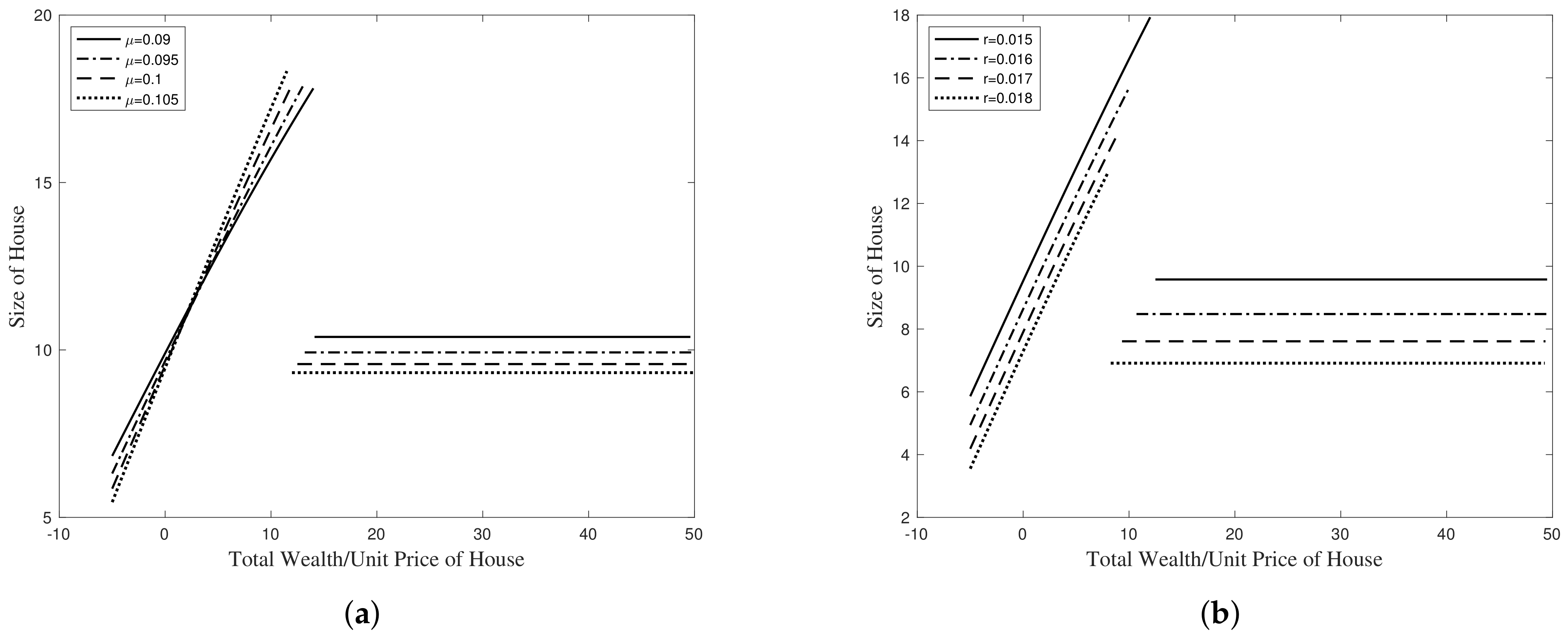
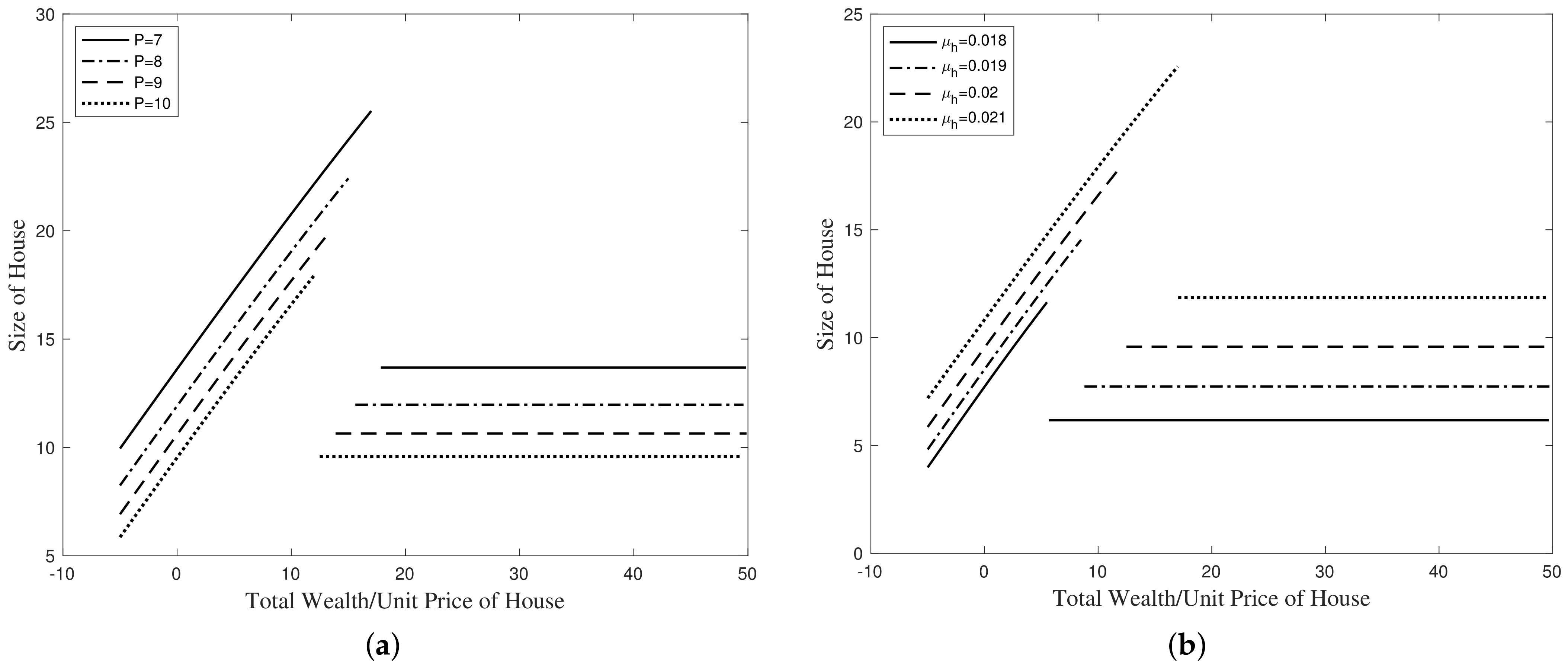
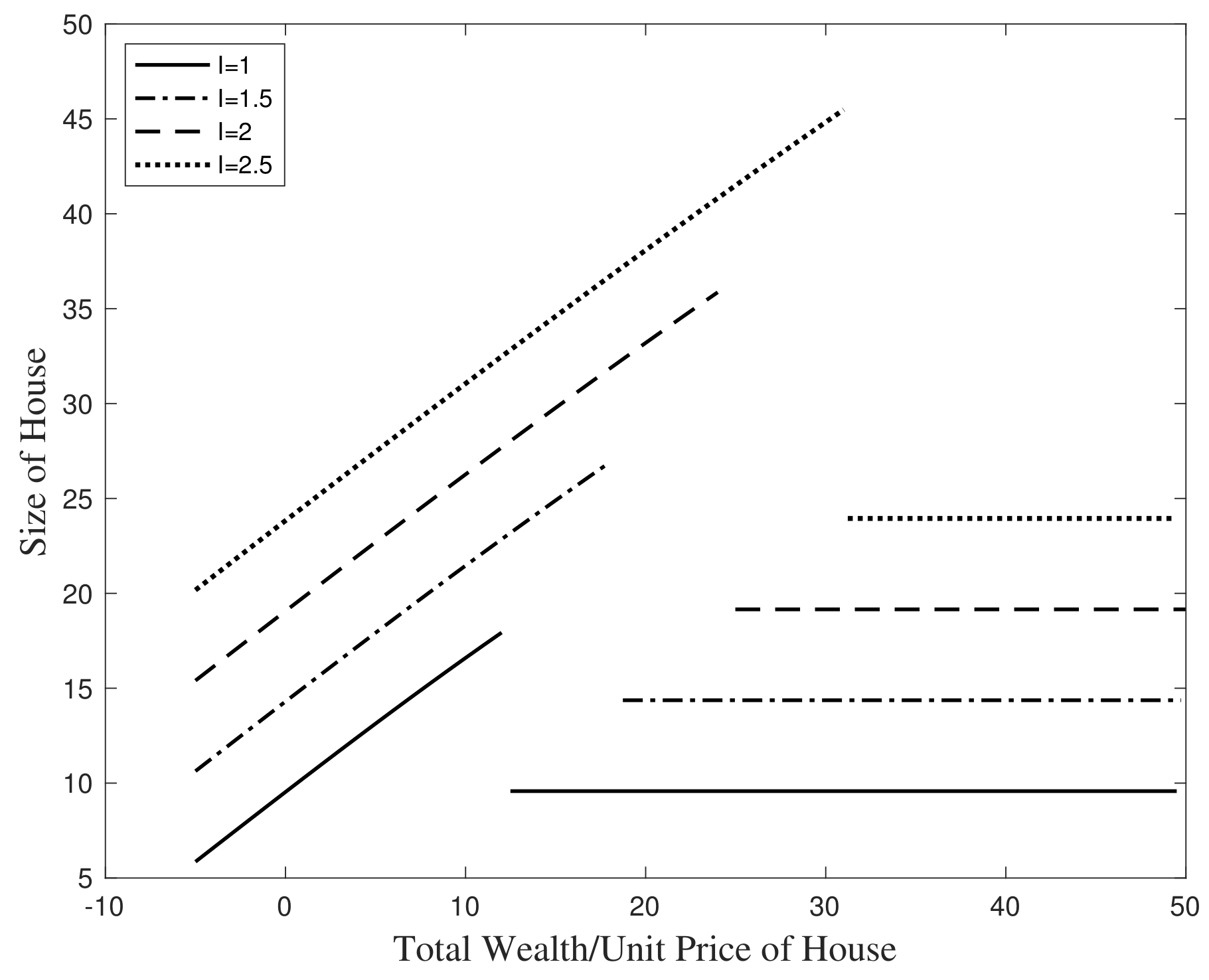
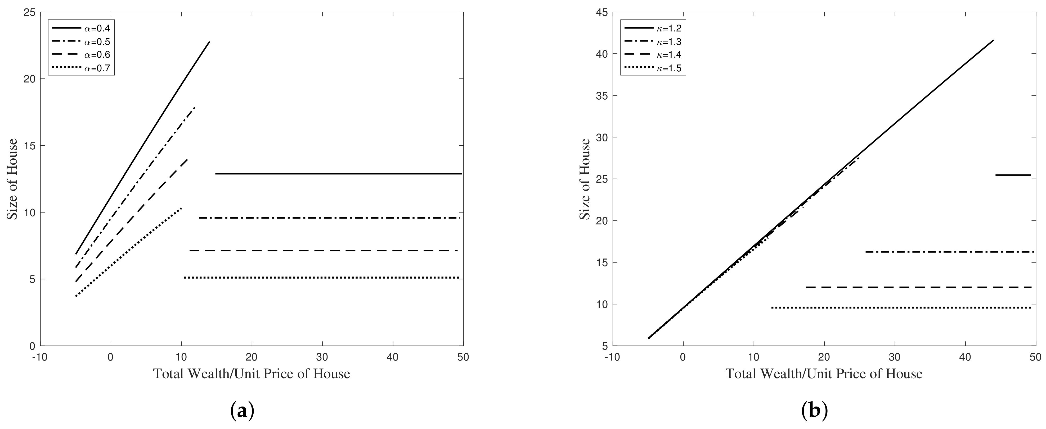
5. Numerical Demonstrations and Implications

Although we derived a closed-form solution in the previous section, it is difficult to find the economic implications because the solution is very complex. Instead, we present numerical and graphical demonstrations and try to find the economic implications by examining the changes in the optimal policies of the agent in Theorem 2, according to the changes in various parameters in this section.
For the graphical demonstrations, we choose the following set of parameter values for the market and the agent’s preference, which will be the baseline values for the comparative statics:
β = 0.01 , γ = 3 , r = 0.015 , α = 0.5 , I = 1 , P = 10 , κ = 1.5 , μ = 0.1 , σ = 0.2 , μ h = 0.02 , σ h = 0.03 , δ = 0.02 .
In particular, the reason why κ is set greater than 1 is that, as shown in [24], the majority of households prefer to live in their own houses rather than rent housing services.
Because the consumption and investment choices have been covered relatively well in previous studies, we will first perform a comparative statics on the purchasing time of the house and housing choices, and then do so on the consumption and investment choices.

5.1. Housing Choice

In this subsection, we analyze the changes in the optimal time to purchase a house and the optimal housing size for the agent according to changes in the financial and housing markets. In the following figures, we present the relationship between the agent’s optimal housing choices and two financial market parameters, the expected growth rate of a risky asset price, μ , and a risk-free interest rate, r. The change inherited by the change in the volatility of the risky asset, σ , is omitted because it has the exact opposite effect of μ . All the parameter values used to derive the following figures are equal to the baseline parameter values in (37), except for μ and r.
In Figure 1, the x-axis shows the total real wealth of the agent divided by the unit price of a house. The total wealth is the sum of the financial assets and housing assets. It does not include the agent’s human wealth, that is, the sum of the present value of future labor income. Because the agent does not own any house before X τ p , which is the threshold wealth level for optimal τ p , the total wealth before τ p should be just the amount of financial wealth the agent owns (In other words, the x-axis shows X ˜ t + h ¯ after τ p . If we look at Theorem 1, the unit price of a house is irrelevant to the optimal policies after τ p , and the wealth level, X t , itself is a state variable. However, in order to make it easier for readers to understand, we converted X t after τ p to X ˜ t so that the optimal housing choices before and after X ˜ τ p can be shown without a gap). In addition, the y-axis shows the agent’s optimal housing size. Here, before τ p , it represents the size of the house that the agent rents and resides in, whereas after τ p , it is the size of the house that the agent purchases and resides in.
The first thing we can see in the figures in Figure 1 is that the agent does not purchase a house until the agent’s financial wealth level reaches a certain threshold level. This is similar to the result in [24] that households with low liquid assets rent housing services and purchase houses when they have sufficient liquid assets. The agent in our model also buys a house to obtain benefit from home ownership at a high financial wealth level.
From Figure 1a, we can see that the optimal time to purchase a house is delayed as μ decreases. In other words, the agent wants a higher level of financial wealth to purchase the house as μ decreases. Please notice that the total wealth at the x-axis before X τ p is just the amount of financial wealth because the agent does not own a house before X τ p . This implies that because the agent needs financial assets to consume even after purchasing, if the rate of return in the financial market is high, the agent will be able to have a somewhat leisurely life with a relatively small amount of financial assets. On the other hand, h ¯ , the optimal size of the house that the agent purchases, has a negative relationship with the rate of increase in risky asset prices. This is because the agent has to give up the financial assets needed to purchase a house, and the agent is hesitant to purchase a large house when the opportunity cost is very high because of a high expected rate of return in the financial market. If the expected rate of return in the financial market is high, the agent will want to invest in the financial market even by reducing their housing assets. All these implications are similar in the relationship with the interest rate and housing choice in Figure 1b.
In addition, in both figures, we can see that h ¯ is smaller than the size of the rented house just before τ p . Of course, when the level of financial assets held by the agent is very low, the agent lives in a house much smaller than h ¯ . As the financial assets held by the agent increase, the amount of rental cost that the agent can afford increases, i.e., the size of the house increases, but because buying a house is equivalent to paying future rent in a lump sum, the agent purchases a smaller house.
Next, the following figures present the comparative statics on the unit price of the house, P, and the expected growth rate of the unit price of the house, μ h . The analysis of the volatility of the house price, σ h , is omitted because it has the exact opposite effect of μ h . Again, all the other parameter values are similar to the baseline values, except for P and μ h .
As shown in Figure 2a, the optimal housing size decreases with P, but this decrease is trivial. In addition, X τ p increases as P decreases. This is because the agent can afford the housing rental cost with a relatively small unit price for a house. As previously mentioned, buying a house requires a large drop in financial wealth, and the agent wishes to delay buying a house as long as they can afford to rent.
The growth rate of the price of a house has a positive relationship with the optimal housing size. In other words, the optimal housing size increases with μ h . If P is fixed and only μ h increases, this indicates that the unit price of a house is undervalued, that is, the housing cost is relatively low, and this yields an increased demand for housing service. Moreover, a larger μ h makes it more likely that the agent will purchase a house as late as possible to enjoy this undervalued unit price for a house. This is because, after the agent buys a house, they have to live in that house for a long time. In other words, because the liquidity of the housing asset is very low, it is difficult to expect a capital gain by trading a house.
Moreover, the following Figure 3 presents the relationship between the income rate and the housing choice.
The relationship between the income rate and the housing choice in Figure 3 is fairly trivial. A higher value for the agent’s income makes it more likely that they will live in a larger house. This is also proven in [2]. He showed that households with large human capital live in more expensive houses or more spacious houses (Furthermore, he found from PSID data that aggregate income shocks are strongly positively correlated with housing price shocks).
In addition, we can see that a higher income level will cause them to purchase a house at a later time because a high-income agent can afford high rents, and thus there is little incentive to lower housing costs through purchasing one.
Finally, we present the comparative statics on the agent’s two preference parameters, α and κ in following Figure 4.
An agent with a large α value puts more weight on the utility from consumption than the utility from housing. Therefore, as α decreases, the agent is more likely to live in a larger house. Moreover, because the agent wants a larger house for the rest of their lifetime, they accumulate more financial assets, and then purchase a larger house.
The comparative statics on κ is trivial. As κ becomes larger, the utility is greater after purchasing the house. Thus, the agent will try to purchase a house as soon as possible. This is in accordance with [24], suggesting that the agent delays purchasing a house as the benefit of purchasing a house is lower with a lower κ .

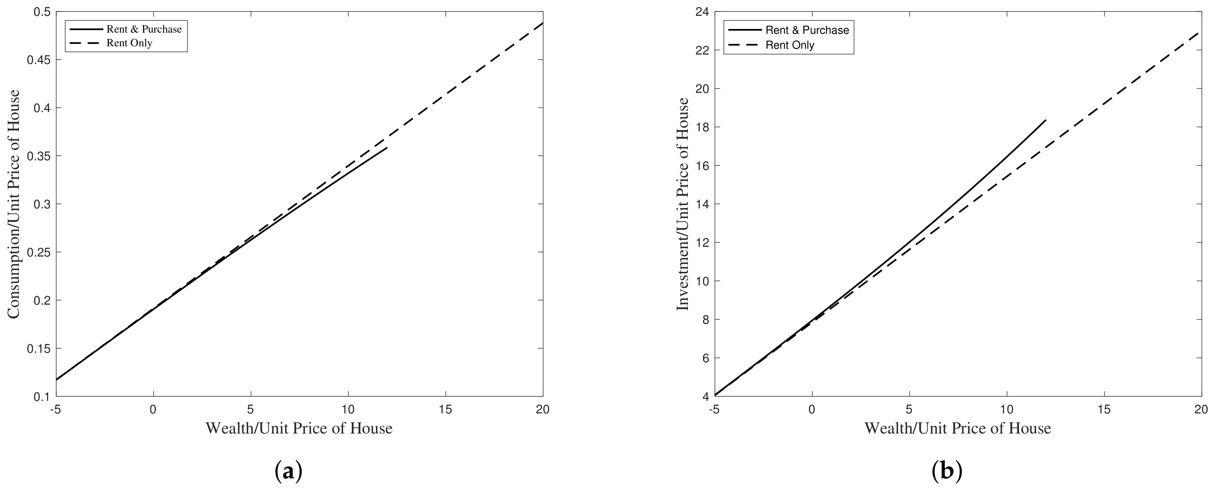
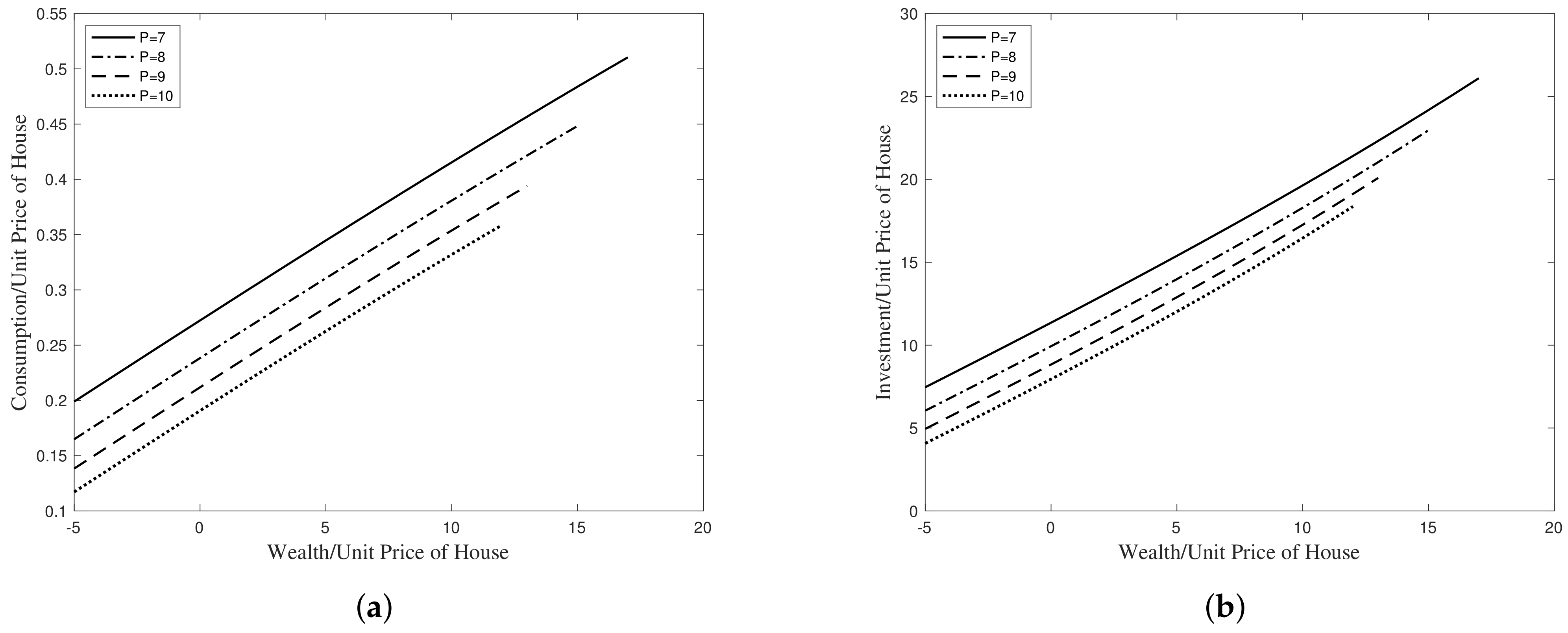
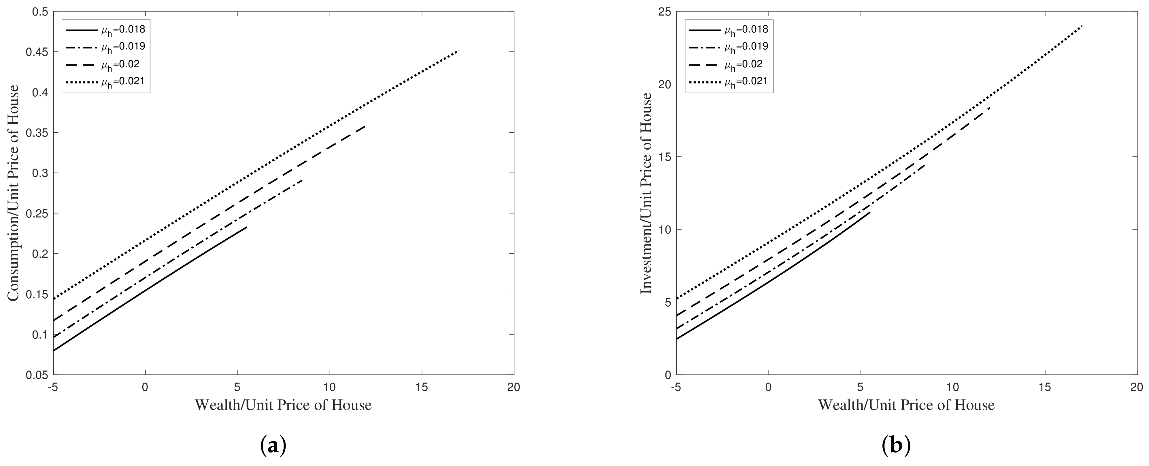
5.2. Consumption and Investment

This subsection analyzes the effects of changes in each parameter on the agent’s optimal consumption and investment policies through numerical figures. As [2,24] indicated, housing choices have a significant impact on a household’s investment in other assets such as stocks and bonds, and should be investigated in deep. However, because the comparative statics and implications of consumption and investment policies have been analyzed in depth in many previous studies, we will only briefly describe them (For detailed analysis, please refer to [6,7,8,9,10,11,12], and references therein). In addition, in all the figures, the consumption and investment after τ p are omitted because they do not have any special additional implications.
First, we present the baseline graphical results to derive the fundamental implications about the consumption and investment choices with the optimal purchasing time for a house in Figure 5.
As the agent’s wealth level approaches X ˜ τ p , the consumption rate is gradually reduced compared to that in the benchmark, the problem with the rent option only. In contrast, the investment is gradually increased. Because the agent in the benchmark has no option to buy a house, they have no need to accumulate capital as their wealth level approaches X ˜ τ p . However, if the agent can purchase a house, because it can be more preferable beyond a certain level of wealth, they begin to reduce consumption and increase investment to buy a house quickly. This result can be regarded as similar to the optimal consumption and investment behavior of agents near their retirement times in most studies on optimal voluntary retirement [6,7].
The following Figure 6 describe the comparative statics on the unit price of a house, P, in relation to the consumption and investment choices. All the parameter values in the following figures are equal to the baseline parameter values in (37), except for P. The results are very trivial. As the house price rises, the rent that the agent has to pay increases, thereby reducing the consumption and investment.
We also present the impact of the expected growth rate of the housing price on the consumption and investment decisions in the following Figure 7. As previously described, when μ h increases and ceteris paribus, because it is similar to paying relatively low housing costs, the agent increases their consumption and investment.
The following Figure 8 demonstrate the relationship between the elasticity of substitution between consumption and housing, α , and the consumption and investment policies. As α becomes larger, the agent obtains a greater utility from consumption, which results in a great increase in consumption. At the same time, the agent buys a house at a smaller financial wealth level because they do not mind living in a smaller house.

6. Conclusions

In this study, we established a housing choice model, which has not been thoroughly investigated in most mathematical portfolio selection problems, and derived its closed-form solution. Specifically, this model is very realistic in describing how an agent chooses the size of the house to live in, and, at the same time, chooses whether to rent or purchase a house. We derived a closed-form solution using a dynamic programming approach, and derived the economic implications of our model using various numerical demonstrations. In particular, we analyzed in depth how the parameters of the financial and housing markets affect individual housing choices.
The limitation of this study is that the real-world behavior of consumers after owning a house is relatively simplified for parsimony, even if households do not trade houses frequently. For example, after purchasing a house, the agent does not consider the option of becoming a lessor while investing in the multiple housing assets. Subsequently, the agent’s choice to inherit the estate to his/her heir is also not reflected. Another limitation of the model is that the stochastic volatility of housing assets and risky assets are not taken into account. Although it is widely known that the volatility of houses or stocks changes over time, we consider a simple constant volatility for parsimony so that we can focus on the optimal stopping time to purchase a house.
Overall, our study makes a great contribution because it extends the mathematical portfolio selection model to a model that deals with housing choices. In particular, the results of this study have various useful points of applications. Due to the recent COVID-19 pandemic, housing prices in many countries have soared, which has brought about a major change in the outlook for future housing price growth. This study can serve as a fundamental study to analyze the impact of these changes on housing demand of sales and rents. It can also provide insight into asset management by providing a foundational model for the relationship between the housing market and other risky investments markets.
It will be relatively easy to extend our model to more diverse housing selection-related models, including those discussed above. For example, it will be possible to study a model that includes borrowing constraints such as loan-to-value ratios or debt-to-income ratios, where an agent selects the optimal housing size based on their age, or a model that considers taxes.

Author Contributions

Conceptualization, S.A.; formal analysis, Q.L.; funding acquisition, S.A.; investigation, Q.L. and S.A.; methodology, Q.L.; project administration, S.A.; software, Q.L.; supervision, S.A.; validation, Q.L. and S.A.; visualization, Q.L.; writing—original draft, Q.L. and S.A.; writing—review and editing, Q.L. and S.A. All authors have read and agreed to the published version of the manuscript.

Funding

This research was funded by the Ministry of Education of the Republic of Korea and the National Research Foundation of Korea (NRF-2021S1A5A2A03063960).

Institutional Review Board Statement

Not applicable.

Informed Consent Statement

Not applicable.

Data Availability Statement

Not applicable.

Conflicts of Interest

The authors declare no conflict of interest.

Appendix A. Detailed Proof of Theorem 2

Applying Lemma 1, the derivatives of the value function V ( x , p ) can be expressed as follows:
V x = p α ( 1 γ ) 1 V ˜ ( x ˜ ) , 2 V x 2 = p α ( 1 γ ) 2 V ˜ ( x ˜ ) , V p = p α ( 1 γ ) 1 α ( 1 γ ) V ˜ V ˜ ( x ˜ ) x ˜ , 2 V p 2 = [ α ( 1 γ ) 1 ] p α ( 1 γ ) 2 α ( 1 γ ) V ˜ 2 V ˜ ( x ˜ ) x ˜ + p α ( 1 γ ) 2 V ˜ ( x ˜ ) x ˜ 2 , 2 V x p = [ α ( 1 γ ) 1 ] p α ( 1 γ ) 2 V ˜ ( x ˜ ) p α ( 1 γ ) 2 V ˜ ( x ˜ ) x ˜ .
Substituting the derivatives above into (21) gives the following equation:
β p α ( 1 γ ) V ˜ = max c , π , h [ { r x ˜ p + ( μ r ) π ˜ p c ˜ p δ p h + I ˜ p } p α ( 1 γ ) 1 V ˜ ( x ˜ ) + 1 2 σ 2 ( π ˜ p ) 2 p α ( 1 γ ) 2 V ˜ ( x ˜ ) + μ h p p α ( 1 γ ) 1 α ( 1 γ ) V ˜ V ˜ ( x ˜ ) x ˜ + 1 2 σ h 2 p 2 ( α ( 1 γ ) 1 ) p α ( 1 γ ) 2 α ( 1 γ ) V ˜ 2 V ˜ ( x ˜ ) x ˜ + p α ( 1 γ ) 2 V ˜ ( x ˜ ) x ˜ 2 + σ σ h ( π ˜ p ) p ( α ( 1 γ ) 1 ) p α ( 1 γ ) 2 V ˜ ( x ˜ ) p α ( 1 γ ) 2 V ˜ ( x ˜ ) x ˜ + ( c ˜ p ) α h 1 α 1 γ 1 γ ] .
Then, reducing and reorganizing (A1) by using η 1 , η 2 , β ˜ and u ( c ˜ , h ) in (23), (24), (16), and (25) respectively, result in (22).
To simplify the notations, we use c ˜ to represent the optimal c ˜ * , π ˜ to represent the optimal π ˜ * , and h to represent the optimal h * . Referring to Definition 1, we set the optimal c ˜ = C ˜ ( x ˜ ) , and X ˜ ( · ) = C ˜ 1 ( · ) , that is, X ˜ ( c ˜ ) = X ˜ ( C ˜ ( x ˜ ) ) = x ˜ . Then, we obtain the following from (27):
V ˜ ( x ˜ ) = η 3 ( 1 γ ) α C ˜ ( x ˜ ) γ ,
V ˜ ( x ˜ ) = γ η 3 ( 1 γ ) α C ˜ ( x ˜ ) γ 1 X ˜ ( c ˜ ) 1 .
Thus, (30) can be derived by plugging (A2) and (A3) into (29).
If we take the derivative of (30) with respect to c ˜ , we obtain the following:
β ˜ η 3 ( 1 γ ) α c ˜ X ˜ ( c ˜ ) = η 1 + σ h η 2 σ X ˜ ( c ˜ ) η 3 ( 1 γ ) α c ˜ η 1 + σ h η 2 σ X ˜ + I ˜ γ η 3 ( 1 γ ) α + ( 1 γ ) c ˜ η 3 γ + 1 2 η 2 2 η 3 ( 1 γ ) 2 α c ˜ X ˜ ( c ˜ ) σ 2 γ + 1 2 η 2 2 η 3 ( 1 γ ) α c ˜ 2 X ˜ ( c ˜ ) σ 2 γ .
Reducing (A4) results in the ODE (31).
For the general solution, we conjecture X ˜ ( c ˜ ) = c ˜ m and substitute it into (31), then we have
X ˜ ( c ˜ ) = A 1 c ˜ γ m + + B 1 c ˜ γ m .
For a particular solution, we conjecture that X ˜ ( c ˜ ) = C 1 c ˜ + D 1 and substitute it into (31). Then, we obtain the following:
C 1 = 1 α K , D 1 = I ˜ r ˜ .
For the solution of X ˜ ( c ˜ ) to be well-defined, we choose A 1 = 0 , and (32) is the closed-form solution of (31).
Taking the first-order condition of (34) with respect to h ¯ , we have
V X τ p ̲ P τ p = V ¯ h ¯ ,
then
α κ 1 γ c τ p α ( 1 γ ) 1 h ¯ ( 1 α ) ( 1 γ ) P τ p = ( 1 α ) ( 1 γ ) h ¯ ( 1 α ) ( 1 γ ) 1 Υ c τ p α ( 1 γ ) .
Furthermore, (35) is given by reorganizing (A6).
From (A2), (35), the first-order condition with respect to c of (11), and the smooth-pasting condition, we obtain
P τ p α ( 1 γ ) 1 η 3 ( 1 γ ) α η c τ p P τ p γ = α κ 1 γ c τ p α ( 1 γ ) 1 ( 1 α ) ( 1 γ ) Υ c τ p α κ 1 γ P τ p ( 1 α ) ( 1 γ ) .
Then, reducing (A7) makes it possible to derive the value of η in (20).

Appendix B. Solution to Problem 3

The closed-form solutions of value function V b ( x , p ) , the optimal consumption rate, the portfolio process, and the housing rate in Problem 3 are given by the following:
V b ( x , p ) = 1 β ˜ p ( 1 α ) ( 1 γ ) α K x + I r ˜ 1 γ η 3 γ + 1 K ( 1 γ ) 1 2 γ θ ˜ 2 + r ˜ , c t * = α K X t + I r ˜ , π t * = σ h σ γ + η 2 σ 2 γ X t + I r ˜ I σ h r ˜ σ , h t * = ( 1 α ) K δ P t X t + I r ˜ .

References

  1. Grossman, S.J.; Laroque, G. Asset Pricing and Optimal Portfolio Choice in the Presence of Illiquid Durable Consumption Goods. Econometrica 1990, 58, 25–51. [Google Scholar] [CrossRef]
  2. Cocco, J.F. Portfolio Choice in the Presence of Housing. Rev. Financ. Stud. 2005, 18, 535–567. [Google Scholar] [CrossRef]
  3. Karatzas, I.; Lehoczky, J.P.; Sethi, S.P.; Shreve, S.E. Explicit Solution of a General Consumption/Investment Problem. Math. Oper. Res. 1986, 11, 261–294. [Google Scholar] [CrossRef]
  4. Merton, R.C. Lifetime Portfolio Selection under Uncertainty: The Continuous-Time Case. Rev. Econ. Stat. 1969, 51, 247–257. [Google Scholar] [CrossRef] [Green Version]
  5. Merton, R.C. Optimum Consumption and Portfolio Rules in a Continuous-Time Model. J. Econ. Theory 1971, 3, 373–413. [Google Scholar] [CrossRef] [Green Version]
  6. Choi, K.J.; Shim, G. Disutility, Optimal Retirement, and Portfolio Selection. Math. Financ. 2006, 16, 443–467. [Google Scholar] [CrossRef]
  7. Farhi, E.; Panageas, S. Saving and Investing for Early Retirement: A Theoretical Analysis. J. Financ. Econ. 2007, 83, 87–121. [Google Scholar] [CrossRef]
  8. Dybvig, P.H.; Liu, H. Lifetime Consumption and Investment: Retirement and Constrained Borrowing. J. Econ. Theory 2010, 145, 885–907. [Google Scholar] [CrossRef] [Green Version]
  9. Lim, B.H.; Shin, Y.H.; Choi, U.J. Optimal Investment, Consumption, and Retirement Choice Problem with Disutility and Subsistence Consumption Constraints. J. Math. Anal. Appl. 2008, 345, 109–122. [Google Scholar] [CrossRef]
  10. Lee, H.-S.; Shin, Y.H. An Optimal Consumption, Investment and Voluntary Retirement Choice Problem with Disutility and Subsistence Consumption Constraints: A Dynamic Programming Approach. J. Math. Anal. Appl. 2015, 428, 762–771. [Google Scholar] [CrossRef]
  11. Choi, K.J.; Shim, G.; Shin, Y.H. Optimal Portfolio, Consumption-Leisure and Retirement Choice Problem with CES Utility. Math. Financ. 2008, 18, 445–472. [Google Scholar] [CrossRef]
  12. Shin, Y.H. Voluntary Retirement and Portfolio Selection: Dynamic Programming Approaches. Appl. Math. Lett. 2012, 25, 1087–1093. [Google Scholar] [CrossRef] [Green Version]
  13. Ahn, S.; Choi, K.J.; Lim, B.H. Optimal Consumption and Investment under Time-Varying Liquidity Constraints. J. Financ. Quant. Anal. 2019, 54, 1643–1681. [Google Scholar] [CrossRef]
  14. Detemple, J.; Serrat, A. Dynamic Equilibrium with Liquidity Constraints. Rev. Financ. Stud. 2003, 16, 597–629. [Google Scholar] [CrossRef]
  15. Duffie, D.; Fleming, W.H.; Soner, H.M.; Zariphopoulou, T. Hedging in Incomplete Markets with HARA Utility. J. Econ. Dyn. Control 1997, 21, 753–782. [Google Scholar] [CrossRef] [Green Version]
  16. El Karoui, N.; Jeanblanc-Picqué, M. Optimization of Consumption with Labor Income. Financ. Stoch. 1998, 2, 409–440. [Google Scholar] [CrossRef]
  17. He, H.; Pagès, H.F. Labor Income, Borrowing Constraints, and Equilibrium Asset Prices. Econ. Theory 1993, 3, 663–696. [Google Scholar] [CrossRef]
  18. Dybvig, P.H. Dusenberry’s Ratcheting of Consumption: Optimal Dynamic Consumption and Investment Given Intolerance for Any Decline in Standard of Living. Rev. Econ. Stud. 1995, 62, 287–313. [Google Scholar] [CrossRef]
  19. Gong, N.; Li, T. Role of Index Bonds in an Optimal Dynamic Asset Allocation Model with Real Subsistence Consumption. Appl. Math. Comput. 2006, 174, 710–731. [Google Scholar] [CrossRef]
  20. Koo, J.L.; Ahn, S.; Koo, B.L.; Koo, H.K.; Shin, Y.H. Optimal Consumption and Portfolio Selection with Quadratic Utility and a Subsistence Consumption Constraint. Stoch. Anal. Appl. 2016, 34, 165–177. [Google Scholar] [CrossRef]
  21. Shin, Y.H.; Koo, J.L.; Roh, K.-H. An Optimal Consumption and Investment Problem with Quadratic Utility and Subsistence Consumption Constraints: A Dynamic Programming Approach. Math. Model. Anal. 2018, 23, 627–638. [Google Scholar] [CrossRef]
  22. Yuan, H.; Hu, Y. Optimal Consumption and Portfolio Policies with the Consumption Habit Constraints and the Terminal Wealth Downside Constraints. Insur. Math. Econ. 2009, 45, 405–409. [Google Scholar] [CrossRef]
  23. Ahn, S.; Ryu, D. The Optimal Chonsei to Monthly-Rent Conversion Choice Given Borrowing Constraints; Working Paper; Pukyong National University: Busan, Korea, 2022. [Google Scholar]
  24. Yao, R.; Zhang, H.H. Optimal Consumption and Portfolio Choices with Risky Housing and Borrowing Constraints. Rev. Financ. Stud. 2005, 18, 197–239. [Google Scholar] [CrossRef]
  25. Yogo, M. Portfolio Choice in Retirement: Health Risk and the Demand for Annuities, Housing, and Risky Assets. J. Monet. Econ. 2016, 80, 17–34. [Google Scholar] [CrossRef] [Green Version]
  26. Flavin, M.; Yamashita, T. Owner-Occupied Housing and the Composition of the Household Portfolio. Am. Econ. Rev. 2002, 92, 345–362. [Google Scholar] [CrossRef]
  27. Chetty, R.; Sándor, L.; Szeidl, A. The Effect of Housing on Portfolio Choice. J. Financ. 2017, 72, 1171–1212. [Google Scholar] [CrossRef]
  28. Nils, C.F.; Bernt, Ø.; Agnès, S. Optimal Consumption and Portfolio in a Jump Diffusion Market with Proportional Transaction Costs. J. Math. Econ. 2001, 35, 233–257. [Google Scholar]
  29. Aït-Sahalia, Y.; Cacho-Diaz, J.; Hurd, T.R. Portfolio Choice with Jumps: A Closed-Form Solution. Ann. Appl. Probab. 2009, 19, 556–584. [Google Scholar] [CrossRef]
  30. Chacko, G.; Viceira, L.M. Dynamic Consumption and Portfolio Choice with Stochastic Volatility in Incomplete Markets. Rev. Financ. Stud. 2005, 18, 1369–1402. [Google Scholar] [CrossRef] [Green Version]
  31. Liu, J. Portfolio Selection in Stochastic Environments. Rev. Financ. Stud. 2006, 20, 1–39. [Google Scholar] [CrossRef]
  32. Lin, M.; SenGupta, I. Analysis of Optimal Portfolio on Finite and Small-Time Horizons for a Stochastic Volatility Market Model. SIAM J. Financ. Math. 2021, 12, 1596–1624. [Google Scholar] [CrossRef]
  33. Hu, Y.; Øksendal, B.; Sulem, A. Optimal Consumption and Portfolio in a Black-Scholes Market Driven by Fractional Brownian Motion. Infin. Dimens. Anal. Quantum Probab. Relat. Top. 2003, 6, 519–536. [Google Scholar] [CrossRef]
  34. Salmon, N.; SenGupta, I. Fractional Barndorff-Nielsen and Shephard Model: Applications in Variance and Volatility Swaps, and Hedging. Ann. Financ. 2021, 17, 529–558. [Google Scholar] [CrossRef]
Figure 1. Optimal housing policies with changes in financial market. (a) Expected return of risky asset, μ . (b) Risk-free rate, r.
Axioms 11 00127 g001
Figure 2. Optimal housing policies with changes in housing price and growth rate of housing price. (a) Unit price of house, P. (b) Expected growth rate of housing price, μ h .
Axioms 11 00127 g002
Figure 3. Optimal housing policies with changes in income rate.
Axioms 11 00127 g003
Figure 4. Optimal housing policies with changes in agent’s preference. (a) Elasticity of consumption/housing, α . (b) Purchasing house preference, κ .
Axioms 11 00127 g004
Figure 5. Comparison of optimal consumption and investment policies between purchasing and rent only. (a) Consumption. (b) Investment.
Axioms 11 00127 g005
Figure 6. Optimal consumption and investment policies with changes in housing price. (a) Consumption. (b) Investment.
Axioms 11 00127 g006
Figure 7. Optimal consumption and investment policies with changes in growth rate of housing price. (a) Consumption. (b) Investment.
Axioms 11 00127 g007
Figure 8. Optimal consumption and investment policies with changes in elasticity of substitution between consumption and housing. (a) Consumption. (b) Investment.
Axioms 11 00127 g008
Publisher’s Note: MDPI stays neutral with regard to jurisdictional claims in published maps and institutional affiliations.

