Abstract
Since the beginning of the COVID-19 pandemic, vaccination has been the main strategy to contain the spread of the coronavirus. However, with the administration of many types of vaccines and the constant mutation of viruses, the issue of how effective these vaccines are in protecting the population is raised. This work aimed to present a mathematical model that investigates the imperfect vaccine and finds the additional measures needed to help reduce the burden of disease. We determine the threshold of disease spread and use stability analysis to determine the condition that will result in disease eradication. We also fitted our model to COVID-19 data from Morocco to estimate the parameters of the model. The sensitivity analysis of the basic reproduction number, with respect to the parameters of the model, is simulated for the four possible scenarios of the disease progress. Finally, we investigate the optimal containment measures that could be implemented with vaccination. To illustrate our results, we perform the numerical simulations of optimal control.
1. Introduction
Since the beginning of the ongoing COVID-19 pandemic, the world has been racing to develop a vaccination that helps protect the populations around the world and bring human life to a normal status. This race to find a vaccine was not only challenged by the fast spread of the disease, but also the high rate of mutation of COVID-19. As a result, we witness many vaccination types with different biotechnological approaches and different efficacy [1]. These efficacies are based on clinical trials that might have some limitations as their samples do not necessarily cover a wide population from different parts of the world. These facts make the question of the efficacy of vaccines legitimate and need to be investigated.
This problem was investigated using mathematical modeling to study the possible measure that needed to be implemented to reduce the impact of an imperfect vaccine.
The mathematical model of the imperfect vaccination of infectious disease was started by the work of Arino et al. [2]. Many papers have followed up on this work, looking into the various spreads of imperfect vaccination for various diseases. For example, the work of Abu-Raddad [3] studied the mathematical model of a possible HIV vaccination where the authors investigated the impact of the defectiveness of vaccination on the progress of the disease. Liu et al. [4] studied a general SIR with an added vaccination compartment and imperfect vaccination. This study showed how vaccination reduced the infected population but could not eradicate the infection. In fact, the eradication required an additional necessary condition. If vaccination efficacy improves, this condition may be alleviated. A mathematical model with the imperfect vaccination of birds in the case of avian influenza was studied in [5]. This model considered age-since-vaccination structure and symptomatically infected birds. This study showed that the only way eradicate the disease was by the full coverage of the bird population or by full efficacy. A time delay model of imperfect vaccination was studied in [6] with a possible loss of immunity. The study showed the existence of the critical vaccination coverage needed to eliminate the infection. In the case of imperfect vaccination, the authors showed that a critical proportion of the population needed vaccination. Another delay model with distributed delay [7] and the delay model with a generalized incidence function were studied in [8].
Regarding the ongoing pandemic, there are some studies that have investigated imperfect vaccination in the USA ([9,10]) and the UK [11] but without finding optimal measures that could help contain the pandemic, as the use of an imperfect vaccine cannot achieve the low endemicity of COVID-19. On the other hand, many studies (see [12,13,14,15,16,17,18,19,20,21,22]) used optimal control to find the optimal way to allocate vaccination and the best strategy to vaccinate the population, depending on the age or comorbidity of the population. The goal of this paper was to investigate a mathematical model of the imperfect vaccination of COVID-19. The aim was to study the dynamics of this model and present the possible control measures that need to be implemented in order to reduce the impact of the vaccine’s imperfection.
To our knowledge, our work is the only one to date to have studied the potential dynamics of imperfect vaccination and the optimal use of other public health measures that help to reduce the effect of administering imperfect vaccination. The only work that combined these two problems was used in the case of possible malaria vaccination [23].
The structure of this paper is summarized as follows. In Section 2, the mathematical model is formed and the existence conditions of the system are verified. Section 3 takes into account the basic reproduction number. Section 4 and Section 5 analyze the local and global stability at the disease-free equilibrium point, respectively. The optimal control problem of vaccination and additional measures to reduce the disease spread are presented in Section 6. In Section 7, we fit our model to data from Morocco to estimate the parameters of the model. We also discussed four possible scenarios of the dynamic of the model via the elasticity of the basic reproduction number and we give the illustration of the optimal solution via numerical simulations. The conclusion and discussion of the results are given in Section 8.
2. The Mathematical Model
Nine epidemiological compartments were recognized in the population: susceptible (S); vaccinated (V); exposed (E) (asymptomatic); infected with mild symptoms (I); quarantined in a home with mild symptoms (Q); hospitalized (H); quarantined in a hospital with complications (C) (i.e., isolated in a hospital with breathing assistance); and mortality due to disease (D):
In this model, we assume that vaccination does not provide complete protection against COVID-19. As a result, the rate of being vaccinated is , and is the rate of vaccinated persons who have recovered and developed immunity. We suppose that each infectious sub-population (E and I) infected the healthy population at varying densities, where is the infection density per capita with . In reality, our major assumption about vaccination’s imperfection is that some vaccinated persons may only receive partial protection and may become sick if they are exposed to multiple infections. The imperfection can be due to the mutation of the virus. In fact, when people are vaccinated, they tend to relax their guard and take fewer protection measures again the virus. is the proportion of infected individuals. Some people show mild symptoms with the per capita rate and can stay at home with treatment; whilst others develop hard symptoms and must be monitored in the hospital with the per capita rate and another critical condition that requires penetrating breathing with per capita rate . The parameter , with , represents the recovery rates of quarantined, hospitalized and critical infected persons (respectively). Average quarantine and hospitalization times are and , respectively. Finally, represents the mortality rate due to disease. The flow chart of the model is given in the Figure 1. When the nine equations in (1) are combined together, the total population size N remains constant.
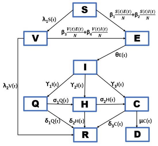
Figure 1.
Flow chart of the model.
2.1. Positivity and Boundedness
This part is dedicated to establishing the positivity and boundedness of the model (1) solutions under non-negative conditions.
Theorem 1.
If , , , , , , and , then the solution , , , , , , , of system (1) is non-negative and the solutions exist in for all .
The proof of positivity follows the standard argument, as can be seen, for example, in [24].
The solution of the model (1) exists in the positively invariant region:
Since all the parameters and sub populations of the system are non-negative and N(t) = constant .
Straightforwardly, we obtain for all . The other variables yielded the same result. As a result, the overall population is finitely upper bounded. For system (1), the region is positively invariant.
2.2. Existence and Uniqueness of Solutions
Theorem 2.
The system (1) that fulfills a given initial condition (, , , , , , , ) has a unique solution.
3. The Basic Reproduction Number
The basic reproduction number is the average number of persons in a susceptible population that one person infected with COVID-19 is expected to infect, and it is calculated using the next generation matrix approach [26]. The disease compartments are thus E and I. Therefore, the all-time disease-free equilibrium point .
The Jacobian matrices of and computed at are provided by F and V, respectively, such that:
The inverse of V is given by
Therefore, the domainant eigenvalue of :
4. Local Stability Analysis at Disease-Free Equilibrium (DFE)
The DFE’s local stability is investigated as follows.
The Jacobian matrix of the system (1) at is:
The eigenvalues of the Jacobian matrix are the roots of the following characteristic equation:
where:
The roots of are given by
with and .
It is straightforward that if and .
In the case for , we write the equation:
From the previous Equation (8), if , then:
Using the same steps as in Equation (8), if , then:
Notice that the fact that implies that and since . Then, we conclude that it is enough to have to ensure that the roots of are negative. On the other hand, if , then . As a result, we have just proven the following theorem:
Theorem 3.
If , the disease-free equilibrium of the system (1) is locally asymptotically stable, but unstable if , where: .
5. Global Stability Analysis at Disease-Free Equilibrium
The global stability of the disease-free equilibrium point was found in this part by creating the Lyapunov function as follows:
Theorem 4.
The disease-free equilibrium of the model (1) is globally asymptotically stable whenever , where .
Proof.
Consider the Lyapunov function L in the trivial equilibrium point , which has non-negative coefficients and :
Differentiating Equation (9) with respect to time t, and substituting both and from Equation (1) yields the result:
By simplifying Equation (10) by collecting similar terms of E and I, then by solving for coefficient and , this yields:
where , .
Since , then . Therefore, is negative if . Furthermore, if and only if . It can thus be investigated whether singleton is the highest compact invariant set for the model (1). Thus, by LaSalle’s invariance principle [27], the DFE is globally asymptotically stable in a region around . □
Remark 1.
The above result shows that and can be reduced to less than a unit so that the disease disappears. Obviously, means that if , then the complete eradication of disease is guaranteed.
6. The Optimal Imperfect Vaccination
When imperfect vaccination is administered to a population, there is a need to find the optimal approach to use it in order to reduce the burden of the disease in the population. The goal of this section is to implement the best control strategy possible in the situation of an imperfect vaccination. Three types of control are used for this purpose. First, the control represents the awareness of taking the vaccine via media, as well as creating knowledge of the positive effects of vaccination to gain herd immunity in the population. The second control is the movement restrictions for susceptible and vaccinated individuals by adhering to a preventative protocol, avoiding the exposure of the vaccinated people to the coronavirus via non-pharmaceutical measures. The third one seeks to improve the efficacy of the vaccine.
Therefore, the model with control strategies is given by
With:
and is a set of admissible controls defined by
The objective function to minimize is:
The positive weight constants , and , respectively, keep the sizes of , , and in balance. Positive weight parameters: , , and are related with the controls , , and in the objective functional.
To solve the problem, we first compute the Lagrangian and Hamiltonian. Equation (16) in order to identify an optimal solution. The optimal problem’s Lagrangian is:
For the control problem, we may define the Hamiltonian as follows:
where are the adjoint functions to be found.
We have the existence result:
Theorem 5.
Proof.
We use the result [28] to show that an optimal control exists. The control and the state variables are both non-negative. This minimization problem satisfies the convexity requirement of the objective functional.
The control space previously defined as (15) is both convex and closed by definition. In order for the optimal control to exist, it is necessary for the optimal system to be compact. The boundedness of the optimal system determines the compactness needed. Additionally, an integrand throughout the functional (16) is convex on the control . It can be concluded that the constant exists, as do positive integers , and such that . This leads us to conclude that optimal control exists. □
Characterization of the Optimal Control
We then investigate the necessary optimal control conditions. For this purpose, the maximum principle of Pontryagin to Hamiltonian [29] can be applied.
Theorem 6.
Let , , , , , , , and represent optimal state solutions with optimal control variables for the optimal control problem (16). are thus adjoint variables that satisfy:
Conditions of transversality.
Moreover, the optimal control is provided by
Proof.
By using Hamiltonian (18), Pontryagin’s maximum principle and setting , , , , , , , and to obtain the following:
Using optimality conditions, we conclude that:
Hence:
By applying the control space property, we obtain that:
which means that:
Since:
We have:
Thus, optimal control is defined as
□
7. Numerical Simulation
The goal of this section is to show how the control strategies can be used to improve outcomes in vaccination campaigns in Morocco. After fitting the model to the data, the estimated parameters are taken to perform sensitivity analysis and determine the optimal control.
7.1. Parameter Estimation
We used data from a vaccination campaign in Morocco between 1 February 2021 and 25 March 2021 to validate our findings. We consider the data from the COVID-19 data [30] and the initial conditions within the values of available data on 1 February 2021 are = (36,202,000, 200,081, 25,543, 13,099, 9824, 1572, 131, 450,052, 8287). These initial values were estimated from the data, apart from and , which were assumed. To obtain the best fitting curve for actual data, we applied the least-squares fitting technique [31]. The parameter values of the model are estimated based on this fitting and are given as follows: , , , , , , , , , , , , , , and . The value of the basic reproduction number in this case is . The fit of the number of individuals infected with COVID-19 in Morocco is described in Figure 2.
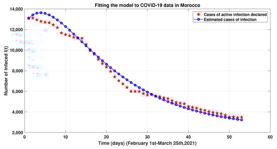
Figure 2.
Fitting the infected population with real data from 1 February 2021 to 25 March 2021.
7.2. Sensitivity Analysis
In this part, we aimed to study the sensitivity of the model parameters with respect to . The goal is to determine the impact of these parameters on the endemicity of the disease. The sensitivity analysis for this outbreak threshold demonstrates the importance of each parameter in the spread of COVID-19, allowing us to determine which parameter to make more sensitive on with respect to a specific parameter, , via the sensitivity index define by
Using the previous definition:
Each parameter’s sensitivity index, corresponding to the basic reproductive numbers , was computed and displayed in Table 1, and the graphical bar-graph findings were generated in Figure 3. The sensitivity indices indicate the importance of each parameter in disease transmission and prevalence. These are some examples: if , it means that if went up (or decreased) by 93.1%, is also likely to increase or decrease by 93.1%. Similarly, for , the decrease in the parameter by 82.02% will fall (or increase ) by a similar proportion.

Table 1.
Sensitivity index for each parameter that has a direct correlation to .
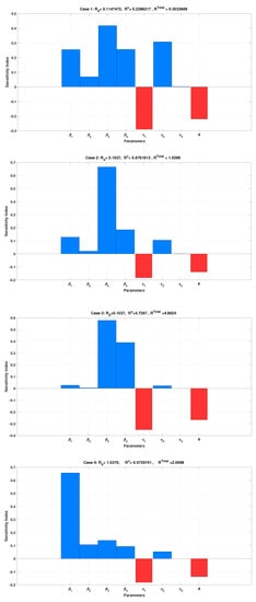
Figure 3.
Scenarios of sensitivity respecting the parameters.
Our goal is to simulate the elasticity of with respect to model parameters in four scenarios that represent the different scenarios of the dynamics of the model as follows:
- Scenario 1: There is no disease persistence (, and ).
- Scenario 2: Persistence of diseases with low threshold values (, and ).
- Scenario 3: The disease persists, with a high endemicity among vaccinated people and a low endemicity among non-vaccinated people (, and ).
- Scenario 4: The disease persists, with low endemicity among the vaccinated and high endemicity among the unvaccinated (, and ).
All of the sensitivity scenarios described above demonstrate that the basic reproductive number is more sensitive to some parameters than others—particularly in the cases of , , and . Scenario 1 has no persistent disease, but Scenario 3 has persistent disease with significant endemicity among the vaccinated, as can be seen from the sensitivity indices of (rate of infected getting isolated) and (incubation period). The same observation applies to the scenarios of the persistence of disease with low endemicity in Scenario 2 and the persistence of disease with high endemicity among the vaccinated in Scenario 4. The level of sensitivity of these parameters is higher when endemicity is low among the non-vaccinated population. Our simulations revealed that the value of the sensitivity index changes depending on the Scenarios (1, 2, 3, 4), with being the highest value for Scenarios 1 and 2. However, in , we can see more domination for the index in Scenario 4.
7.3. Simulation of Optimal Control
The time series of variables in the model without and with optimal control are shown in the figures below. The goal is to compare the effect of control on the different variables of the model.
The three variables are shown in Figure 4: susceptible, infected and recovered without and with optimal control effect. These simulations show that optimal control increases the number of susceptible and recovered people while decreasing the number of infected individuals. The effect of control on the susceptible and recovered populations is obviously more significant since the susceptible and recovered populations rose four-fold in 50 days while the infected population declined by one fold during the same period. This means that the control is very effective for all of these three compartments.
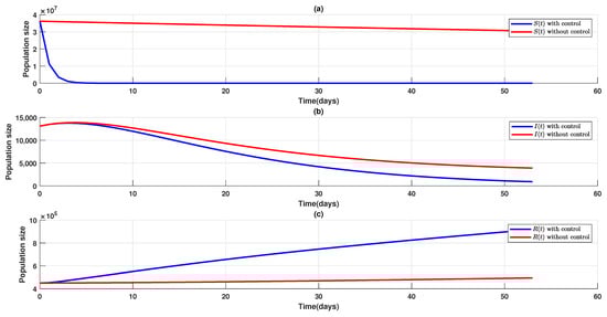
Figure 4.
Time series of the states S, I and R without and with control.
The simulation of the time series of the variables representing the vaccinated, exposed and deceased individuals is shown in Figure 5. Clearly, the vaccinated population benefits more from the optimal control than the exposed population since the control aims to improve vaccination effectiveness. The control strategy, on the other hand, has no obvious effect on the number of deaths.
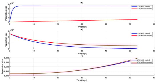
Figure 5.
The time series of states V, E and D without and with control.
Similarly, as seen in Figure 6, the control strategy reduces the number of isolated populations (at home or in hospital). However, there is more benefit to controlling the population with mild symptoms compared to people in the hospital with severe or critical symptoms. When applying the control to all three categories of quarantined, hospitalized, and critical cases of COVID-19, it is clear that the control is obvious.
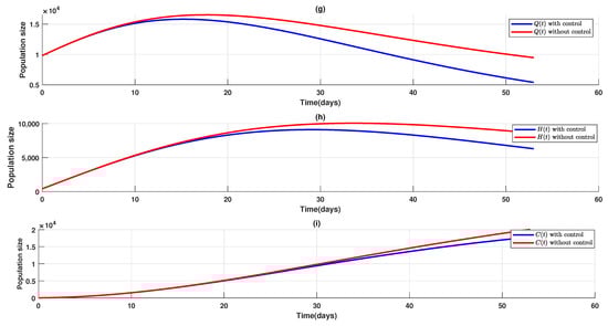
Figure 6.
Time series of the states Q, H and C with and without control.
The three types of optimal controls are given in Figure 7, Figure 8 and Figure 9. Those figures show the intensity of each measure needed to be implemented in the case of imperfect vaccination. The awareness campaign should stay as long as 7 weeks with maximum intensity. At the same time, non-pharmaceutical measures must take place, including mobility restrictions or lockdown for at least 24 days. With regard to the third control measure, the improvement of the vaccine population should increase to reach possible efficacy during the first week of vaccination and stay above within the first 50 days of vaccination. The outcome of this control approach shows that these three measures must be simultaneously implemented to deal with imperfect vaccination.
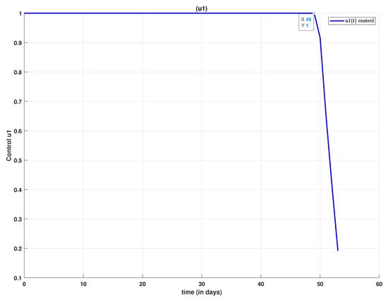
Figure 7.
Evolutionary dynamics of the control .
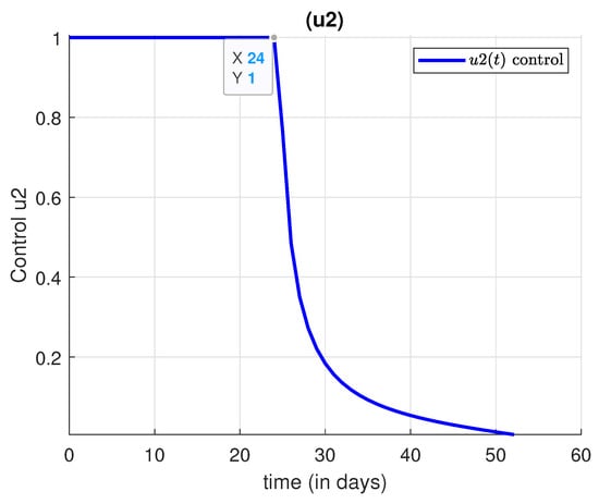
Figure 8.
Evolutionary dynamics of the control .
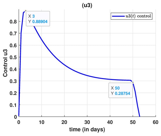
Figure 9.
Evolutionary dynamics of the control .
8. Conclusions
COVID-19 is still taking a toll on people’s lives all over the world. Countries are rushing to implement the vaccination to gain herd immunity, to contain the spread of the disease, and to bring the fatality rate of the disease to the lowest possible level. However, the administered vaccines have different levels of efficacy among the same population, which means the idea of relying on vaccination alone to control the pandemic would not provide total protection for the population against further waves of COVID-19. In this work, we aimed to present a mathematical model of the imperfect vaccination of COVID-19 and to study the dynamics of this model. One further element of this model is that susceptible and vaccinated people have different infection rates and the fatality rate of the disease (rate of death due to the infection) is related to the percentage of the isolated population that is in critical condition. We derive a threshold which is the basic reproduction number of disease transmission among the population. We showed that this threshold does not give us sharp epidemiological properties of the model. In fact, we prove, via the Lyapunov method, that the disease is globally asymptotically stable if with is the sum of and , which is the threshold of transmission of the disease among the vaccinated population. This finding shows that the increase in the efficacy of the vaccination should lead to protecting the population from infection (low and ) which will help control the pandemic.
To make our analysis more realistic, we estimated the parameters of our model using data from Morocco between 1 February 2021 and 25 March 2021. Within the range of the estimated parameters, we performed a sensitivity analysis of with respect to the parameters of the model to find the elasticity index with respect to each parameter. Depending on the disease status, our simulation (Figure 3) produced four outcomes. Scenario 1: There is no disease persistence. Scenario 2: Persistence of diseases with low threshold values. Scenario 3: The disease persists with a high endemicity among vaccinated people and a low endemicity among non-vaccinated people. Scenario 4: The disease persists, with low endemicity among the vaccinated and high endemicity among the unvaccinated.
To further investigate the possible additional measures that help with vaccination. We introduce an optimal control problem with the goal of increasing the awareness of vaccination, limiting the probability of infection by adhering to a preventative protocol and increasing the efficacy of the vaccine. The public health authorities can easily implement these measures. In fact, as the virus mutates, many governments are pushing their populations to get vaccinated and asking people to reduce their contact and wear masks. Moreover, there is a constant effort to increase the efficacy of the vaccine by producing new ones or by boosters.
Our solution of optimal control showed that, to reduce the impact of imperfect vaccination, we needed a longer awareness campaign to engage the population in vaccination. On the other hand, the restriction on population mobility should not be long, since our simulation showed a drop of from 1 (full restriction) after 24 days. To ensure the full protection of the health population, vaccination efficacy must increase by in the first 50 days.
In conclusion, our work showed that facing the imperfection of the vaccination of COVID-19, we mainly have to focus on two measures. The first one is to increase awareness of the importance of vaccination, which will increase the number of people vaccinated. The second is to work on developing vaccines with high efficacy that give more protection to the population instead of making the symptoms of viruses less severe. With these two measures, our study showed that population mobility restrictions have the lowest impact on controlling the virus spread.
Author Contributions
Conceptualization, L.B. and A.T.; methodology, M.L. and A.T.; software, L.B. and M.L.; validation, A.T., M.L. and O.Z.; formal analysis, L.B. and A.T.; investigation, L.B.; resources, M.L. and M.R.; data curation, L.B. and M.R.; writing—original draft preparation, L.B. and A.T.; writing—review and editing, L.B. and A.T.; visualization, L.B. and M.L.; supervision, M.L., A.T. and M.R. All authors have read and agreed to the published version of the manuscript.
Funding
This research received no external funding.
Acknowledgments
The authors would like to thank the reviewers for their comments and inputs that help improve the quality of our work.
Conflicts of Interest
The authors declare no conflict of interest.
References
- Corey, L.; Mascola, J.R.; Fauci, A.S.; Collins, F.S. A strategic approach to COVID-19 vaccine R&D. Science 2020, 368, 948–950. [Google Scholar] [PubMed]
- Arino, J.; Cooke, K.; Van Den Driessche, P.; Velasco-Hernández, J. An epidemiology model that includes a leaky vaccine with a general waning function. Discret. Contin. Dyn. Syst.-B 2004, 4, 479. [Google Scholar] [CrossRef]
- Abu-Raddad, L.J.; Boily, M.C.; Self, S.; Longini, I.M., Jr. Analytic insights into the population level impact of imperfect prophylactic HIV vaccines. JAIDS J. Acquir. Immune Defic. Syndr. 2007, 45, 454–467. [Google Scholar] [CrossRef] [PubMed]
- Liu, X.; Takeuchi, Y.; Iwami, S. SVIR epidemic models with vaccination strategies. J. Theor. Biol. 2008, 253, 1–11. [Google Scholar] [CrossRef] [PubMed]
- Gulbudak, H.; Martcheva, M. A structured avian influenza model with imperfect vaccination and vaccine-induced asymptomatic infection. Bull. Math. Biol. 2014, 76, 2389–2425. [Google Scholar] [CrossRef] [PubMed]
- Al-Darabsah, I. Threshold dynamics of a time-delayed epidemic model for continuous imperfect-vaccine with a generalized nonmonotone incidence rate. Nonlinear Dyn. 2020, 101, 1281–1300. [Google Scholar] [CrossRef] [PubMed]
- Djilali, S.; Bentout, S. Global dynamics of SVIR epidemic model with distributed delay and imperfect vaccine. Results Phys. 2021, 25, 104245. [Google Scholar] [CrossRef]
- Al-Darabsah, I. A time-delayed SVEIR model for imperfect vaccine with a generalized nonmonotone incidence and application to measles. Appl. Math. Model. 2021, 91, 74–92. [Google Scholar] [CrossRef] [PubMed]
- Iboi, E.A.; Ngonghala, C.N.; Gumel, A.B. Will an imperfect vaccine curtail the COVID-19 pandemic in the US? Infect. Dis. Model. 2020, 5, 510–524. [Google Scholar] [PubMed]
- Mancuso, M.; Eikenberry, S.E.; Gumel, A.B. Will vaccine-derived protective immunity curtail COVID-19 variants in the US? Infect. Dis. Model. 2021, 6, 1110–1134. [Google Scholar] [CrossRef]
- Webb, G. A COVID-19 Epidemic Model Predicting the Effectiveness of Vaccination in the US. Infect. Dis. Rep. 2021, 13, 62. [Google Scholar] [CrossRef] [PubMed]
- Libotte, G.B.; Lobato, F.S.; Platt, G.M.; Neto, A.J.S. Determination of an optimal control strategy for vaccine administration in COVID-19 pandemic treatment. Comput. Methods Programs Biomed. 2020, 196, 105664. [Google Scholar] [CrossRef] [PubMed]
- Olivares, A.; Staffetti, E. Optimal control-based vaccination and testing strategies for COVID-19. Comput. Methods Programs Biomed. 2021, 211, 106411. [Google Scholar] [CrossRef] [PubMed]
- Shim, E. Optimal allocation of the limited COVID-19 vaccine supply in South Korea. J. Clin. Med. 2021, 10, 591. [Google Scholar] [CrossRef] [PubMed]
- Choi, W.; Shim, E. Vaccine Effects on Susceptibility and Symptomatology Can Change the Optimal Allocation of COVID-19 Vaccines: South Korea as an Example. J. Clin. Med. 2021, 10, 2813. [Google Scholar] [CrossRef] [PubMed]
- Jordan, E.; Shin, D.E.; Leekha, S.; Azarm, S. Optimization in the Context of COVID-19 Prediction and Control: A Literature Review. IEEE Access 2021, 9, 130072–130093. [Google Scholar] [CrossRef]
- Viana, J.; van Dorp, C.H.; Nunes, A.; Gomes, M.C.; van Boven, M.; Kretzschmar, M.E.; Veldhoen, M.; Rozhnova, G. Controlling the pandemic during the SARS-CoV-2 vaccination rollout. Nat. Commun. 2021, 12, 3674. [Google Scholar] [CrossRef] [PubMed]
- Matrajt, L.; Eaton, J.; Leung, T.; Brown, E.R. Vaccine optimization for COVID-19: Who to vaccinate first? Sci. Adv. 2021, 7, eabf1374. [Google Scholar] [CrossRef] [PubMed]
- Choi, Y.; Kim, J.S.; Kim, J.E.; Choi, H.; Lee, C.H. Vaccination Prioritization Strategies for COVID-19 in Korea: A Mathematical Modeling Approach. Int. J. Environ. Res. Public Health 2021, 18, 4240. [Google Scholar] [CrossRef] [PubMed]
- Makhoul, M.; Ayoub, H.H.; Chemaitelly, H.; Seedat, S.; Mumtaz, G.R.; Al-Omari, S.; Abu-Raddad, L.J. Epidemiological impact of SARS-CoV-2 vaccination: Mathematical modeling analyses. Vaccines 2020, 8, 668. [Google Scholar] [CrossRef] [PubMed]
- Wagner, C.E.; Saad-Roy, C.M.; Morris, S.E.; Baker, R.E.; Mina, M.J.; Farrar, J.; Holmes, E.C.; Pybus, O.G.; Graham, A.L.; Emanuel, E.J.; et al. Vaccine nationalism and the dynamics and control of SARS-CoV-2. medRxiv 2021, 373, eabj7364. [Google Scholar] [CrossRef] [PubMed]
- Piraveenan, M.; Sawleshwarkar, S.; Walsh, M.; Zablotska, I.; Bhattacharyya, S.; Farooqui, H.H.; Bhatnagar, T.; Karan, A.; Murhekar, M.; Zodpey, S.; et al. Optimal governance and implementation of vaccination programmes to contain the COVID-19 pandemic. R. Soc. Open Sci. 2021, 8, 210429. [Google Scholar] [CrossRef] [PubMed]
- Mohammed-Awel, J.; Numfor, E.; Zhao, R.; Lenhart, S. A new mathematical model studying imperfect vaccination: Optimal control analysis. J. Math. Anal. Appl. 2021, 500, 125132. [Google Scholar] [CrossRef]
- Thieme, H.R. Princeton series in theoretical and computational biology. In Mathematics in Population Biology; Princeton University Press: Princeton, NJ, USA, 2003. [Google Scholar]
- Birkhoff, G.; Rota, G. Ordinary Differential Equations; John Wiley & Sons: Hoboken, NJ, USA, 1989. [Google Scholar]
- Van den Driessche, P.; Watmough, J. Reproduction numbers and sub-threshold endemic equilibria for compartmental models of disease transmission. Math. Biosci. 2002, 180, 29–48. [Google Scholar] [CrossRef]
- LaSalle, J. Stability theory for ordinary differential equations. J. Differ. Equ. 1968, 4, 57–65. [Google Scholar] [CrossRef] [Green Version]
- Fleming, W.; Rishel, R. Stochastic Differential Equations and Markov Diffusion Processes. In Deterministic and Stochastic Optimal Control; Springer: Berlin/Heidelberg, Germany, 1975; pp. 106–150. [Google Scholar]
- Lee, D.; Milroy, I.P.; Tyler, K. Application of Pontryagin’s maximum principle to the semi-automatic control of rail vehicles. In Proceedings of the Second Conference on Control Engineering, Newcastle, UK, 25–27 August 1982; pp. 233–236. [Google Scholar]
- Roser, M.; Ritchie, H.; Ortiz-Ospina, E.; Hasell, J. Coronavirus Pandemic (COVID-19). Our World in Data. 2022. Available online: https://ourworldindata.org/coronavirus (accessed on 15 January 2022).
- Weisstein, E.W. Least Squares Fitting. 2002. Available online: https://mathworld.wolfram.com/ (accessed on 15 January 2022).
Publisher’s Note: MDPI stays neutral with regard to jurisdictional claims in published maps and institutional affiliations. |
© 2022 by the authors. Licensee MDPI, Basel, Switzerland. This article is an open access article distributed under the terms and conditions of the Creative Commons Attribution (CC BY) license (https://creativecommons.org/licenses/by/4.0/).