Article

Accurate Time-Domain Modeling of Arbitrarily Shaped Graphene Layers Utilizing Unstructured Triangular Grids

by
Stamatios Amanatiadis
1,*,
Theodoros Zygiridis
2 and
Nikolaos Kantartzis
1
1
Department of Electrical & Computer Engineering, Aristotle University of Thessaloniki, GR-54124 Thessaloniki, Greece
2
Department of Electrical & Computer Engineering, University of Western Macedonia, GR-50100 Kozani, Greece
*
Author to whom correspondence should be addressed.
Axioms 2022, 11(2), 44; https://doi.org/10.3390/axioms11020044
Submission received: 7 December 2021 / Revised: 17 January 2022 / Accepted: 19 January 2022 / Published: 22 January 2022
(This article belongs to the Special Issue Advances in Finite-Difference Time-Domain Methods and Applications)

Abstract

:
The accurate modeling of curved graphene layers for time-domain electromagnetic simulations is discussed in the present work. Initially, the advanced properties of graphene are presented, focusing on the propagation of strongly confined surface plasmon polariton waves at the far-infrared regime. Then, the implementation of an unstructured triangular grid was examined, based on the Delaunay triangulation method. The electric-field components were placed at the edges of the triangles, while two different techniques were proposed for the sampling of the magnetic ones. Specifically, the first one suggests that the magnetic component is placed at the triangle’s circumcenter providing more accurate results, although instability may occur for nonacute triangles. On the other hand, the magnetic field was sampled at the triangle’s centroid, considering the second technique, ensuring the algorithm’s stability, but further approximations were required, leading to a slight accuracy reduction. Moreover, the updating equations in the time-domain were extracted via an appropriate approximation of Maxwell equations in their integral form. Finally, graphene was introduced in the computational domain as an equivalent surface current density, whose location matches the corresponding electric components. The validity of our methodology was successfully performed via the comparison of graphene surface wave propagation properties to their theoretical values, whereas the global error determination indicates the minimal triangle dimensions. Additionally, an instructive setup comprising a circular graphene scatterer was analyzed thoroughly, to reveal our technique’s advantages compared to the conventional staircase discretization.

1. Introduction

In previous years, graphene attracted rapid scientific attention due to its extraordinary properties in a broad field of applications. Particularly, this naturally two-dimensional carbon allotrope presents significant and useful characteristics, in spite of its negligible thickness [1]. From an electromagnetic point of view, a finite surface conductivity is observed, thus enabling several exotic phenomena, such as gyrotropy and the propagation of strongly confined surface plasmon polariton (SPP) waves at the far-infrared frequencies [2,3,4]. The latter paved the way for the design of a wide class of plasmonic devices at the THz regime [5,6,7,8].
The majority of these devices require efficient simulation techniques for their precise characterization. Therefore, the development of suitable numerical algorithms that model graphene accurately has been triggered. A very popular numerical scheme is the finite-difference time-domain (FDTD) technique, which facilitates broadband simulations of complex structures [9] owing to its explicit time-domain nature. For this reason, several algorithms have been reported that modify the conventional FDTD method properly, while open-source implementations are available [10]. In general, graphene is treated as a surface boundary, and its inherent frequency dispersion can be modeled through an auxiliary differential equation [11,12] or by exploiting the magnetic-field boundary conditions [13]. Additionally, more advanced properties have been implemented, such as the case of magnetically biased graphene [14,15,16], its third-order response [17,18], and its complex conductivity at optical frequencies [19,20]. Despite its apparent flexibility, the main drawback of the original FDTD algorithm is the discretization of the computational domain with a structured orthogonal mesh. On the other hand, it should be kept in mind that various devices feature optimized designs exploiting curved surfaces. As a consequence, an extremely fine mesh is required for the staircase approximation of such configurations [21,22,23], which degrades the simulation’s performance. Alternatively, frequency-domain numerical solvers can be employed [24,25,26,27], sacrificing the advantages of time-domain solutions.
In this paper, we propose the accurate numerical modeling of arbitrarily shaped graphene layers in the time domain via the discretization of the computational space with unstructured triangular meshes. The analysis starts with the presentation of graphene main attributes, such as its surface conductivity and the fundamental propagation properties of the supported SPP waves. Furthermore, the basic aspects of the unstructured triangular grids were investigated for time-domain electromagnetic simulations. Specifically, two different sampling techniques for the magnetic components were examined, at the triangle circumcenter and at its centroid, while the electric components were placed at the edges of the triangles. Then, the graphene contribution is introduced as an equivalent surface current density, while a recursive convolution method (RCM) was developed for the consistent modeling of its frequency dispersion. The proposed algorithm was successfully validated through the direct comparison of the numerically extracted SPP wave propagation properties with the analytical values, while the global error calculation indicated certain discretization limitations. Finally, an interesting configuration that includes a circular graphene scatterer was designed, and the comparison with the conventional staircase approximation highlighted the superiority of the unstructured grids, in case of problems with nonorthogonal features.

2. Theoretical Formulation

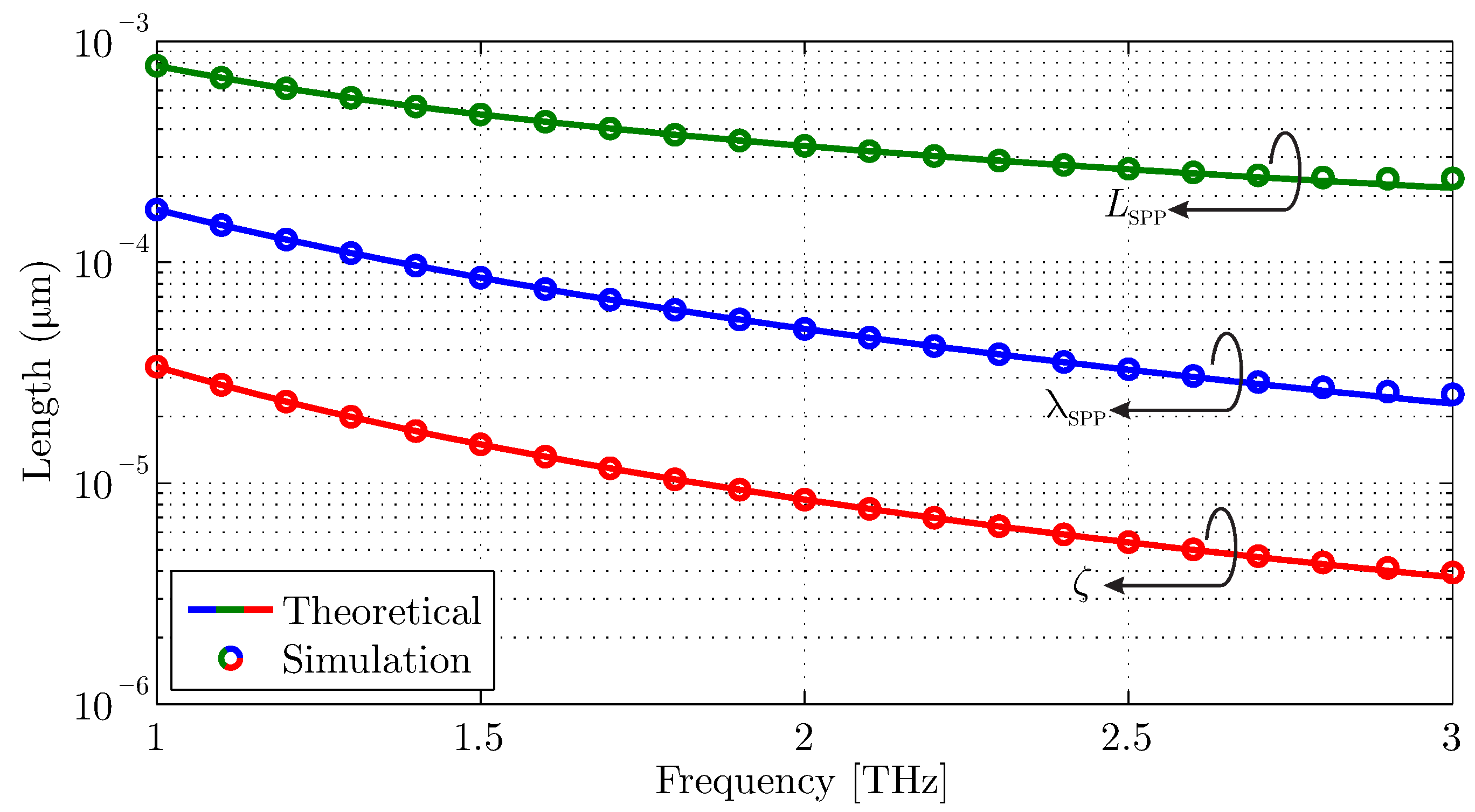
2.1. Graphene Surface Conductivity and Surface Wave Propagation Properties

Throughout this work, graphene is considered to be a naturally infinitesimally thin material, characterized via its surface conductivity σ gr ( ω , μ c , Γ , T ) . The latter depends on the radial frequency ω , the chemical potential μ c that can be controlled either via chemical doping or an electrostatic bias application, the scattering rate Γ that constitutes the main loss mechanism of the material, and the temperature T. Graphene’s surface conductivity is evaluated utilizing the Kubo formula [28], leading to the following compact expression in the absence of an external magnetostatic field [29]:
σ gr ( ω , μ c , Γ , T ) = e 2 ( j ω + 2 Γ ) π 2 × 1 ( j ω + 2 Γ ) 2 0 ε f d ( ε ) ε f d ( ε ) ε d ε + 0 f d ( ε ) f d ( ε ) ( j ω + 2 Γ ) 2 + 4 ( ε / ) 2 d ε ,
where e is a single electron charge, the reduced Planck’s constant and f d ( ε ) is the Fermi–Dirac distribution
f d ( ε ) = 1 ( e ( ε μ c ) / k B T + 1 ) ,
with k B the Boltzmann’s constant. It is evident that (1) consists of two terms that are connected to the major electron transitions in graphene, namely the intraband and the interband. The former dominates at lower frequencies, approximately until the far-infrared regime, while the latter becomes considerable beyond the mid-infrared frequencies. Although the proposed methodology can be extended to incorporate more complex graphene properties, we focus on the lower regime, where the interband term is negligible. Consequently, the graphene’s surface conductivity expression can be significantly simplified to a Debye dispersion relation:
σ gr , intra ( ω , μ c , Γ , T ) = e 2 k B T π 2 ( j ω + 2 Γ ) μ c k B T + 2 ln ( e μ c / k B T + 1 ) = A μ c j ω + 2 Γ ,
where A μ c is the frequency-independent term. It is important to mention that isotropic graphene conductivity is considered instead of the anisotropic one since our analysis is performed for a two-dimensional computational domain.
The capability of graphene to support strongly confined SPP waves at the far-infrared regime is well established. The propagation properties of such waves depend on graphene’s surface conductivity, and their characterization can be performed via the propagation constant k ρ . The latter has been evaluated analytically for a free-standing graphene layer of infinite dimensions by means of [29]
k ρ = k 0 1 2 σ gr η 0 2 ,
where k 0 and η 0 are the free-space wavenumber and wave impedance, respectively. Now, the main propagation attributes, such as the SPP wavelength λ SPP , the propagation length L SPP and the confinement ζ , were straightforwardly extracted from the propagation constant k ρ via
λ SPP = 2 π { k ρ } , L SPP = 1 2 { k ρ } , ζ = 1 k ρ 2 k 0 2 ,
with { · } and { · } denoting the real and the imaginary part of the argument, respectively.

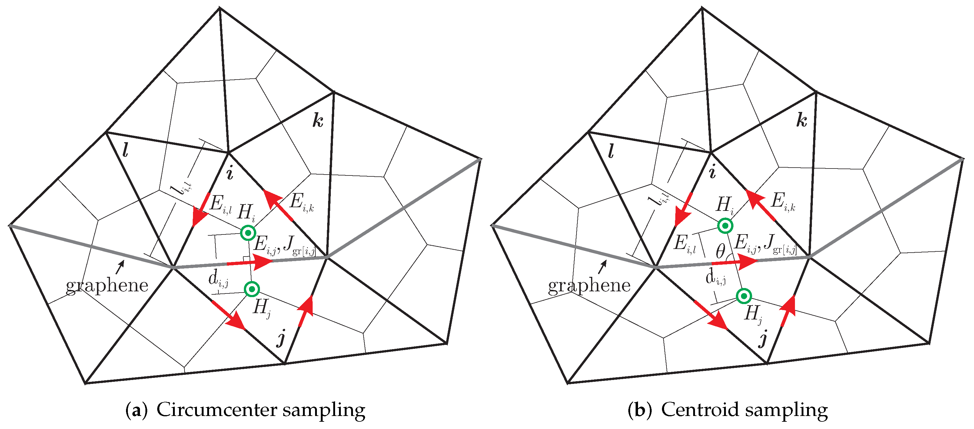
2.2. Unstructured Triangular Grids for Electromagnetic Analysis in the Time Domain

The FDTD approach constitutes one of the most popular methods for electromagnetic simulations in the time domain [30]. The conventional algorithm solves the differential form of Maxwell equations by applying a finite-difference scheme on a structured rectangular grid. Despite the algorithm’s powerful characteristics, the use of a rectangular grid enforces staircase approximations to curved interfaces, which may lead to inaccurate results. For this reason, unstructured triangular grids have been proposed to effectively model such surfaces [31,32]. In our approach, the integral form of Maxwell equations is utilized for isotropic media
C E · d l = A μ 0 μ r H t · d A ,
C H · d l = A ε 0 ε r E t + σ E · d A ,
where A is the area limited by the closed-loop C with length l, ε 0 and μ 0 are the electric permittivity and magnetic permeability of free-space, respectively, and ε r , μ r are their relative equivalents.
Our work focuses on a transverse electric two-dimensional (2D) case. The computational domain is discretized into triangular elements using an efficient Delaunay triangulation algorithm, as depicted in Figure 1. Here, the electric-field components are tangential to the 2D domain and located along the edges of the triangles. It should be mentioned that the sampling of the magnetic components, which are considered normal to the domain, is not a trivial issue. In particular, two different approaches, depicted in Figure 1, are investigated.
The initial one (Figure 1a) places the magnetic components at the triangle circumcenter, namely the center of the circle that is defined by its vertices creating thus, a Voronoi diagram [31]. The advantage of this approach is that the magnetic-field connection between two adjacent triangles is perpendicular to their common edge. This is important, since the inner product at the right-hand side of (7) suggests that the electric component is vertical to the virtual area of the connecting magnetic fields. Unfortunately, these points may lie outside the element for an obtuse triangle case, potentially influencing the algorithm’s stability.
To circumvent this hindrance, a second technique can be used (Figure 1b), where the magnetic components are located at the triangle centroid, namely the averaged coordinates of its three vertices [32]. Although this approach ensures that each magnetic component lies inside the corresponding element, the magnetic-field connection between adjacent triangles is not necessarily vertical to the common electric component. Hence, an angular correction is required for the accurate implementation of (7). Note that the two techniques are identical for the case of equilateral triangles. In this manner, an optimal triangulation can be considered to consist of such elements.
Now, a finite integration was applied to (6) and (7). First of all, the temporal discretization of fields was defined to coincide with the conventional FDTD algorithm, i.e., E was updated at n Δ t and H at ( n + 1 / 2 ) Δ t instants, where Δ t is the time-step. Then, considering element i, (6) was developed into
E i , j n l i , j + E i , k n l i , k + E i , l n l i , l = μ 0 μ r H i n + 1 / 2 H i n 1 / 2 Δ t A , H i n + 1 / 2 = H i n 1 / 2 Δ t A i μ 0 μ r ( E i , j n l i , j + E i , k n l i , k + E i , l n l i , l ) .
The finite integration of (7) depends on the applied magnetic field component sampling technique. The circumcenter-sampling case provides the following straightforward update equation for E i , j
H i n 1 / 2 H j n 1 / 2 = ε 0 ε r E i , j n E i , j n 1 Δ t + σ E i , j n + E i , j n 1 2 d i , j E i , j n = 2 ε 0 ε r σ Δ t 2 ε 0 ε r + σ Δ t E i , j n 1 + 2 Δ t 2 ε 0 ε r + σ Δ t ( H i n 1 / 2 H j n 1 / 2 ) 1 d i , j .
For the centroid-sampling case, an angular correction must be included to model the finite integration accurately. Explicitly,
E i , j n = 2 ε 0 ε r σ Δ t 2 ε 0 ε r + σ Δ t E i , j n 1 + 2 Δ t 2 ε 0 ε r + σ Δ t ( H i n 1 / 2 H j n 1 / 2 ) 1 d i , j sin θ .
The electromagnetic properties (described by ε r , μ r , σ ) of each element are assumed to be constant within each element. Consequently, the tangential continuity of the electric component is satisfied a priori. Each set of d i , j and l i , j is shared between two adjacent elements. Additionally, E i , j is shared between triangles i and j, and a unique definition of its orientation must be selected. Herein, the positive direction is counterclockwise with respect to the element with a lower index (i in Figure 1). Thus, a negative contribution is assumed for the element with a larger index (j in Figure 1).
Finally, a stability criterion should be established, similar to the conventional FDTD algorithm. In essence, the time increment should satisfy the relation [31]
Δ t min 1 c 0 2 A i 1 3 l i , { · } d i , { · } ,
where A i is the area of the element i, l i , { · } the length of the common edge with triangle { · } , d i , { · } the magnetic-field distance from the corresponding triangle (Figure 1), and c 0 the free-space speed of light. Particularly, the inner expression of (11) was calculated for all triangles, where the ratio l i , { · } d i , { · } corresponds to the cell’s dimensions since it is connected to all three triangle edges. Then, the stable time increment was defined via the minimum value of the aforementioned calculations. It is worth mentioning that this criterion converges to the popular Courant–Friedrichs–Lewy condition of the conventional FDTD structured discretization.

2.3. Graphene Modeling within Unstructured Triangular Grids

Graphene was embedded in the computational domain in terms of an equivalent surface current J gr = σ gr E , as demonstrated in Figure 1. Observe that the locations of the surface current components are identical to the corresponding electric ones. The contribution of this surface current is included into the computational domain via Ampere’s law, namely (7) via
C H · d l = A ε 0 ε r E t + σ E · d A + A J gr · d A .
Consequently, the electric-field updating Equation (9), for the circumcenter sampling case, was properly modified to
E i , j n = 2 ε 0 ε r σ Δ t 2 ε 0 ε r + σ Δ t E i , j n 1 + 2 Δ t 2 ε 0 ε r + σ Δ t ( H i n 1 / 2 H j n 1 / 2 ) 1 d i , j 2 Δ t 2 ε 0 ε r + σ Δ t J gr [ i , j ] n 1 / 2 1 d i , j .
One may observe the d i , j parameter in the denominator, which is attributed to the fact that graphene is modeled as a surface current density, instead of a volume density. Therefore, the infinitesimally thin nature of the material was retained. Similarly, (10), for the centroid sampling case, was modified to
E i , j n = 2 ε 0 ε r σ Δ t 2 ε 0 ε r + σ Δ t E i , j n 1 + 2 Δ t 2 ε 0 ε r + σ Δ t ( H i n 1 / 2 H j n 1 / 2 ) 1 d i , j sin θ 2 Δ t 2 ε 0 ε r + σ Δ t J gr [ i , j ] n 1 / 2 1 d i , j sin θ .
Now, the main concern is the modeling of graphene’s frequency dispersion. Firstly, a transition of J gr = σ gr E and the surface conductivity (3) into the time domain should be performed using an inverse Fourier transform (IFT)
J gr [ i , j ] ( ω ) = σ gr ( ω ) E i , j ( ω ) = A μ c j ω + 2 Γ E i , j ( ω ) I F T J gr [ i , j ] ( t ) = A μ c e 2 Γ t E i , j ( t ) .
Although a procedure that involves a convolution should be performed for the surface current updating, the efficient RCM concept is utilized, i.e.,
J gr [ i , j ] n + 1 / 2 = m = 0 n A μ c e 2 Γ ( n m ) Δ t E i , j m Δ t , J gr [ i , j ] n + 1 / 2 = A μ c e 2 Γ Δ t J gr [ i , j ] n 1 / 2 + A μ c Δ t E i , j n .
Interestingly, there is no connection between the frequency-dispersion modeling and the computational-domain discretization with unstructured triangular meshes. Therefore, more advanced schemes, such as interband conductivity approximation, third-order response, or anisotropic conductivity due to a magnetostatic-bias application, for 3D domains, can be straightforwardly combined with the triangular grids. Additionally, other complex dielectrics are easily importable via equivalent frequency-dispersion schemes, such as the auxiliary differential equation of conventional FDTD, since they are, also, independent of the computational-domain discretization.
The entire procedure of the proposed algorithm is summarized in the block diagram of Figure 2. Here, every individual step is included, such as the initialization and the electromagnetic component updating via the well-known leap-frog scheme.

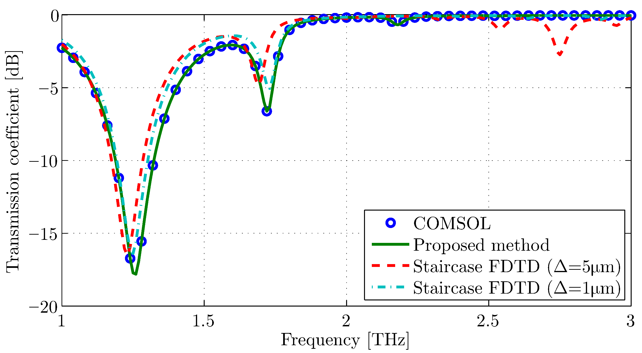
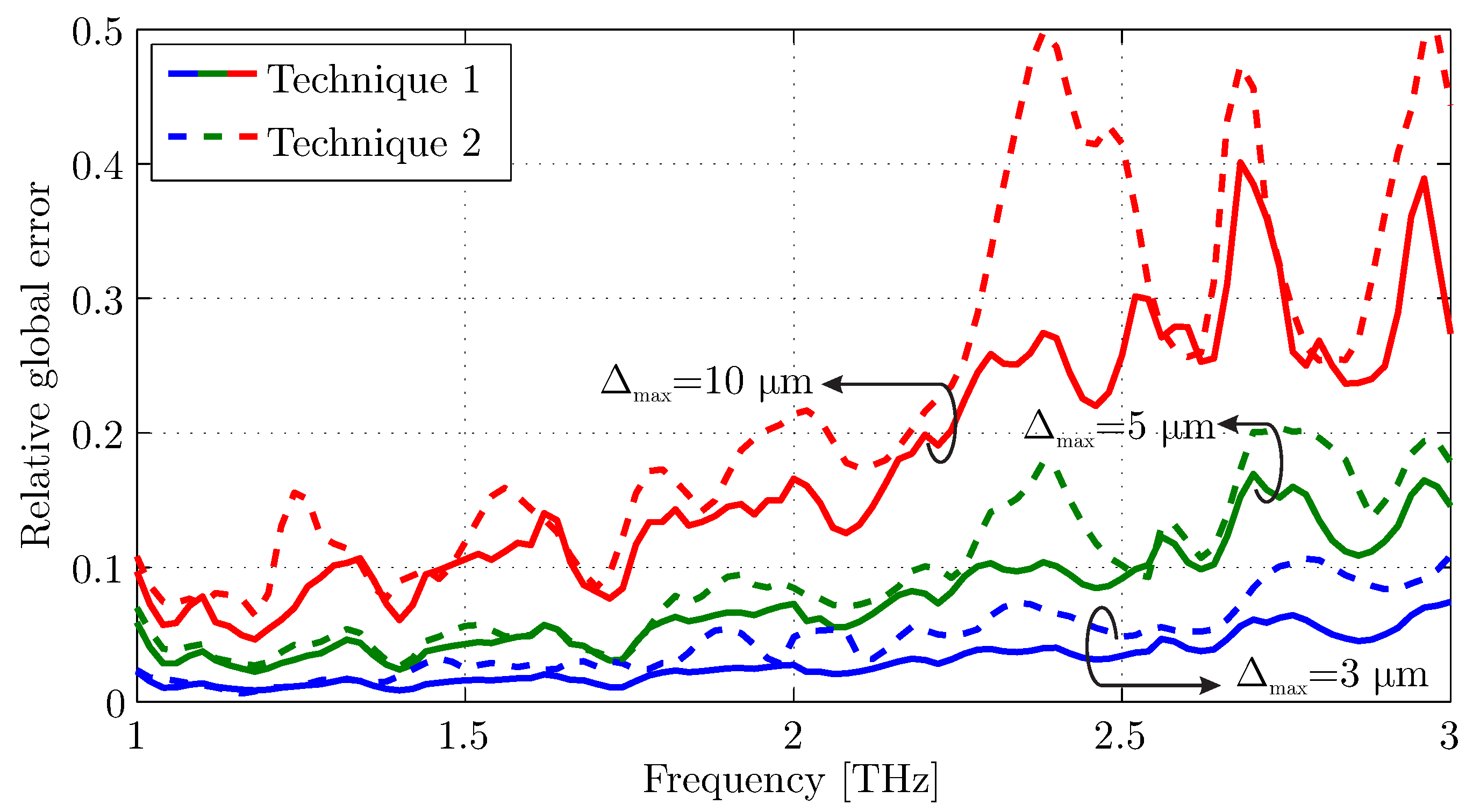
3. Proposed Algorithm Validation

The validity of the featured algorithm is pursued through the well-established setup of surface wave propagation onto a straight free-standing graphene layer of infinite size. The advantage of this example is its direct comparison to the analytical expressions (4) and (5). Moreover, the conventional FDTD method is able to provide accurate results for this orthogonal setup, in order to calculate reliably the global error within computational domain. To this aim, graphene chemical potential was selected μ c = 0.2 eV, and its scattering rate was set to Γ = 0.11 meV, while the analysis was performed at the far-infrared spectrum, namely from 1 to 3 THz. The dimension of the computational domain is 600 μ m × 150 μ m, with the graphene layer located along the x-axis. As discussed, an unstructured Delaunay triangulation was utilized with a maximum edge size Δ max = 3 μ m, resulting in approximately 32,000 elements. The time-step was selected 3.7 fs to ensure the algorithm’s stability, while open boundaries were terminated via an 8-cell thick perfectly matched layer (PML). It is important to mention that PML is selected instead of an Absorbing Boundary Condition since it is possible to extend graphene inside the PML region. This leads to the effective absorption of the strongly confined SPP waves. Finally, 8-cells are adequate for the considered applications due to the inherent losses of graphene surface waves.
The numerically extracted propagation properties of the supported surface wave on graphene are compared to the aforementioned theoretical calculations in Figure 3. It is clear that the matching of the results is evident, especially until 2.5 THz. Beyond this frequency, the SPP wavelength is less than 30 μ m, and the conventional λ / 10 discretization limit is exceeded, leading to small discrepancies. It is important to mention that the simulated results represent both magnetic-field sampling techniques, since their differences is negligible. Furthermore, the distribution of the magnetic field at 2 THz is demonstrated in Figure 4, clearly indicating the propagation of the strongly confined surface wave on the graphene surface. Consequently, the proposed integration of the infinitesimally thin material into an unstructured triangular grid was validated successfully.
Finally, the global error in the computational domain was investigated for different element sizes, to check the influence of the element size. For this reason, a numerical simulation through the conventional orthogonal grid of the FDTD method was conducted using a considerably fine mesh ( Δ x = Δ y < λ SPP / 20 ). The mean global error was calculated for the magnetic-field component, while it was normalized to the mean magnetic-field value of the computational domain. The calculated results are depicted in Figure 5, and it is apparent that smaller triangle dimensions lead to more precise results. Note that the shape of the curves is, generally, altered with Δ max since different triangular meshes are generated. In addition, the magnetic-field sampling at the triangle circumcenter (technique 1) presents a slightly lower global error. In any case, the satisfaction of the well-known Δ max < λ SPP / 10 rule secures reliable numerical results.

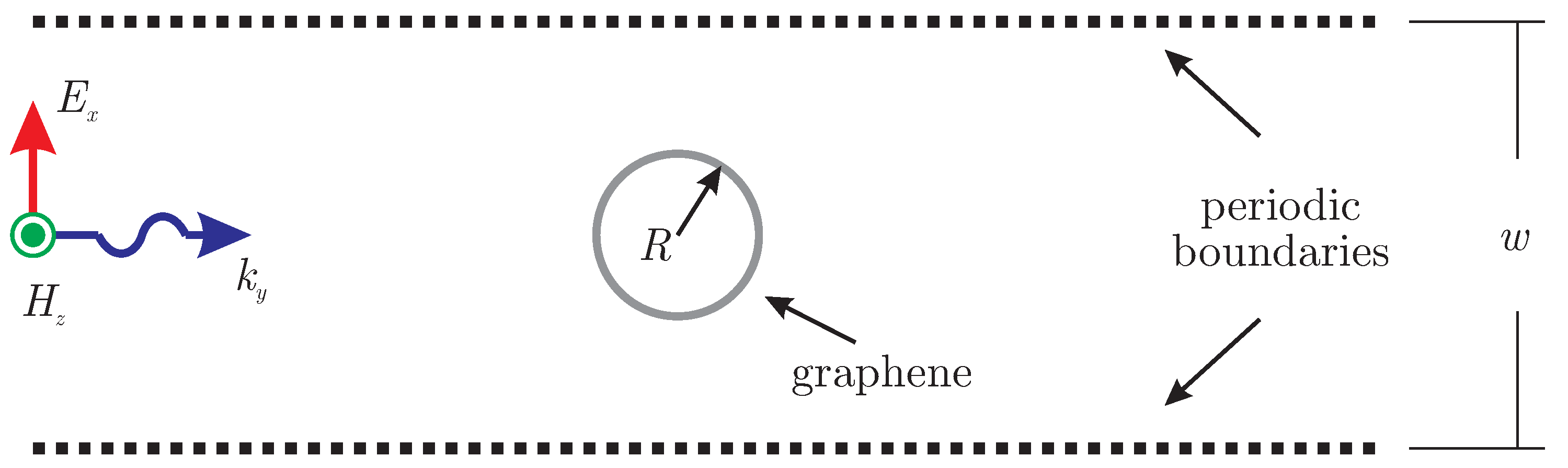
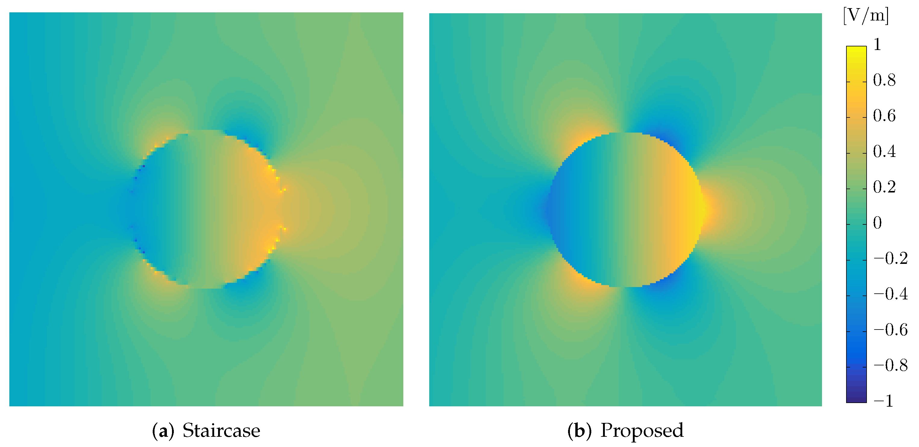
4. Incident Field toward a Circular Graphene Scatterer

Although the previous example validated the accuracy of the proposed methodology, the computational efficiency is not optimal compared to the conventional FDTD algorithm. The main reason for the degraded performance is the requirement for the storage of additional parameters, such as triangle dimensions as well as pointers to identify adjacent elements. For this reason, a second example is discussed in this section to exploit the advantages of the triangular computational domain. Particularly, a plane wave propagates toward a periodic structure of circular graphene scatterers of radius R = 20 μ m and periodicity of w = 100 μ m, as illustrated in Figure 6. The graphene chemical potential is set to 0.2 eV, and its scattering rate is 0.11 meV at the frequency range 1–3 THz. The computational domain is divided into 23,000 triangular elements of maximum edge size Δ max = 3 μ m, while the time-step is selected 3.7 fs. The side boundaries satisfy periodic conditions, and the extracted quantity of interest is the configuration’s transmission coefficient.
The extracted numerical results of the proposed algorithm are compared to the conventional staircase approximation of the FDTD algorithm, as well as the commercial software COMSOL Multiphysics® commercial package [33] for reference. Figure 7 proves the excellent behavior of our methodology. On the other hand, the staircase approximation fails to track the resonance frequencies accurately, even when using a very fine mesh ( Δ = 1 μ m). This performance is explained via the distribution of the electric field in the scatterer in Figure 8. Specifically, the edge effects of the staircase approximation degrade the plasmonic resonances on the graphene, in contrast to the proposed method, where the electric field is smoothly distributed on the material surface.

5. Conclusions

The accurate time-domain modeling of curved graphene layers was accomplished in the present work using an unstructured triangular mesh. Initially, the fundamental characteristics of the two-dimensional material were investigated, as well as the finite integration scheme for the proposed computational grid. Particularly, two techniques were examined that coincide for equilateral triangle discretization. The strength of the first one relies on its more physical representation to achieve increased accuracy, but acute triangles are required to ensure stability. This problem is resolved via the second technique, although the necessity of further approximations slightly decreases the algorithm’s accuracy. Then, graphene was introduced into the numerical algorithm as an equivalent surface current density, while its frequency dispersion was treated via an RCM technique. The proposed methodology was thoroughly examined in terms of the surface wave propagation properties, validating the proposed implementation. Finally, a circular graphene scatterer setup was designed to exploit the algorithm’s applicability and advantages, compared to the conventional staircase approximation.

Author Contributions

Conceptualization, S.A.; methodology, S.A.; validation, S.A.; writing—original draft preparation, S.A.; writing—review and editing, T.Z. and N.K.; supervision, T.Z. and N.K. All authors have read and agreed to the published version of the manuscript.

Funding

This research was cofinanced by Greece and the European Union (European Social Fund- ESF) through the Operational Programme «Human Resources Development, Education and Lifelong Learning» in the context of the project “Reinforcement of Postdoctoral Researchers—2nd Cycle” (MIS-5033021), implemented by the State Scholarships Foundation (IKY). Axioms 11 00044 i001.

Institutional Review Board Statement

Not applicable.

Informed Consent Statement

Not applicable.

Data Availability Statement

The data presented in this study are available via a straightforward reproduction of the provided simulation details.

Conflicts of Interest

The authors declare no conflict of interest.

Abbreviations

The following abbreviations are used in this manuscript:
FDTDFinite-Difference Time-Domain
PMLPerfectly Matched Layer
RCMRecursive Convolution Method
SPPSurface Plasmon Polariton

References

  1. Novoselov, K.; Geim, A.K.; Morozov, S.; Jiang, D.; Zhang, Y.; Dubonos, S.; Grigorieva, I.; Firsov, A. Electric field effect in atomically thin carbon films. Science 2004, 306, 666–669. [Google Scholar] [CrossRef] [PubMed] [Green Version]
  2. Mikhailov, S.A.; Ziegler, K. New electromagnetic mode in graphene. Phys. Rev. Lett. 2007, 99, 016803. [Google Scholar] [CrossRef] [PubMed] [Green Version]
  3. Grigorenko, A.N.; Polini, M.; Novoselov, K. Graphene plasmonics. Nat. Photonics 2012, 6, 749–758. [Google Scholar] [CrossRef]
  4. Bludov, Y.V.; Ferreira, A.; Peres, N.M.; Vasilevskiy, M.I. A primer on surface plasmon-polaritons in graphene. Int. J. Mod. Phys. B 2013, 27, 1341001. [Google Scholar] [CrossRef] [Green Version]
  5. Ansell, D.; Radko, I.; Han, Z.; Rodriguez, F.; Bozhevolnyi, S.; Grigorenko, A. Hybrid graphene plasmonic waveguide modulators. Nat. Commun. 2015, 6, 8846. [Google Scholar] [CrossRef] [PubMed]
  6. Xiao, S.; Zhu, X.; Li, B.H.; Mortensen, N.A. Graphene-plasmon polaritons: From fundamental properties to potential applications. Front. Phys. 2016, 11, 117801. [Google Scholar] [CrossRef] [Green Version]
  7. Li, Y.; Tantiwanichapan, K.; Swan, A.K.; Paiella, R. Graphene plasmonic devices for terahertz optoelectronics. Nanophotonics 2020, 9, 1901–1920. [Google Scholar] [CrossRef]
  8. Zhang, J.; Hong, Q.; Zou, J.; He, Y.; Yuan, X.; Zhu, Z.; Qin, S. Fano-resonance in hybrid metal-graphene metamaterial and its application as mid-infrared plasmonic sensor. Micromachines 2020, 11, 268. [Google Scholar] [CrossRef] [Green Version]
  9. Choroszucho, A. Analysis of the influence of the complex structure of clay hollow bricks on the values of electric field intensity by using the FDTD method. Arch. Electr. Eng. 2016, 65, 745–759. [Google Scholar] [CrossRef]
  10. Oskooi, A.F.; Roundy, D.; Ibanescu, M.; Bermel, P.; Joannopoulos, J.D.; Johnson, S.G. MEEP: A flexible free-software package for electromagnetic simulations by the FDTD method. Comput. Phys. Commun. 2010, 181, 687–702. [Google Scholar] [CrossRef]
  11. Bouzianas, G.D.; Kantartzis, N.V.; Yioultsis, T.V.; Tsiboukis, T.D. Consistent study of graphene structures through the direct incorporation of surface conductivity. IEEE Trans. Magn. 2014, 50, 161–164. [Google Scholar] [CrossRef]
  12. Ramadan, O. Improved direct integration auxiliary differential equation FDTD scheme for modeling graphene drude dispersion. Optik 2020, 219, 165173. [Google Scholar] [CrossRef]
  13. Nayyeri, V.; Soleimani, M.; Ramahi, O.M. Modeling graphene in the finite-difference time-domain method using a surface boundary condition. IEEE Trans. Antennas Propag. 2013, 61, 4176–4182. [Google Scholar] [CrossRef]
  14. Wang, X.H.; Yin, W.Y.; Chen, Z. Matrix exponential FDTD modeling of magnetized graphene sheet. IEEE Antennas Wirel. Propag. Lett. 2013, 12, 1129–1132. [Google Scholar] [CrossRef]
  15. Amanatiadis, S.A.; Kantartzis, N.V.; Ohtani, T.; Kanai, Y. Precise modeling of magnetically biased graphene through a recursive convolutional FDTD method. IEEE Trans. Magn. 2017, 54, 7201504. [Google Scholar] [CrossRef]
  16. Ramadan, O. Simplified FDTD Formulations for Magnetostatic Biased Graphene Simulations. IEEE Antennas Wirel. Propag. Lett. 2020, 19, 2290–2294. [Google Scholar] [CrossRef]
  17. Mock, A. Modeling passive mode-locking via saturable absorption in graphene using the finite-difference time-domain method. IEEE J. Quantum Electron. 2017, 53, 1300210. [Google Scholar] [CrossRef]
  18. Amanatiadis, S.A.; Ohtani, T.; Zygiridis, T.T.; Kanai, Y.; Kantartzis, N.V. Modeling the Third-Order Electrodynamic Response of Graphene via an Efficient Finite-Difference Time-Domain Scheme. IEEE Trans. Magn. 2019, 56, 6700704. [Google Scholar] [CrossRef]
  19. Mock, A. Padé approximant spectral fit for FDTD simulation of graphene in the near infrared. Opt. Mater. Express 2012, 2, 771–781. [Google Scholar] [CrossRef]
  20. Amanatiadis, S.; Zygiridis, T.; Ohtani, T.; Kanai, Y.; Kantartzis, N. A Consistent Scheme for the Precise FDTD Modeling of the Graphene Interband Contribution. IEEE Trans. Magn. 2021, 57, 1600104. [Google Scholar] [CrossRef]
  21. Xiao, S.; Wang, T.; Liu, Y.; Xu, C.; Han, X.; Yan, X. Tunable light trapping and absorption enhancement with graphene ring arrays. Phys. Chem. Chem. Phys. 2016, 18, 26661–26669. [Google Scholar] [CrossRef] [PubMed] [Green Version]
  22. Xu, H.; Zhang, Z.; Wang, S.; Liu, Y.; Zhang, J.; Chen, D.; Ouyang, J.; Yang, J. Tunable graphene-based plasmon-induced transparency based on edge mode in the mid-infrared region. Nanomaterials 2019, 9, 448. [Google Scholar] [CrossRef] [PubMed] [Green Version]
  23. Liu, T.; Zhou, C.; Jiang, X.; Cheng, L.; Xu, C.; Xiao, S. Tunable light trapping and absorption enhancement with graphene-based complementary metasurfaces. Opt. Mater. Express 2019, 9, 1469–1478. [Google Scholar] [CrossRef] [Green Version]
  24. Liu, P.; Cai, W.; Wang, L.; Zhang, X.; Xu, J. Tunable terahertz optical antennas based on graphene ring structures. Appl. Phys. Lett. 2012, 100, 153111. [Google Scholar] [CrossRef]
  25. Ye-xin, S.; Jiu-sheng, L.; Le, Z. Graphene-integrated split-ring resonator terahertz modulator. Opt. Quantum Electron. 2017, 49, 350. [Google Scholar] [CrossRef]
  26. Wu, L.; Liu, H.; Li, J.; Wang, S.; Qu, S.; Dong, L. A 130 GHz electro-optic ring modulator with double-layer graphene. Crystals 2017, 7, 65. [Google Scholar] [CrossRef] [Green Version]
  27. Bao, Z.; Tang, Y.; Hu, Z.D.; Zhang, C.; Balmakou, A.; Khakhomov, S.; Semchenko, I.; Wang, J. Inversion method characterization of graphene-based coordination absorbers incorporating periodically patterned metal ring metasurfaces. Nanomaterials 2020, 10, 1102. [Google Scholar] [CrossRef]
  28. Gusynin, V.; Sharapov, S.; Carbotte, J. Magneto-optical conductivity in graphene. J. Phys. Condens. Matter 2006, 19, 026222. [Google Scholar] [CrossRef] [Green Version]
  29. Hanson, G.W. Dyadic Green’s functions and guided surface waves for a surface conductivity model of graphene. J. Appl. Phys. 2008, 103, 064302. [Google Scholar] [CrossRef] [Green Version]
  30. Taflove, A.; Hagness, S.C.; Piket-May, M. Computational electromagnetics: The finite-difference time-domain method. In The Electrical Engineering Handbook; Elsevier Inc.: New York, NY, USA, 2005; Volume 3. [Google Scholar]
  31. Lee, C.; McCartin, B.; Shin, R.; Kong, J.A. A triangular-grid finite-difference time-domain method for electromagnetic scattering problems. J. Electromagn. Waves Appl. 1994, 8, 449–470. [Google Scholar] [CrossRef]
  32. Liu, Y.; Sarris, C.D.; Eleftheriades, G.V. Triangular-mesh-based FDTD analysis of two-dimensional plasmonic structures supporting backward waves at optical frequencies. J. Light. Technol. 2007, 25, 938–945. [Google Scholar] [CrossRef]
  33. COMSOL Multiphysics® v. 5.5, COMSOL AB. 2019. Available online: www.comsol.com (accessed on 1 November 2021).
Figure 1. Topology of the unstructured triangular grid and the electromagnetic field assignment concerning the two magnetic field sampling techniques. In particular, the arrangement of the electric components is at the edges of the triangles, while the magnetic components lie inside the triangle (a) at its circumcenter or (b) at its centroid.
Axioms 11 00044 g001
Figure 2. Block diagram of the proposed scheme.
Axioms 11 00044 g002
Figure 3. Numerical validation of surface wave propagation characteristics for a graphene layer with μ c = 0.2 eV and Γ = 0.11 meV.
Axioms 11 00044 g003
Figure 4. Distribution of the magnetic-field component for a graphene layer with μ c = 0.2 eV and Γ = 0.11 meV at 2 THz.
Axioms 11 00044 g004
Figure 5. Global error of the magnetic field, normalized to the mean computational domain value, for different triangle size discretization of the two proposed techniques.
Axioms 11 00044 g005
Figure 6. Setup of an incident plane wave toward a periodic structure of circular graphene scatterers.
Axioms 11 00044 g006
Figure 7. Transmission coefficient comparison between the proposed method and the conventional staircase FDTD algorithm for a circular graphene scatterer of 20 μ m radius.
Axioms 11 00044 g007
Figure 8. Comparison of the electric field distribution between the proposed method and the conventional staircase FDTD algorithm for a circular graphene scatterer of 20 μ m radius at 1.72 THz.
Axioms 11 00044 g008
Publisher’s Note: MDPI stays neutral with regard to jurisdictional claims in published maps and institutional affiliations.

