Article

Fractional Clique Collocation Technique for Numerical Simulations of Fractional-Order Brusselator Chemical Model

by
Mohammad Izadi
1 and
Hari Mohan Srivastava
2,3,4,5,*
1
Department of Applied Mathematics, Faculty of Mathematics and Computer, Shahid Bahonar University of Kerman, Kerman 76169-14111, Iran
2
Department of Mathematics and Statistics, University of Victoria, Victoria, BC V8W 3R4, Canada
3
Department of Medical Research, China Medical University Hospital, China Medical University, Taichung 40402, Taiwan
4
Department of Mathematics and Informatics, Azerbaijan University, 71 Jeyhun Hajibeyli Street, AZ1007 Baku, Azerbaijan
5
Center for Converging Humanities, Kyung Hee University, 26 Kyungheedae-ro, Dongdaemun-gu, Seoul 02447, Republic of Korea
*
Author to whom correspondence should be addressed.
Axioms 2022, 11(11), 654; https://doi.org/10.3390/axioms11110654
Submission received: 14 October 2022 / Revised: 14 November 2022 / Accepted: 16 November 2022 / Published: 18 November 2022
(This article belongs to the Special Issue Theory of Functions and Applications)

Abstract

:
The primary focus of this research study is in the development of an effective hybrid matrix method to solve a class of nonlinear systems of equations of fractional order arising in the modeling of autocatalytic chemical reaction problems. The fractional operator is considered in the sense of Liouville–Caputo. The proposed approach relies on the combination of the quasi-linearization technique and the spectral collocation strategy based on generalized clique bases. The main feature of the hybrid approach is that it converts the governing nonlinear fractional-order systems into a linear algebraic system of equations, which is solved in each iteration. In a weighted L 2 norm, we prove the error and convergence analysis of the proposed algorithm. By using various model parameters in the numerical examples, we show the computational efficacy as well as the accuracy of our approach. Comparisons with existing available schemes show the high accuracy and robustness of the designed hybrid matrix collocation technique.

1. Introduction

The Brusselator is a theoretical model for a type of autocatalytic reaction. In fact, this model is a common nonlinear reaction in which a reactant species interacts with other species to increase its production rate. The Brusselator model was proposed by Prigogine and Lefever [1] in 1968. It is also known that the Belousov–Zhabotinsky model and the chemical reactions of the Brusselator are the same [2,3,4]. By U , V , D , A , B , and E, we denote the chemical components in the chemical reaction. Generally, the reaction process can be described by the following four steps:
  • A U ,
  • B + U V + D ,
  • 2 U + V 3 U ,
  • U E .
We now assume that the species A and B are sufficiently available and can thus be modeled at a constant concentration. Further, note that the final products E and D are removed once they are produced from the reaction process. Under scaling the rate constant to unity, the rate equations become as follows
d d t { U } = { A } + { U } 2 { V } { B } { U } { U } , d d t { V } = { B } { U } { U } 2 { V } .
Fractional integrals and derivatives have attracted considerable attention over the last decades. Due to a wide range of applications from theory to practice, they have gained increasing popularity in the modeling of various natural phenomena in engineering, physics, chemistry, economics, etc. It is found that the non-integer derivatives and integrals are more appropriate for describing the properties of several real processes and materials, see cf. [5,6]. However, the solutions to most fractional differential equations do not exist in terms of elementary functions. Therefore, it is essential to develop computational and approximate procedures for the numerical evaluation of fractional differential equations.
Our main goal is to study the fractional counterpart of the Brusselator model (1). To be precise, this research paper presents a power series solution based upon the (fractional) version of clique functions implemented in matrix formulation for the following nonlinear fractional-order Brusselator system of two equations
LC D τ λ u ( τ ) = θ ( η + 1 ) u ( τ ) + u 2 ( τ ) v ( τ ) , LC D τ λ v ( τ ) = η u ( τ ) u 2 ( τ ) v ( τ ) , τ [ 0 , 1 ] ,
where θ and η are two positive real numbers. Moreover, LC D τ λ presents the Liouville–Caputo fractional derivative of order λ ( 0 , 1 ] . The following initial conditions will accompany the above system, given as
u ( 0 ) = u 0 , v ( 0 ) = v 0 .
If we set λ = 1 , the classical system of the Brusselator system (1) will be obtained. The integer-order model of the Brusselator has been solved by three numerical approaches, including the Implicit Runge–Kutta method, the Adams method, and the Backward differential formula in [7].

1.1. Literature Review and Related Works

The fractional-order system (2) has been considered in the literature by many research scholars from different points of dynamic systems and numerical behaviors. The stability of the fractional Brusselator system was addressed in [8,9,10]. In [11], the existence of a limit cycle was proven numerically by the Adams–Bashforth–Moulton approach. The authors of [12,13] developed some nonstandard finite difference (NSFD) methods to solve (2) numerically. As a semi-analytical approach, the variational iteration method is devised in [14]. The polynomial least square technique was investigated in [15]. The operational matrix methods based on Bernstein and Legendre wavelet functions were studied in [16,17], respectively. The authors of [18] further developed three explicit and implicit techniques based on product integration, NFSD, and multi-step procedures. In all mentioned works above, the underlying fractional operator was taken as the Liouville–Caputo fractional derivative. However, let us mention that the Brusselator model with fractional derivatives in the sense of Liouville–Caputo, Caputo–Fabrizio, and Atangana–Baleanu was considered in [19] recently. In this paper, the dynamic characteristics of the model under three fractional derivatives have been investigated, and a three-stage iterative approach was also developed for the model under consideration. In addition, in [20], the fractal-fractional differential operators related to the power law, exponential decay, and the generalized Mittag–Leffler kernels were investigated. In the latter research work, the proposed numerical procedure is based on the Lagrange interpolating polynomial together with the theory of fractional calculus. Finally, let us mention that the PDE counterpart of the Brusselator model (2) has been investigated in the literature. Among others, we refer to the published papers [21,22,23,24]

1.2. Outline of This Paper

The primary purpose of the current research paper is to propose an effective hybrid technique. Our novel method is based on a combination of the quasi-linearization approach and matrix collocation method for an approximate treatment of the fractional Brusselator equations. The idea of a quasi-linearization method (QLM) is used to convert the nonlinear model into a family of linearized equations. Afterward, the spectral approach based on the (novel) generalized clique functions (GCFs) is employed to solve the quasi-linear equations in an iterative manner. Let us emphasize that the coefficients of all clique polynomials are all positive and integer-compared to the classical set of polynomials, such as Legendre, Chebyshev, Hermit, Laguerre, etc. Consequently, working with positive numbers yields more stable results during the computations. This would be the main motivation to employ the family of clique polynomials in the collocation matrix procedure over others. Another major advantage of the presented hybrid method, namely QLM-GCFs, is that it is not only effective in terms of required CPU time, but it provides high-order accuracy and better resolution characteristics compared to the existing numerical models in the literature. The accurateness and robustness of the spectral collocation strategies have been justified successfully by applying various model equations. Among others, let us mention the works [25,26,27,28,29,30].
The content of this research paper is organized as follows. Some basic facts on fractional calculus are reviewed in Section 2. Section 3 is devoted to the definition of clique basis functions. Moreover, a generalization of these functions is given. Then, the convergence analysis of this basis function is established in a weighted L 2 norm. A detailed description of the present QLM-GCFs technique is provided in Section 4. The results of the performed numerical simulations and experiments are given in Section 5. The concluding summary is given in Section 6.

2. Fractional Calculus: Basic Facts

Let us give some important facts about fractional calculus that will be used in the subsequent sections. For more detail, we refer the readers to the standard text [6] or some recent expository papers [31,32].
Let us first recall that the Riemann–Liouville fractional integral operator of order λ > 0 is given by
0 I τ λ [ k ] ( τ ) = 1 Γ ( λ ) 0 τ k ( r ) ( τ r ) 1 λ d r ,
where Γ ( · ) is the Gamma function and we assumed k ( τ ) C ξ , ξ > 1 . We note that a real function k ( τ ) , τ > 0 belongs to the space C ξ , ξ R if there exists a number μ R and a function l ( τ ) C ( [ 0 , ) such that k ( τ ) = τ μ l ( τ ) . We also call that k ( τ ) C ξ n if and only if k ( n ) ( τ ) C ξ for a n N .
We are now ready to define the fractional Liouville–Caputo derivative next.
Definition 1.
Assume that k C 1 n and n 1 < λ < n , n N . The Liouville–Caputo fractional derivative of k ( τ ) of order λ is defined by
LC D τ λ k ( τ ) = 0 I τ n λ [ D n k ] ( τ ) = 1 Γ ( n λ ) 0 τ ( τ r ) n λ 1 k ( n ) ( r ) d r , τ > 0 ,
where D = d d τ .
One should emphasize that the fractional operator LC D τ λ is a linear operator. If C is a constant number, we have
LC D τ λ C = 0 .
Our next goal is to compute the Liouville–Caputo fractional derivative of the function k ( τ ) = τ p , where p is a constant. This can be performed through the following relations
LC D τ λ τ p = 0 , for κ N 0 and p < λ , Γ ( p + 1 ) Γ ( p + 1 λ ) τ p λ , for p N 0 and p λ or p N and p > λ .
Note that N 0 : = N { 0 } and also we have utilized · and · as the ceil and floor functions respectively.

3. The Fractional-Order Clique Polynomial and Its Convergence Analysis

Here, we first consider the clique polynomials C r ( t ) related to the cliques in a complete graph. We then introduce the fractional version of these polynomials. Hence, we establish the convergence analysis of these polynomials.

3.1. The Clique Functions: The Generalized Form

The clique polynomials were first introduced in [33] and associated with graph theory. However, they have been recently considered for numerical approximations of ordinary and fractional differential equations, see cf. [34,35,36,37]. Below, we first describe the main aspects of them.
Definition 2.
Over a bounded interval of the real line [ a , b ] , ( b > a 0 ), we define the clique functions (CFs) as follows:
C r ( t ) : = k = 0 r r k t k .
For r = 0 , 1 in (6), we get C 0 ( t ) = 1 and C 1 ( t ) = 1 + t . One can easily observe that the following recursive formulation holds for this set of polynomials
C r + 1 ( t ) = ( 1 + t ) C r ( t ) , r = 0 , 1 , , C 0 ( t ) = 1 .
By using recursion (7), we derive a few terms of CFs as
C 2 ( t ) = t 2 + 2 t + 1 , C 3 ( t ) = t 3 + 3 t 2 + 3 t + 1 , C 4 ( t ) = t 4 + 4 t 3 + 6 t 2 + 4 t + 1 .
One can easily check that C r ( 0 ) = 1 and C r ( 1 ) = 2 r for all values of r 0 . It is not a difficult task to check that these CFs satisfy a second-order differential equation in the form
d d t ( t + 1 ) 2 d d t C r ( t ) = r ( r + 1 ) C r ( t ) , r N 0 .
In what follows, we intend to use the CFs on an arbitrary interval D a , b : = [ a , b ] . We are also interested in using the generalized version of these polynomials of fractional order 0 < α 1 .
Definition 3.
Generalized CFs (GCFs) of degree r on D a , b are represented by C r α ( τ ) and defined by
C r α ( τ ) = C r ( t ) , t = τ L α ,
where L = b a .
With the help of this transformation, the explicit form in (6) will be given as follows:
C r α ( τ ) = k = 0 r 1 L k α r k τ k α , r N .

3.2. L 2 -Convergent of GCFs

Let us investigate the convergence analysis of the GCFs in a weighted L 2 norm. In other words, we will investigate the behavior of the expansion series of a given function with respect to GCFs, especially when we increase the number of bases. We associate the following space to domain D a , b as [25]
L 2 , w ( D a , b ) = { : D a , b R | is   measurable   and w < } , w ( τ ) = 1 / L ,
Here, the related induced norm and inner product are given by
( τ ) , k ( τ ) w = a b ( τ ) k ( τ ) w ( τ ) d τ , w 2 = a b | ( τ ) | 2 w ( τ ) d τ
Practically, a finite-dimensional subset, say S R , of the space L 2 , w ( D a , b ) is selected as
S R = span C 0 α ( τ ) , C 1 α ( τ ) , , C R α ( τ ) .
One observes that dim ( S R ) = R + 1 and is also a closed subspace of L 2 , w ( D a , b ) . It follows that S R is a complete subspace of L 2 , w ( D a , b ) . Thus, any given function L 2 , w ( D a , b ) has a unique best (finest) approximation S R in the following sense that
( τ ) ( τ ) w ( τ ) h ( τ ) ω , h S R .
Generally, a given function ( τ ) L 2 , w ( D a , b ) can be expressed as a linear combination of GCFs. Thus, we have
( τ ) = r = 0 κ r C r α ( τ ) , τ D a , b .
Here, the coefficients of κ r are unknown for r = 0 , 1 , . By truncating the former series up to ( R + 1 ) terms, we may approximate ( τ ) in practice as
( τ ) R ( τ ) = r = 0 R κ r C r α ( τ ) = C R α ( τ ) K R ,
where we have represented the involved finite series in a compact way by defining
C R α ( τ ) = C 0 α ( τ ) C 1 α ( τ ) C R α ( τ ) , K R = κ 0 κ 1 κ R T .
Note that the first one is the vector of GCFs while K R is the vector of unknowns. To derive an upper bound for the E R ( τ ) = ( τ ) R ( τ ) , we need the following result. A proof of the next theorem can be found in [38].
Theorem 1.
Let C R ( D a , b ) . If l R ( τ ) represents the interpolating function of ℓ at R Chebyshev points on D a , b , then we have
| ( τ ) l R ( τ ) | 2 L R R , 4 R R ! , R , : = max τ D a , b | ( R ) ( τ ) | .
Following [39], we establish the following error bound for the GCFs expansion series.
Theorem 2.
Suppose that C R ( D a , b ) L w , 2 ( D a , b ) . If R ( τ ) = C R α ( τ ) K R presents the best (finest) approximation of ( τ ) out of S R , α , then an error bound is given by
E R w 2 R , 4 R R ! .
Proof. 
Let us first define the new function z ( t ) : = ( t 1 α ) on D a , b α : = [ a α , b α ] and for any α > 0 . Applying Theorem 1 to function z ( t ) with R Chebyshev nodes leads to the following error estimate
| z ( t ) l R ( t ) | 2 z R , 4 R R ! , t D a , b α .
We next substitute t = τ α in the preceding inequality. It follows that
| ( τ ) l R ( τ α ) | 2 R , 4 R R ! , τ D a , b .
According to the theorem’s assumption, we know that the approximate solution R ( τ ) is the finest approximation belonging to the space S R , α . Thus, it holds that
( τ ) R ( τ ) w ( τ ) h ( τ ) w , h S R .
The former inequality is valid, particularly for h = l R ( τ α ) S R , α . Employing this fact, as well as (15), we conclude that
( τ ) R ( τ ) w 2 ( τ ) l R ( τ α ) w 2 = a b | ( τ ) l R ( τ α ) | 2 w ( τ ) d τ a b 2 R , 4 R R ! 2 w ( τ ) d τ 2 R , 4 R R ! 2 a b w ( τ ) d τ .
Using the fact that a b w ( τ ) d τ = 1 , we only require the application of the square roots to the foregoing inequality.    □

4. The Methodology of the QLM-GCFs Scheme

Instead of applying the direct collocation procedure to the underlying nonlinear model (2), our main aim is first to employ the quasi-linearization method (QLM) for (2) with initial conditions (3). Then, the generalized CFs (GCFs) collocation matrix technique is applied to the resultant family of linear subequations in an iterative manner.

4.1. The Basic Concept of QLM

By employing QLM, we can overcome the nonlinearity of a given model equation. The applicability of the QLM strategy has already been checked through tremendous research studies in the literature. For recent applications, we refer readers to [40,41,42,43].
By rewriting first the nonlinear coupled system (2) in a matrix representation form, we get
Z ( λ ) ( τ ) = F ( Z ( τ ) , τ ) .
Here, we have utilized the following notations
Z ( τ ) : = u ( τ ) v ( τ ) , Z ( λ ) ( τ ) : = LC D τ λ u ( τ ) v ( τ ) , F ( Z ( τ ) , τ ) : = θ ( η + 1 ) u ( τ ) + u 2 ( τ ) v ( τ ) η u ( τ ) u 2 ( τ ) v ( τ ) .
Suppose that Z 0 ( τ ) is a rough first approximation of Z ( τ ) . Thus, the QLM for (17) is written for p = 0 , 1 , as
Z p + 1 ( λ ) ( τ ) F ( Z p ( τ ) , τ ) + F Z ( Z p ( τ ) , τ ) Z p + 1 ( τ ) Z p ( τ ) .
Here, by F Z = d d Z F , we denote the corresponding Jacobian matrix. Let us note that the same initial conditions as (3) will be given to the last sequence of equations. After performing some straightforward calculations, we receive the following family of a linear system of equations as the result of QLM from model (17). Thus, we have
LC D τ λ Z p + 1 ( τ ) + ξ p ( τ ) Z p + 1 ( τ ) = s p ( τ ) , p = 0 , 1 , ,
where
Z p + 1 ( τ ) = u p + 1 ( τ ) v p + 1 ( τ ) , ξ p ( τ ) = η + 1 2 u p ( τ ) v p ( τ ) u p 2 ( τ ) η + 2 u p ( τ ) v p ( τ ) u p 2 ( τ ) , s p ( τ ) = θ 2 u p 2 ( τ ) v p ( τ ) 2 u p 2 ( τ ) v p ( τ ) .
Systemically, we can present the initial conditions (3) as
Z p + 1 ( 0 ) = u p + 1 ( 0 ) v p + 1 ( 0 ) = u 0 v 0 .
To solve the quasi-linear systems (18)–(19) accurately, we will design a matrix collocation procedure based on the GCFs to receive an approximate solution.

4.2. The QLM-GCFs Technique

Supposedly, the unknown solutions of quasi-linear model (18) can be expanded as a combination of the cut series form (13) with ( R + 1 )-terms. Further, assume that for a fixed α ( 0 , 1 ] the approximate solutions U R , α ( p ) ( τ ) and V R , α ( p ) ( τ ) to u p ( τ ) and v p ( τ ) in the iteration p for p = 0 , 1 , are known. For p = 0 , we utilize the initial guess Z 0 ( τ ) as the starting point. In the next iteration, p + 1 , we seek the approximate solutions in the forms
u p + 1 ( τ ) U R , α ( p + 1 ) ( τ ) = r = 0 R κ r , 1 ( p ) C r α ( τ ) , v p + 1 ( τ ) V R , α ( p + 1 ) ( τ ) = r = 0 R κ r , 2 ( p ) C r α ( τ ) ,
for τ D a , b . Below, our primary job is to find the unknown coefficients { κ r , j ( p ) } r = 0 R for j = 1 , 2 and p = 1 , 2 , by using a spectral matrix collocation approach relying on the GCFs. To this end, we first construct the matrix forms of the approximate solutions given in 20. Similar to (13), the finite series solutions in ((20)) for j = 1 , 2 can be expressed as
r = 0 R κ r , j ( p ) C r α ( τ ) = C R α ( τ ) K R , j ( p ) ,
where the unknown vectors K R , j ( p ) and the vector of GCFs are given by
K R , j ( p ) = κ 0 , j ( p ) κ 1 , j ( p ) κ R , j ( p ) T , C R α ( τ ) = C 0 α ( τ ) C 1 α ( τ ) C R α ( τ ) .
In the next Lemma, we further write the vector of basis functions in terms of monomials multiplied by a constant matrix.
Lemma 1.
The representation of the vector of GCFs is given by
C R α ( τ ) = Π R α ( τ ) M R ,
where Π R α ( τ ) = 1 τ α τ 2 α τ R α and M R of size ( R + 1 ) × ( R + 1 ) is an upper triangular matrix whose components are obtained via (10). It reads
M R = 0 0 1 0 2 0 R 1 0 R 0 0 μ 1 1 1 μ 1 2 1 μ 1 R 1 1 μ 1 R 1 0 0 μ 2 2 2 μ 2 R 1 2 μ 2 R 2 0 μ R 1 R 1 R 1 μ R 1 R R 1 0 μ R R R , μ j : = L j α , j = 1 , 2 , , R .
Proof. 
By virtue of relation (10), it is sufficient to multiply matrix M R by Π R α ( τ ) from the left.    □
Obviously, the diagonal elements of matrix M R are all non-zero. Thus, this matrix is non-singular. In fact, we have det ( M R ) = L R α ( R + 1 ) / 2 .
If one combines two former relations (21) and (22), the approximate solutions are written as
U R , α ( p + 1 ) ( τ ) = C R α ( τ ) K R , 1 ( p ) = Π R α ( τ ) M R K R , 1 ( p ) , V R , α ( p + 1 ) ( τ ) = C R α ( τ ) K R , 2 ( p ) = Π R α ( τ ) M R K R , 2 ( p ) , τ D a , b .
Next, we need the λ -derivative of the approximate solutions. To do so, we apply the operator LC D τ λ to both sides of the relation (23). Thus, we get
LC D τ λ U R , α ( p + 1 ) ( τ ) = LC D τ λ Π R α ( τ ) M R K R , 1 ( p ) , LC D τ λ V R , α ( p + 1 ) ( τ ) = LC D τ λ Π R α ( τ ) M R K R , 2 ( p ) .
Consequently, we must only compute the λ -derivatives of the vector Π R α ( τ ) . In this respect, we consider two properties (4) and (5) to calculate the fractional derivatives of Π R α ( τ ) . As an example, we set R = 3 and λ = 3 4 . Now, using α = 1 and α = 1 2 we get, respectively,
LC D τ 3 4 Π 5 1 ( τ ) = 0 1 ! Γ ( 5 4 ) τ 1 4 2 ! Γ ( 9 4 ) τ 5 4 3 ! Γ ( 13 4 ) τ 9 4 , LC D τ 3 4 Π 5 1 2 ( τ ) = 0 0 1 ! Γ ( 5 4 ) τ 1 4 Γ ( 5 2 ) Γ ( 7 4 ) τ 3 4 .
Practically, however, we can use the modified version of Algorithm 4.1 in [44] or [45] or Algorithm 3.1 in [46] with linear complexity O ( R + 1 ) to compute the λ -derivative of Π R α ( τ ) . To continue, let us define the fractional derivative of the vector as
Π R ( λ , α ) ( τ ) : = LC D τ λ Π R α ( τ ) .
We can now place this relation into (24) to arrive at
LC D τ λ U R , α ( p + 1 ) ( τ ) = Π R ( λ , α ) ( τ ) M R K R , 1 ( p ) , LC D τ λ V R , α ( p + 1 ) ( τ ) = Π R ( λ , α ) ( τ ) M R K R , 2 ( p ) .
We come back to the matrix differential Equation (18). Vector Z p + 1 ( τ ) and its derivative LC D τ λ Z p + 1 ( τ ) can be approximated as
Z p + 1 Z R ( p + 1 ) ( τ ) : = U R , α ( p + 1 ) ( τ ) V R , α ( p + 1 ) ( τ ) , LC D τ λ Z p + 1 ( τ ) LC D τ λ Z R ( p + 1 ) ( τ ) : = LC D τ λ U R , α ( p + 1 ) ( τ ) LC D τ λ V R , α ( p + 1 ) ( τ ) .
Lemma 2.
In the matrix formats, the approximated solution Z R ( p + 1 ) ( τ ) , and its λ-derivative LC D τ λ Z R ( p + 1 ) ( τ ) in (27) can be stated as follows:
Z R ( p + 1 ) ( τ ) = Π ^ ( τ ) M ^ K ^ ( p ) , LC D τ α Z R ( p + 1 ) ( τ ) = Π ^ λ ( τ ) M ^ K ^ ( p ) ,
where the following notations are used: K ^ ( p ) = K R , 1 ( p ) K R , 2 ( p ) T and
Π ^ ( τ ) = Π R α ( τ ) 0 0 Π R α ( τ ) , M ^ = M R 0 0 M R , Π ^ λ ( τ ) = Π R ( λ , α ) ( τ ) 0 0 Π R ( λ , α ) ( τ ) .
Proof. 
To conclude the results, we need to substitute two relations (23) and (26) into the corresponding vector forms in (27).    □
We are then looking for a partitioning D a , b that will be used as a set of collocation points. To do so, we utilize ( R + 1 ) equidistant points from interval [ a , b ] . Let us set
τ ρ : = a + L R ρ , ρ = 0 , 1 , , R .
Now, adding the aforementioned set of collocation points into the sequence of linear matrix differential equations (18) to get
LC D τ λ Z p + 1 ( τ ρ ) + ξ p ( τ ρ ) Z p + 1 ( τ ρ ) = s p ( τ ρ ) , ρ = 0 , 1 , , R ,
for p = 0 , 1 , . We next introduce the following matrix and vector notations
Σ p λ = LC D τ λ Z p + 1 ( τ 0 ) LC D τ λ Z p + 1 ( τ 1 ) LC D τ λ Z p + 1 ( τ R ) , Σ p = Z p + 1 ( τ 0 ) Z p + 1 ( τ 1 ) Z p + 1 ( τ R ) , S p = s p ( τ 0 ) s p ( τ 1 ) s p ( τ R ) , Ξ p = ξ p ( τ 0 ) 0 0 0 ξ p ( τ 1 ) 0 0 0 ξ p ( τ R ) .
In the vector representation, we are able to show relation (30) in a compact formulation as
Σ p λ + Ξ p Σ p = S p , p = 0 , 1 , .
Our next aim is to derive the matrix expressions of Σ p and Σ p λ . By collocating two relations (28) at the collocations points, we render
Lemma 3.
The two relations (28) at the collocation point (29) can be written as follows:
Σ p = Π ^ ˜ M ^ K ^ ( p ) , Σ p λ = Π ^ ˜ λ M ^ K ^ ( p ) ,
where the two matrices Π ^ ˜ and Π ^ ˜ λ are given by
Π ^ ˜ = [ Π ^ ( τ 0 ) Π ^ ( τ 1 ) Π ^ ( τ R ) ] T , Π ^ ˜ λ = [ Π ^ λ ( τ 0 ) Π ^ λ ( τ 1 ) Π ^ λ ( τ R ) ] T .
Here, the three matrices M ^ , Π ^ , and Π ^ λ , as well as the vector K ^ ( p ) , are defined in (28) previously.
Finally, we form the so-called fundamental matrix equation at each iteration p by placing the preceding relations (32) into (31). It follows that
A p K ^ ( p ) = S p , o r A p ; S p , p = 0 , 1 , ,
where
A p : = Π ^ ˜ λ + Ξ p Π ^ ˜ M ^ .
It should be noted that the last matrix equation (33) is a linear system with 2 ( R + 1 ) unknowns κ r , j ( p ) for r = 0 , 1 , , R and j = 1 , 2 to be specified as the coefficients of GCFs in the series solutions (20). However, the supplemented initial conditions (3) are not yet implemented and entered into the system (33). First, we consider the matrix representation forms (28) for the approximate solution Z R ( p + 1 ) ( τ ) . We then let τ 0 arrive at
A 0 , p ^ K ^ ( p ) = S ^ 0 , A 0 , p ^ : = Π ^ ( 0 ) M ^ , S ^ 0 = u 0 v 0 , o r A 0 , p ^ ; S ^ 0 .
Here, the two constants u 0 and v 0 , are available from (3). The replacement of two rows of the matrix [ A p ; S p ] in (33) will be carried out next by the row matrix A 0 , p ^ ; S ^ 0 . The modified fundamental matrix equation will be shown by
A p ^ K ^ ( p ) = S p ^ , o r A p ^ ; S p ^ .
To get the unknown coefficients of GCFs, it is sufficient to solve the modified algebraic linear system (34) in each iteration. Now, one requires a linear solver to be used to receive the solution of this system. After finding vector K ^ ( p ) , all unknowns κ r , j ( p ) , for j = 1 , 2 , and r = 0 , 1 , , R as the coefficients in the expansion series (20) will be found in iteration p. Thus, we get an approximate solution of model (2).
Algorithmically, we summarize all of the steps of the proposed QLM-GCs technique in Algorithm 1. Here, by p max we denote the maximum number of iterations required to achieve the desired accuracy in the QLM method. It should be remarked that we have utilized the MATLAB notation A [ i : j , s : k ] to denote the submatrix of A formed by all entries in the intersection of rows i , , j and columns s , , k .
Algorithm 1: An algorithmic description of the QLM-GCFs.
  1: procedure QLM_GCFs ( R , λ , α , θ , η , M R , C R α ( τ ) , u 0 , v 0 , p max )
  2: p : = 0 ;    m : = R + 1 ;     n : = 2 ;
  3: Π R α ( τ ) : = 1 τ α τ 2 α τ R α ;
  4: Π R ( λ , α ) ( τ ) : = LC D τ λ Π R α ( τ ) ;{Via calling to Algorithm 4.1 from [44]}
  5: Π ^ ( τ ) : = Π R α ( τ ) 0 0 Π R α ( τ ) ; M ^ : = M R 0 0 M R ; Π ^ λ ( τ ) = Π R ( λ , α ) ( τ ) 0 0 Π R ( λ , α ) ( τ ) ;
  6: Z p ( τ ) : = 0 ;    u p ( τ ) : = Z p [ 1 ] ;    v p ( τ ) : = Z p [ 2 ] ;
  7: ξ p ( τ ) : = η + 1 2 u p ( τ ) v p ( τ ) u p 2 ( τ ) η + 2 u p ( τ ) v p ( τ ) u p 2 ( τ ) ; s p ( τ ) : = θ 2 u p 2 ( τ ) v p ( τ ) 2 u p 2 ( τ ) v p ( τ ) ;
  {Using the collocation points (29)}
  8:  Ξ p : = 0 ;    S p : = 0 ;    Ξ p R n m × n m  &  S p R n m × 1
  9:  Π ^ ˜ : = 0 ;    Π ^ ˜ λ = 0 ;    Π ^ ˜ , Π ^ ˜ λ R n m × n m
  10: for j : = 0 , , R
  11:   Ξ p [ n j + 1 : n ( j + 1 ) , n j + 1 : n ( j + 1 ) ] : = ξ p ( τ j ) ;
  12:    S p [ n j + 1 : n ( j + 1 ) ] : = s p ( τ j ) ;
  13:   Π ^ ˜ [ n j + 1 : n ( j + 1 ) , n j + 1 : n ( j + 1 ) , : ] : = Π ^ ( τ j ) ;
  14:    Π ^ ˜ λ [ n j + 1 : n ( j + 1 ) , n j + 1 : n ( j + 1 ) , : ] : = Π ^ ( τ j ) ;
  15:end for
  16:for  p : = 1 , , p max
  17:  Fa_Sys:= Π ^ ˜ λ + Ξ p Π ^ ˜ λ M ^ ;   rhs_Sys:= S p ;
  {Entering the I.C.}
  18:  Fa_Sys[1:2,:]:= Π ^ ( 0 ) M ^ ;    rhs_Sys[1:2]:= [ u 0 , v 0 ] T ;
  19:   K ^ ( p ) :=LinSolve (Fa_Sys,rhs_Sys);
  20:   U R , α ( p ) ( τ ) : = C R α ( τ ) K R , 1 ( p ) ;    V R , α ( p ) ( τ ) : = C R α ( τ ) K R , 2 ( p ) ;
  21:  Update ξ p ( τ ) and s p ( τ ) in line 7 in terms of the former solutions;
  22:  Calculate two matrices Ξ p and S p in lines 11-12;
  23: end for
  24: end;

5. Numerical Results and Graphical Representations

In this part, a set of computational examples is provided to describe and support the theoretical findings. In this respect, we apply the QLM-GCFs to the fractional-order Brusselator of Equation (2) by solving the quasi-linear model Equation (17). For performing computational simulations, we use Matlab software version 2021a on a computer with 16 GB of RAM and a CPU with 2.2 GHz Intel® Core™ i7-10870H processor.
In the computational results, we utilize the QLM with parameter p = 5 . Furthermore, in the QLM-GCFs, the initial approximation Z 0 ( τ ) is selected as the zero function, or we take it as the initial condition (3). As previously mentioned, the exact solutions of this system are not available, especially when the order of the derivative is described in the fractional order. Therefore, we define the residual error functions (REFs) associated with the Brusselator model to measure the accuracy of the proposed spectral QLM-GCFs collocation technique. That is, in iteration p = 1 , 2 , , we define the error terms as
Res u , R , α ( p ) ( τ ) : = LC D τ λ U R , α ( p ) ( τ ) θ + ( η + 1 ) U R , α ( p ) ( τ ) U R , α ( p ) ( τ ) 2 V R , α ( p ) ( τ ) 0 , Res v , R , α ( p ) ( τ ) : = LC D τ λ V R , α ( p ) ( τ ) η U R , α ( p ) ( τ ) + U R , α ( p ) ( τ ) 2 V R , α ( p ) ( τ ) 0 .
We also compute the L error norms (for a fixed p) via the relations
L u L u ( R ) : = max τ D a , b Res u , R , α ( p ) ( τ ) , L v L v ( R ) : = max τ D a , b Res v , R , α ( p ) ( τ ) .
We further utilize the following relations to compute the obtained numerical order of convergence (Noc) related to the numerical technique applied to both solutions of the coupled system (2) given by
Noc u : = log 2 L u ( R ) L u ( 2 R ) , Noc v : = log 2 L v ( R ) L v ( 2 R ) .
Note that these formulae are utilized to check the order of accuracy of our proposed technique in the L norm for both solutions.
Example 1.
As the first test case, let us consider the fractional Brusselator system by taking two parameters θ = 0 and η = 1 to get
LC D τ λ u ( τ ) = 2 u ( τ ) + u 2 ( τ ) v ( τ ) , LC D τ λ v ( τ ) = u ( τ ) u 2 ( τ ) v ( τ ) , λ ( 0 , 1 ] .
The given initial conditions are u ( 0 ) = 1 , v ( 0 ) = 1 . This example was considered in [14,16,17] previously.
Let us first set a = 0 , b = 1 and take R = 5 . We also consider λ = 1 . Using α = 1 , the proposed QLM-GCFs with the collocation points { 0 , 2 / 10 , 4 / 10 , 6 / 10 , 8 / 10 , 1 } , the following approximate solutions are obtained.
U 5 , 1 ( 5 ) ( τ ) = 0.044402695 τ 5 0.23533824 τ 4 + 0.4152989 τ 3 + 0.02746560 τ 2 1.0042497 τ + 1.0, V 5 , 1 ( 5 ) ( τ ) = 0.02397666 τ 5 + 0.1692558 τ 4 0.4510957 τ 3 + 0.4843923 τ 2 + 0.002544616 τ + 1.0.
For λ = 1 , let us compare our outcomes with those polynomial solutions obtained via the two (semi)analytical techniques. The first one is the polynomial least squares method (PLSM) [15] with the following approximations
x p l s m ( t ) = 0.0750974 t 3 + 0.201028 t 2 1.02827 t + 1.0, y p l s m ( t ) = 0.180088 t 3 + 0.334087 t 2 + 0.0271107 t + 1.0.
The second method is the Legendre wavelet operational matrix method (LWOMM) [17], the solutions of which are reported as
y 1 ( t ) = 1.0 1.0120 t + 0.1211 t 2 + 0.1517 t 3 , y 2 ( t ) = 1.0+ 0.0096 t + 0.4069 t 2 0.2461 t 3 .
In Figure 1, we show the above approximate solutions obtained by our method (black lines) and two other existing ones, i.e., the PLSM and LWOMM procedures. From this visualization, we conclude that the alignment between the results of QLM-GCFs and PLSM is more than the outcomes of our method and LWOMM. On the other hand, note that our solutions are obtained by using R = 5 , which gives us the approximate polynomial solutions of five degrees compared to the three-degree polynomials reported by the LWOMM and PLSM. However, our proposed procedure can produce more accurate results just by increasing R. To be more precise, we plot the achieved REFs obtained via (35) when R = 5 , 10 , and 15. These experiments are shown in Figure 2.
Finally, for the integer order λ = 1 , we report the numerical results evaluated at some points τ [ 0 , 1 ] . For this purpose, we use R = 10 and show the outcomes of the proposed QLM-GCFs for both solutions in Table 1. Table 2 presents the maximum REF values achieved by using R = 2 i , i = 1 , 2 , 3 , 4 , 5 . The corresponding Noc are also reported in this table related to both solutions u ( τ ) and v ( τ ) . Higher order accuracy of the proposed method is visible from the results presented in Table 2. The required CPU times to solve modified system A p ^ ; S p ^ measured in seconds are shown in Table 2. The CPU’s spent time clearly behaves linearly as the number of basis functions becomes two-fold.
Let us turn next to the fractional cases and set λ = 0.75 . By employing the QLM-GCFs with R = 10 , we obtain two approximate solutions for 0 τ 1 as given below. The obtained results for α = 1 are given by
U 10 , 1 ( 5 ) ( τ ) = 11.965651 τ 10 71.374363 τ 9 + 187.82167 τ 8 287.243 τ 7 + 283.18426 τ 6 188.87801 τ 5 + 87.324068 τ 4 28.680548 τ 3 + 7.4595572 τ 2 2.3034134 τ + 1.0, V 10 , 1 ( 5 ) ( τ ) = 2.2725108 τ 10 13.632576 τ 9 + 36.11913 τ 8 55.727909 τ 7 + 55.641481 τ 6 37.881744 τ 5 + 18.156988 τ 4 6.2694104 τ 3 + 1.4527369 τ 2 + 0.079421181 τ + 1.0.
The numerical results using α = 0.75 are as follows
U 10 , 0.75 ( 5 ) ( τ ) = 1.0412945 τ 9 4 0.0042152951 τ 3 2 0.17590936 τ 6 1.087782 τ 3 4 0.76166775 τ 9 2 1.273861 τ 3 0.0033094122 τ 15 2 + 1.0551812 τ 15 4 + 0.44543369 τ 21 4 + 0.038673796 τ 27 4 + 1.0, V 10 , 0.75 ( 5 ) ( τ ) = 0.8351074 τ 3 + 0.7563994 τ 3 2 + 0.084382784 τ 6 0.00029275212 τ 3 4 + 0.44680831 τ 9 2 1.0399673 τ 9 4 0.00064861533 τ 15 2 0.60459347 τ 15 4 0.2553921 τ 21 4 0.01045752 τ 27 4 + 1.0.
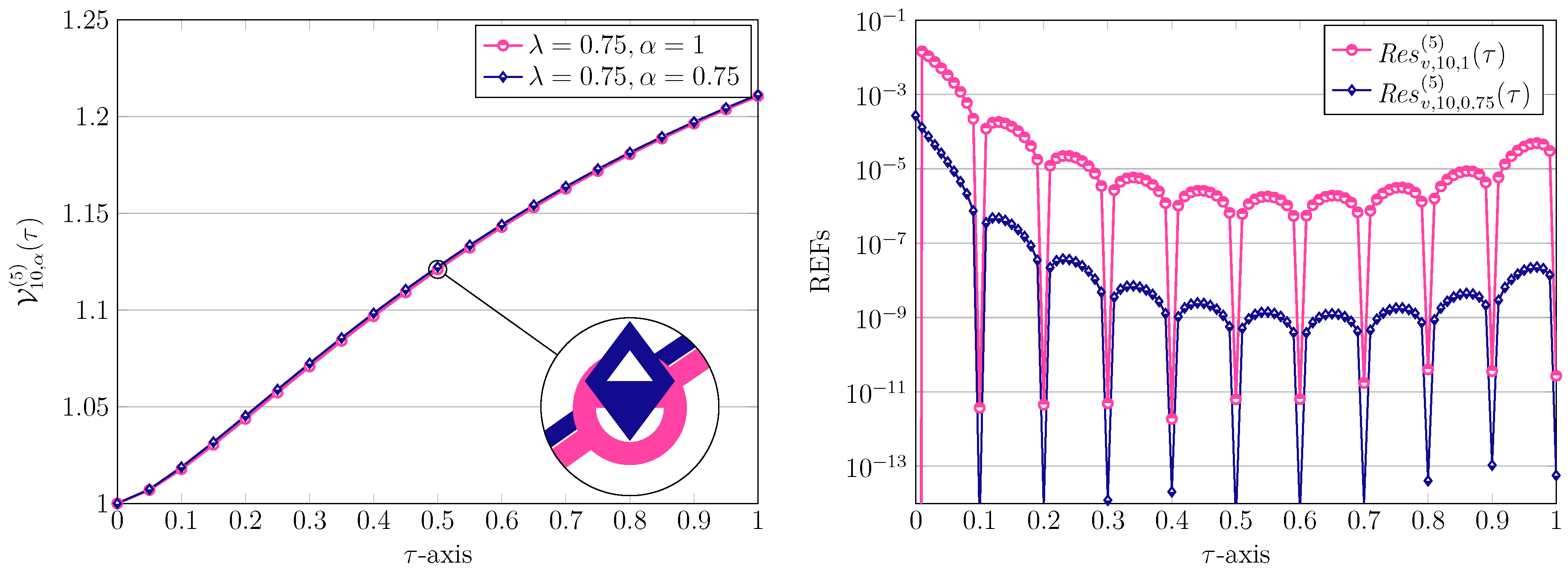
The former approximations for each solution of u ( τ ) and v ( τ ) related to two different values of α = 1 and α = 0.75 are depicted in Figure 3 and Figure 4. In addition to the approximate solutions, we also visualize the associated REFs for each solution on the left plots. By looking at these figures, we infer that the approximate solutions related to both α = 1 , 0.75 are very close together. However, the achieved REFs for α = 0.75 equal to the fractional order λ = 0.75 are smaller in magnitude than those obtained using α = 1 . Therefore, in the next experiments, we only consider the results obtained related to α = λ .
Next, we consider λ = 0.5 and R = 10 . Using α = 0.5 , the approximate solutions evaluated at some point τ [ 0 , 1 ] are reported in Table 3. The corresponding absolute errors defined via relations (35) are also tabulated in Table 3.
When λ = 0.98 , different numerical methods, such as the variational iteration method (VIM) [14], the PLSM [15], the method based on an operational matrix of Bernstein polynomials [16], and LWOMM [17], reported the approximate solutions for this value. In all of these approaches, the solutions obtained are three-degree polynomials. However, here, we first consider the case α = 1 and obtain the following approximate solutions
U 5 , 1 ( 5 ) ( τ ) = 0.038196735 τ 5 0.20054309 τ 4 + 0.32635768 τ 3 + 0.13961269 τ 2 1.054247 τ + 1.0, V 5 , 1 ( 5 ) ( τ ) = 0.03637521 τ 5 + 0.2145241 τ 4 0.5073211 τ 3 + 0.5049069 τ 2 + 0.008199928 τ + 1.0.
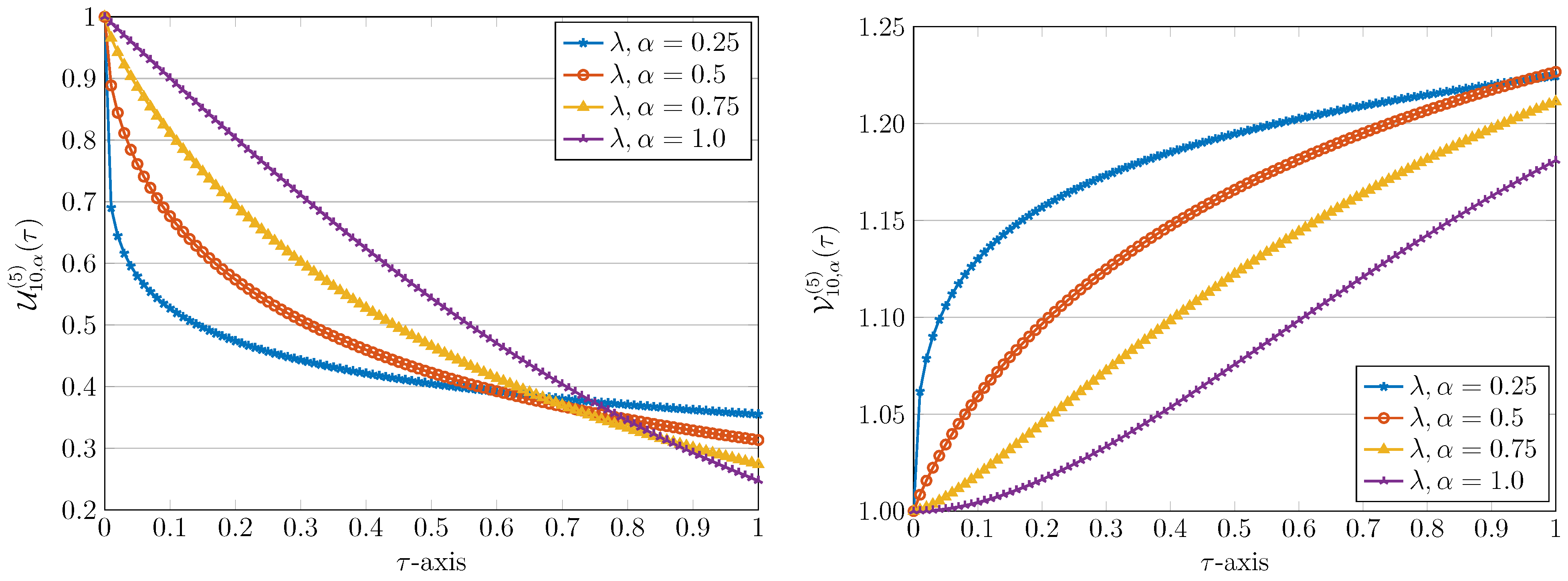
Additionally, the maximum absolute values of REFs using α = 0.98 are shown in Table 4 for various values of R as a power of 2. The related Nocs are also tabulated in this table. Moreover, we present the numerical results when λ , α = 0.75 in Table 4. One can obviously observe a high order of accuracy for the proposed QLM-GCFs. Finally, for the first test case, we use various values of λ = 0.25, 0.5 , 0.75 , 1 . Utilizing R = 10 and α = λ , we plot the numerical solutions in Figure 5.
Example 2.
In the second model problem, we take θ = 0.5 and η = 0.1 . In this case, we consider the nonlinear coupled system
LC D τ λ u ( τ ) = 0.5 1.1 u ( τ ) + u 2 ( τ ) v ( τ ) , LC D τ λ v ( τ ) = 0.1 u ( τ ) u 2 ( τ ) v ( τ ) , λ ( 0 , 1 ] .
Here, we use initial conditions u ( 0 ) = 0.4, v ( 0 ) = 1.5 . This example was considered in [14,16,17] previously.
Let us first take λ , α = 1 . By using R = 5 , the results of the approximations are as follows
U 5 , 1 ( 5 ) ( τ ) = 0.002595532 τ 5 0.01516870 τ 4 + 0.02354928 τ 3 0.002285779 τ 2 + 0.30026 τ + 0.4, V 5 , 1 ( 5 ) ( τ ) = 0.007186591 τ 5 + 0.007075174 τ 4 0.02123004 τ 3 0.1484152 τ 2 0.2001643 τ + 1.5.
The REFs related to the above approximate solutions are shown in Figure 6. To show that the achieved REFs are decreasing as a function of R, we also plot the REFs related to R = 10 , 15 in Figure 6. Clearly, the desired level of accuracy is achievable by increasing the number of basis functions.
We next tabulate the numerical results obtained by using R = 10 in Table 5. Here, we have used the midpoints 0.05, 0.15, , 0.95 on the interval [ 0 , 1 ] . Note that these midpoints are different from the points used in Table 1, which are exactly the same as the collocation points (29) when R = 10 . In fact, the smallest magnitude of errors is achieved at the collocation points. Finally, for this test case and for λ = 1 , we display the maximum absolute REFs achieved by utilizing various R numbers in Table 6. The associated Nocs are also visible in this table. The results show the exponential behavior in terms of the accuracy of the presented QLM-GCFs.
We now consider the fractional-order 0 < λ < 1 . By considering λ = 0.5 , 0.75 , we obtain the results of absolute values of REFs using various R = 2 , 4 , , 32 , as shown in Table 7. The associated numerical order of convergence, i.e., Nocs, is also depicted in Table 7. Obviously, we can get a higher order accuracy by increasing R. Finally, we present numerical results computed at some points τ [ 0 , 1 ] in Table 8. Here, we have used diverse values of λ , α = 0.25, 0.5 , 0.75 .

6. Conclusions

Generalized (fractional-order) clique basis functions (GCFs) have been used to devise not only an effective but also an accurate spectral matrix collocation approach for finding approximate solutions of the nonlinear Brusselator system of equations of fractional order arising in chemical modeling. The fractional derivative is described in the Liouville–Caputo sense. To overcome the underlying nonlinearity of the model, the method of quasi-linearization (QLM) is first employed to receive a family of linearized equations. Afterward, the spectral clique collocation procedure is used to solve this sequence of equations iteratively. The convergence analysis of the proposed combined QLM-GCFs is established. To support the theoretical findings and in order to show the applicability of the QLM-GCFs, a set of numerical test examples is carried out. The results presented in the tables and figures indicate the accuracy of the proposed approach over the existing numerical models and the gain in computational efficiency in terms of CPU time. The presented technique is straightforward, easy to implement, and computationally less demanding.

Author Contributions

Conceptualization, M.I. and H.M.S.; methodology, M.I. and H.M.S.; software, M.I.; validation, M.I. and H.M.S.; formal analysis, M.I. and H.M.S.; funding acquisition, H.M.S.; investigation, M.I. and H.M.S.; writing—original draft preparation, M.I.; writing—review and editing, M.I. and H.M.S. All authors have read and agreed to the published version of the manuscript.

Funding

This research received no external funding.

Institutional Review Board Statement

Not applicable.

Informed Consent Statement

Not applicable.

Data Availability Statement

Not applicable.

Conflicts of Interest

The authors declare no conflict of interest.

References

  1. Prigogine, I.; Lefever, R. Symmetry breaking instabilities in dissipative systems II. J. Chem. Phys. 1968, 48, 1695–1700. [Google Scholar] [CrossRef]
  2. Epstein, I.R.; Pojman, J.K. An Introduction to Nonlinear Chemical Dynamics: Oscillations, Waves, Patterns, and Chaos; Oxford University Press: New York, NY, USA, 1998. [Google Scholar]
  3. Gray, P.; Scott, S.K.; Merkin, J.H. The Brusselator model of oscillatory reactions: Relationships between two-variable and four-variable models with rigorous application of mass conservation and detailed balance. J. Chem. Soc. Faraday Trans. 1988, 84, 993–1011. [Google Scholar] [CrossRef]
  4. Field, R.J.; Györgyi, L. Chaos in Chemistry and Biochemistry; World Scientific: Singapore, 1993. [Google Scholar]
  5. Hilfer, R. (Ed.) Applications of Fractional Calculus in Physics; World Scientific: River Edge, NJ, USA, 2000. [Google Scholar]
  6. Kilbas, A.A.; Srivastava, H.M.; Trujillo, J.J. Theory and Application of Fractional Differential Equations; North-Holland Mathematics Studies: Amsterdam, The Netherllands, 2006; Volume 204. [Google Scholar]
  7. Tong, T.O.; Kekana, M.C.; Shatalov, M.Y.; Moshokoa, S.P. Numerical investigation of Brusselator chemical model by residual function using Mathematica software. J. Comput. Theoret. Nanosci. 2020, 17, 2947–2954. [Google Scholar] [CrossRef]
  8. Gafiychuk, V.; Datsko, B. Stability analysis and limit cycle in fractional system with Brusselator nonlinearities. Phys. Lett. A 2008, 372, 4902–4904. [Google Scholar] [CrossRef]
  9. Sun, M.; Tan, Y.; Chen, L. Dynamical behaviors of the Brusselator system with impulsive input. J. Math. Chem. 2008, 44, 637–649. [Google Scholar] [CrossRef]
  10. Yuan, L.G.; Kuang, J.H. Stability and a numerical solution of fractional-order Brusselator chemical reaction system. J. Fract. Calc. Appl. 2017, 8, 38–47. [Google Scholar]
  11. Wang, Y.; Li, C. Does the fractional Brusselator with efficient dimension less than 1 have a limit cycle? Phys. Lett. A 2007, 363, 414–419. [Google Scholar] [CrossRef]
  12. Ongun, M.Y.; Arslan, D.; Garrappa, R. Nonstandard finite difference schemes for a fractional-order Brusselator system. Adv. Differ. Equ. 2013, 2013, 102. [Google Scholar] [CrossRef] [Green Version]
  13. Zafar, Z.U.A.; Rehan, K.; Mushtaq, M.; Rafiq, M. Numerical treatment for nonlinear Brusselator chemical model. J. Differ. Equ. Appl. 2017, 23, 521–538. [Google Scholar] [CrossRef]
  14. Jafari, H.; Kadem, A.; Baleanu, D. Variational iteration method for a fractional-order Brusselator system. Abstr. Appl. Anal. 2014, 2014, 496323. [Google Scholar] [CrossRef] [Green Version]
  15. Bota, C.; Caruntu, B. Approximate analytical solutions of the fractional-order Brusselator system using the polynomial least squares method. Adv. Math. Phys. 2015, 2015, 450235. [Google Scholar] [CrossRef]
  16. Khan, H.; Jafari, H.; Khan, R.A.; Tajadodi, H.; Johnston, S.J. Numerical solutions of the nonlinear fractional-order Brusselator system by Bernstein polynomials. Sci. World J. 2014, 2014, 257484. [Google Scholar] [CrossRef] [PubMed] [Green Version]
  17. Chang, P.; Isah, A. Legendre wavelet operational matrix of fractional derivative through wavelet-polynomial transformation and its applications in solving fractional order Brusselator system. J. Phys. Conf. Ser. 2016, 693, 012001. [Google Scholar] [CrossRef] [Green Version]
  18. Ongun, M.Y.; Arslan, D.; Farzi, J. Numerical solutions of fractional order autocatalytic chemical reaction model. Süleyman Demirel Ünivers. Fen Bilim. Enstitüsü Dergisi 2017, 21, 165–172. [Google Scholar] [CrossRef]
  19. Asv, R.K.; Devi, S. A novel three-step iterative approach for oscillatory chemical reactions of fractional Brusselator model. Int. J. Model. Simul. 2022, 204, 1–20. [Google Scholar] [CrossRef]
  20. Saad, K.M. Fractal-fractional Brusselator chemical reaction. Chaos Solit. Fract. 2021, 150, 11187. [Google Scholar] [CrossRef]
  21. Mohammadi, M.; Mokhtari, R.; Schaback, R. A meshless method for solving the 2D Brusselator reaction-diffusion system. Comput. Model. Eng. Sci. 2014, 101, 113–138. [Google Scholar]
  22. Tlidi, M.; Gandica, Y.; Sonnino, G.; Averlant, E.; Panajotov, K. Self-Replicating spots in the Brusselator model and extreme events in the one-dimensional case with delay. Entropy 2016, 18, 64. [Google Scholar] [CrossRef] [Green Version]
  23. Alfifi, H.Y. Feedback control for a diffusive and delayed Brusselator model: Semi-analytical solutions. Symmetry 2021, 13, 725. [Google Scholar] [CrossRef]
  24. Mittal, A.K.; Balyan, L.K. A highly accurate time–space pseudospectral approximation and stability analysis of two dimensional Brusselator model for chemical systems. Int. J. Appl. Comput. Math. 2019, 5, 140. [Google Scholar] [CrossRef]
  25. Izadi, M.; Samei, M.E. Time accurate solution to Benjamin-Bona-Mahony Burgers equation via Taylor-Boubaker series scheme. Bound. Value Probl. 2022, 2022, 17. [Google Scholar] [CrossRef]
  26. Razavi, M.; Hosseini, M.M.; Salemi, A. Error analysis and Kronecker implementation of Chebyshev spectral collocation method for solving linear PDEs. Comput. Methods Differ. Equ. 2022, 10, 914–927. [Google Scholar]
  27. Izadi, M.; Srivastava, H.M.; Adel, W. An effective approximation algorithm for second-order singular functional differential equations. Axioms 2022, 11, 133. [Google Scholar] [CrossRef]
  28. Chouhan, D.; Mishra, V.; Srivastava, H.M. Bernoulli wavelet method for numerical solution of anomalous infiltration and diffusion modeling by nonlinear fractional differential equations of variable order. Results Appl. Math. 2021, 10, 100146. [Google Scholar] [CrossRef]
  29. Izadi, M.; Srivastava, H.M. An efficient approximation technique applied to a non-linear Lane-Emden pantograph delay differential model. Appl. Math. Comput. 2021, 401, 126123. [Google Scholar] [CrossRef]
  30. Yüzbaşı, Ş.; Izadi, M. Bessel-quasilinearization technique to solve the fractional-order HIV-1 infection of CD4+ T-cells considering the impact of antiviral drug treatment. Appl. Math. Comput. 2022, 431, 127319. [Google Scholar] [CrossRef]
  31. Srivastava, H.M. Some parametric and argument variations of the operators of fractional calculus and related special functions and integral transformations. J. Nonlinear Convex Anal. 2021, 22, 1501–1520. [Google Scholar]
  32. Srivastava, H.M. An introductory overview of fractional-calculus operators based upon the Fox-Wright and related higher transcendental functions. J. Adv. Eng. Comput. 2021, 5, 135–166. [Google Scholar] [CrossRef]
  33. Hoede, C.; Li, X. Clique polynomials and independent set polynomials of graphs. Discrete Math. 1994, 125, 219–228. [Google Scholar] [CrossRef] [Green Version]
  34. Kumbinarasaiah, S. A new approach for the numerical solution for the non-linear Klein–Gordon equation. SeMA J. 2020, 77, 435–456. [Google Scholar] [CrossRef]
  35. Ganji, R.M.; Jafari, H.; Kgarose, M.; Mohammadi, A. Numerical solutions of time-fractional Klein-Gordon equations by clique polynomials. Alexandria Eng. J. 2021, 60, 4563–4571. [Google Scholar] [CrossRef]
  36. Adel, W.; Kumbinarasaiah, S. A new clique polynomial approach for fractional partial differential equations. Int. J. Nonlinear Sci. Numer. Simul. 2022. [Google Scholar] [CrossRef]
  37. Heydari, M.H.; Razzaghi, M. Highly accurate solutions for space-time fractional Schrödinger equations with non-smooth continuous solution using the hybrid clique functions. Math. Sci. 2021. [Google Scholar] [CrossRef]
  38. Stewart, G.W. Afternotes on Numerical Analysis; SIAM: Philadephia, PA, USA, 1996; Volume 49. [Google Scholar]
  39. Yuttanan, B.; Razzaghi, M.; Vo, T.N. A fractional-order generalized Taylor wavelet method for nonlinear fractional delay and nonlinear fractional pantograph differential equations. Math. Methods Appl. Sci. 2021, 44, 4156–4175. [Google Scholar] [CrossRef]
  40. Izadi, M. An approximation technique for first Painlevé equation. TWMS J. Appl. Eng. Math. 2021, 11, 739–750. [Google Scholar]
  41. Izadi, M.; Yüzbası, Ş.; Noeiaghdam, S. Approximating solutions of non-linear Troesch’s problem via an efficient quasi-linearization Bessel approach. Mathematics 2021, 9, 1841. [Google Scholar] [CrossRef]
  42. Srivastava, H.M.; Shah, F.A.; Irfan, M. Generalized wavelet quasi-linearization method for solving population growth model of fractional order. Math. Methods Appl. Sci. 2020, 43, 8753–8762. [Google Scholar] [CrossRef]
  43. Izadi, M.; Srivastava, H.M. Generalized Bessel quasilinearlization technique applied to Bratu and Lane-Emden type equations of arbitrary order. Fractal Fract. 2021, 5, 179. [Google Scholar] [CrossRef]
  44. Izadi, M.; Yüzbaşı, Ş.; Adel, W. A new Chelyshkov matrix method to solve linear and nonlinear fractional delay differential equations with error analysis. Math. Sci. 2022. [Google Scholar] [CrossRef]
  45. Izadi, M.; Srivastava, H.M. A novel matrix technique for multi-order pantograph differential equations of fractional order. Proc. R. Soc. Lond. Ser. A Math. Phys. Eng. Sci. 2021, 477, 2021031. [Google Scholar] [CrossRef]
  46. Izadi, M.; Yüzbaşı, Ş.; Cattani, C. Approximating solutions to fractional-order Bagley-Torvik equation via generalized Bessel polynomial on large domains. Ricerche Mat. 2021. [Google Scholar] [CrossRef]
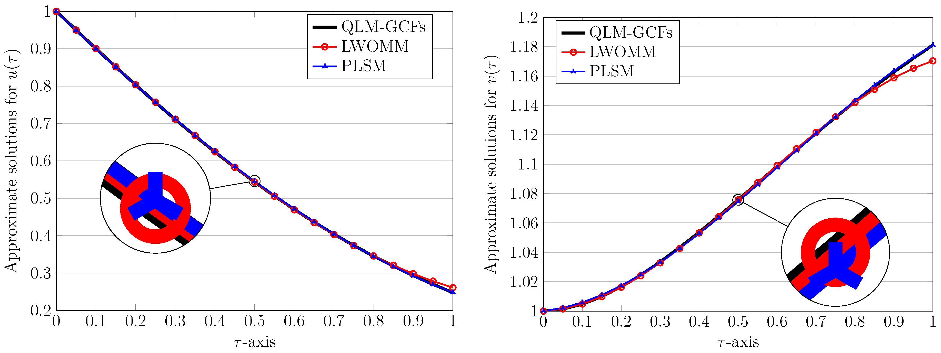
Figure 1. Comparisons of approximate solutions for u ( τ ) (left) and v ( τ ) (right) obtained via the QLM-GCFs technique in test case 1 with R = 5 , λ , α = 1 , and p = 5 .
Axioms 11 00654 g001
Figure 2. Comparisons of achieved REFs obtained via QLM-GCFs in test case 1 with λ , α = 1 , R = 5 , 10 , 15 , and p = 5 .
Axioms 11 00654 g002
Figure 3. Comparisons of approximate solutions for u ( τ ) (left) and related REFs (right) obtained via the QLM-GCFs technique in Example 1 with R = 10 , λ = 0.75, α = 1 , 0.75 , and p = 5 .
Axioms 11 00654 g003
Figure 4. Comparisons of approximate solutions for v ( τ ) (left) and related REFs (right) obtained via the QLM-GCFs technique in Example 1 with R = 10 , λ = 0.75, α = 1 , 0.75 , and p = 5 .
Axioms 11 00654 g004
Figure 5. Comparisons of approximate solutions for u ( τ ) (left) and v ( τ ) (right) obtained via the QLM-GCFs technique in Example 1 with R = 10 , λ , α = 0.25, 0.5 , 0.75, 1 , and p = 5 .
Axioms 11 00654 g005
Figure 6. Comparisons of achieved REFs obtained via QLM-GCFs in Example 2 with λ , α = 1 , R = 5 , 10 , 15 , and p = 5 .
Axioms 11 00654 g006
Table 1. Numerical results and REFs for u ( τ ) , v ( τ ) obtained via the QLM-GCFs procedure using R = 10 and p = 5 in Example 1 with λ , α = 1 .
τ U 10 , 1 ( 5 ) ( τ ) Res u , 10 , 1 ( 5 ) ( τ ) V 10 , 1 ( 5 ) ( τ ) Res v , 10 , 1 ( 5 ) ( τ )
0.1 0.900464302493772 2.7735 × 10 15 1.004523943044246 4.6810 × 10 15
0.2 0.803448542998189 1.1723× 10 15 1.016373836862601 8.9920× 10 15
0.3 0.710824317213952 1.2023× 10 14 1.033327205646229 1.3351× 10 15
0.4 0.623892736413153 1.1641× 10 14 1.053574529276645 1.0168× 10 14
0.5 0.543504717634733 1.3233× 10 16 1.075649740696301 1.0648× 10 14
0.6 0.470149961736370 1.2558× 10 14 1.098381593278497 2.8102× 10 14
0.7 0.404024163774677 3.7396× 10 14 1.120859071635027 1.4690× 10 14
0.8 0.345083563213368 3.6526× 10 14 1.142403440455486 2.1380× 10 14
0.9 0.293093303881749 8.6498× 10 14 1.162541379315871 5.4074× 10 14
1.0 0.247672792516836 7.3249× 10 14 1.180976444182846 4.0555× 10 14
Table 2. The results of L norms, the corresponding convergence rate, and CPU times in Example 1 with diverse R, λ , α = 1 , and p = 5 .
R L u Noc u L v Noc v CPU(s)
2 8.8464× 10 2 2.5585× 10 1 0.55877
4 2.3798× 10 2 1.8942 1.4707× 10 2 4.1207 0.83877
8 9.2239× 10 5 8.0113 1.1027× 10 4 7.0593 1.64742
16 1.0027× 10 8 13.167 1.0748× 10 8 13.325 3.67631
32 3.1173× 10 11 8.3294 6.7817× 10 11 7.3082 9.55585
Table 3. Numerical results and REFs for u ( τ ) , v ( τ ) obtained via the QLM-GCFs procedure using R = 10 , p = 5 in Example 1 with λ , α = 0.5 .
τ U 10 , 0.5 ( 5 ) ( τ ) Res u , 10 , 0.5 ( 5 ) ( τ ) V 10 , 0.5 ( 5 ) ( τ ) Res v , 10 , 0.5 ( 5 ) ( τ )
0.1 0.676592310003481 2.8530× 10 14 1.059227208815533 1.4962× 10 15
0.2 0.573857423802071 1.1549× 10 13 1.096675293835927 1.0566× 10 13
0.3 0.507770381824183 1.3181× 10 13 1.124827045650820 1.3320× 10 13
0.4 0.459738270417381 6.8264× 10 13 1.147290159849651 2.6591× 10 13
0.5 0.422579704301791 1.0439× 10 13 1.165852096005718 1.5040× 10 13
0.6 0.392675915528585 4.1750× 10 13 1.181563743233397 4.5923× 10 14
0.7 0.367932268722878 9.3469× 10 13 1.195103916669479 4.5888× 10 14
0.8 0.347025860146580 7.5152× 10 13 1.206938751776391 1.2845× 10 13
0.9 0.329068932537851 3.1123× 10 14 1.217402627420391 7.1534× 10 14
1.0 0.313438314355603 1.2928× 10 12 1.226743490360364 1.1390× 10 13
Table 4. The results of L norms, the corresponding convergence rate in Example 1 with diverse R, λ , α = 0.75, 0.98 , and p = 5 .
λ = 0.75 λ = 0.98
R L u Noc u L v Noc v L u Noc u L v Noc v
2 2.9301 02 2.6438 01 8.4327 02 2.5731 01
4 6.7159 02 1.1966 5.1045 02 2.3727 2.6363 02 1.6775 1.6514 02 3.9617
8 5.9544 04 6.8175 3.7342 04 7.0948 9.6808 05 8.0892 1.2087 04 7.0941
16 8.0008 07 9.5396 5.8560 07 9.3167 1.5261 08 12.631 1.5225 08 12.955
32 2.3658 08 5.0797 1.2673 08 5.5301 4.7902 11 8.3155 2.3028 11 9.3689
Table 5. Numerical results and REFs for u ( τ ) , v ( τ ) obtained via the QLM-GCFs procedure using R = 10 , p = 5 in Example 2 with λ , α = 1 .
τ U 10 , 1 ( 5 ) ( τ ) Res u , 10 , 1 ( 5 ) ( τ ) V 10 , 1 ( 5 ) ( τ ) Res v , 10 , 1 ( 5 ) ( τ )
0.05 0.420364987163538 5.4281× 10 08 1.464193736210683 6.9171× 10 08
0.15 0.458172247718453 2.8803× 10 09 1.395407097431014 3.6639× 10 09
0.25 0.492300715744509 5.0979× 10 10 1.330238068232444 6.4809× 10 10
0.35 0.523000098574405 1.6945× 10 10 1.268512980921797 2.1555× 10 10
0.45 0.550506819287693 9.0387× 10 11 1.210065493419779 1.1521× 10 10
0.55 0.575044582788486 7.2710× 10 11 1.154736326110934 9.3018× 10 11
0.65 0.596824922738173 8.6618× 10 11 1.102373006480542 1.1144× 10 10
0.75 0.616047729841562 1.5522× 10 10 1.052829621356641 2.0132× 10 10
0.85 0.632901761975499 4.4405× 10 10 1.005966576578516 5.8234× 10 10
0.95 0.647565136639679 2.3660× 10 09 0.961650363916099 3.1497× 10 09
Table 6. The results of L norms, the corresponding convergence rate, and CPU times in Example 2 with diverse R, λ , α = 1 , and p = 5 .
R L u Noc u L v Noc v
2 2.3453× 10 2 3.1850× 10 2
4 1.5211× 10 3 3.9466 3.7107× 10 3 3.1015
8 1.5652× 10 6 9.9245 3.1978× 10 7 13.502
16 3.8244× 10 11 15.321 5.1169× 10 11 12.610
32 4.0160× 10 13 6.5733 5.1238× 10 14 9.9638
Table 7. The results of L norms and the corresponding convergence rate in Example 2 with diverse R, λ , α = 0.5 , 0.75 , and p = 5 .
λ = 0.5 λ = 0.75
R L u Noc u L v Noc v L u Noc u L v Noc v
2 8.3797 02 1.7867 01 6.2299 02 1.0729 01
4 5.0780 02 0.7226 6.4041 02 1.4802 4.2712 02 3.8665 3.0414 03 5.1406
8 5.6280 03 3.1736 3.8246 03 4.0656 4.1380 04 3.3676 5.3709 04 2.5015
16 1.2860 04 5.4516 4.9033 05 6.2854 6.9800 08 12.533 6.5807 08 12.995
32 1.8406 07 9.4485 3.9839 07 6.9434 1.1363 11 12.585 4.3433 11 10.565
Table 8. Numerical results and REFs for u ( τ ) , v ( τ ) obtained via the QLM-GCFs procedure using R = 10 , p = 5 in Example 2 with λ , α = 0.25, 0.5 , 0.75 .
λ = α = 0.25 λ = α = 0.5 λ = α = 0.75
τ U 10 , α ( 5 ) ( τ ) V 10 , α ( 5 ) ( τ ) U 10 , α ( 5 ) ( τ ) V 10 , α ( 5 ) ( τ ) U 10 , α ( 5 ) ( τ ) V 10 , α ( 5 ) ( τ )
0.05 0.53635357 1.36264701 0.54865158 1.35823553 0.47111143 1.40197516
0.15 0.59116199 1.26326681 0.62140849 1.25622929 0.54574688 1.28946276
0.25 0.61628002 1.20991192 0.65785082 1.18993711 0.59572321 1.20586462
0.35 0.63187140 1.17308734 0.68077488 1.13917346 0.63266615 1.13749235
0.45 0.64277275 1.14501830 0.69648157 1.09776992 0.66096850 1.07937071
0.55 0.65091723 1.12240609 0.70772186 1.06280079 0.68300039 1.02887191
0.65 0.65726824 1.10352709 0.71595859 1.03259028 0.70025234 0.98436225
0.75 0.66237220 1.08736331 0.72206423 1.00606805 0.71374714 0.94472572
0.85 0.66656700 1.07326219 0.72660021 0.98249967 0.72422723 0.90915154
0.95 0.67007499 1.06078003 0.72994787 0.96135501 0.73225308 0.87702453
Publisher’s Note: MDPI stays neutral with regard to jurisdictional claims in published maps and institutional affiliations.