


RETRACTED: Diabetic Retinopathy Progression Prediction Using a Deep Learning Model

Abstract
:1. Introduction
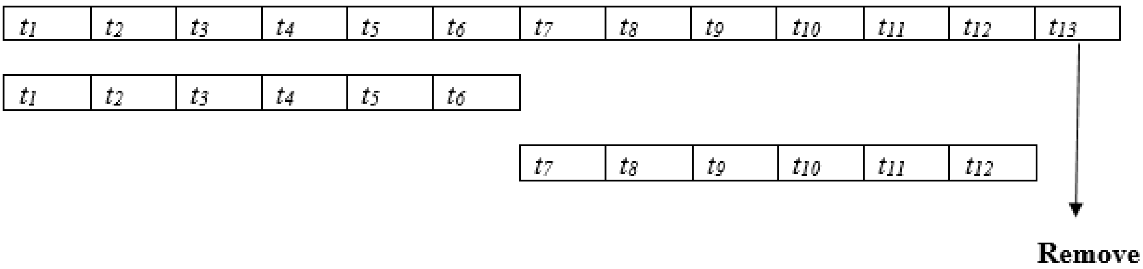
- The temporal representations of the ocular cases are taken in seven successive visual field tests over 4.3 years to test the progression of the disease and predict the progression using deep learning.
- The overall accuracy is improved compared to the related work.
2. Dataset
2.1. Random Errors and Fluctuations to Visual Field Tests
2.2. Training and Testing Dataset
2.3. Visual Field Test
2.4. Convolutional Neural Network
- A.
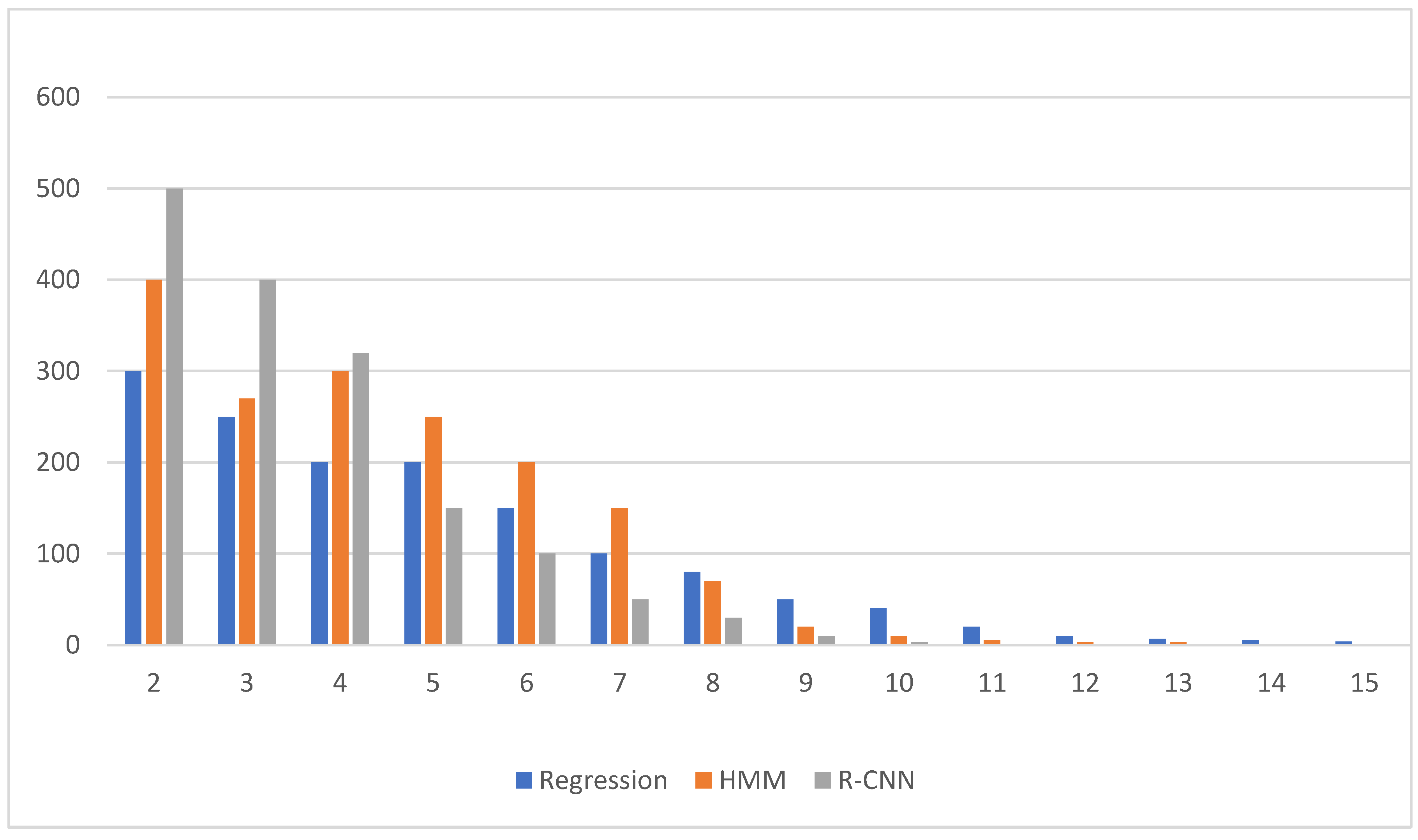
- HMM and R-CNN
- B.
- Proposed Model and Experimental Results
3. Experiments
3.1. Experimental Results Analyses
3.2. Experimental Results
4. Conclusions
Funding
Acknowledgments
Conflicts of Interest
References
- Resnikoff, S.; Pascolini, D.; Etya’Ale, D.; Kocur, I.; Pararajasegaram, R.; Pokharel, G.P.; Mariotti, S.P. Global data on visual impairment in the year 2002. Bull. World Health Organ. 2004, 9, 844–851. [Google Scholar]
- Weinreb, R.N.; Aung, T.; Medeiros, F.A. The Pathophysiology and Treatment of Diabetic retinopathy: A Review. JAMA 2014, 311, 1901. [Google Scholar] [CrossRef]
- Henson, D.B.; Chaudry, S.; Artes, P.H.; Faragher, E.B.; Ansons, A. Response Variability in the Visual Field: Comparison of Optic Neuritis, Diabetic retinopathy, Ocular Hypertension, and Normal Eyes. Investig. Ophthalmol. Vis. Sci. 2000, 41, 5. [Google Scholar]
- Wang, M.; Shen, L.Q.; Pasquale, L.R.; Petrakos, P.; Formica, S.; Boland, M.V.; Wellik, S.R.; De Moraes, C.G.; Myers, J.S.; Saeedi, O.; et al. An Artificial Intelligence Approach to Detect Visual Field Progression in Diabetic retinopathy Based on Spatial Pattern Analysis. Investig. Ophthalmol. Vis. Sci. 2019, 60, 365. [Google Scholar] [CrossRef] [PubMed]
- Murata, H.; Araie, M.; Asaoka, R. A New Approach to Measure Visual Field Progression in Diabetic retinopathy Ocular cases Using Variational Bayes Linear Regression. Investig. Ophthalmol. Vis. Sci. 2014, 55, 8386–8392. [Google Scholar] [CrossRef]
- Wen, J.C.; Lee, C.S.; Keane, P.A.; Xiao, S.; Rokem, A.S.; Chen, P.P.; Wu, Y.; Lee, A.Y. Forecasting progressive Humphrey Visual Fields using deep learning. PLoS ONE 2019, 14, e0214875. [Google Scholar] [CrossRef] [PubMed]
- Berchuck, S.I.; Mukherjee, S.; Medeiros, F.A. Estimating Rates of Progression and Predicting Progressive Visual Fields in Diabetic retinopathy Using a Deep Variational Autoencoder. Sci. Rep. 2019, 9, 18113. [Google Scholar] [CrossRef]
- Jun, T.J.; Eom, Y.; Kim, D.; Kim, C.; Park, J.H.; Nguyen, H.M.; Kim, D. TRk-CNN: Transferable ranking-CNN for image classification of glaucoma, glaucoma suspect, and normal eyes. Expert Syst. Appl. 2021, 182, 115211. [Google Scholar] [CrossRef]
- Manias, G.; Kiourtis, A.; Mavrogiorgou, A.; Kyriazis, D. Multilingual Sentiment Analysis on Twitter Data Towards Enhanced Policy Making. In Proceedings of the IFIP International Conference on Artificial Intelligence Applications and Innovations, León, Spain, 14–17 June 2022; Springer: Cham, Switzerland, 2022; pp. 325–337. [Google Scholar]
- Kattenborn, T.; Leitloff, J.; Schiefer, F.; Hinz, S. Review on Convolutional Neural Networks (CNN) in vegetation remote sensing. ISPRS J. Photogramm. Remote Sens. 2021, 173, 24–49. [Google Scholar] [CrossRef]
- Salehinejad, H.; Sankar, S.; Barfett, J.; Colak, E.; Valaee, S. Recent Advances in Recurrent Neural Networks. arXiv 2017, arXiv:1801.01078. [Google Scholar]
- Liu, S.; Yang, N.; Li, M.; Zhou, M. A Recursive Recurrent Neural Network for Statistical Machine Translation. In Proceedings of the 52nd Annual Meeting of the Association for Computational Linguistics, Baltimore, MD, USA, 22–27 June 2014; Volume 1, pp. 1491–1500. [Google Scholar]
- Young, T.; Hazarika, D.; Poria, S.; Cambria, E. Recent Trends in Deep Learning Based Natural Language Processing. IEEE Comput. Intell. Mag. 2018, 13, 55–75. [Google Scholar] [CrossRef]
- Hochreiter, S.; Schmidhuber, J. Long Short-Term Memory. Neural Comput. 1997, 9, 1735–1780. [Google Scholar] [CrossRef] [PubMed]
- Chung, J.; Gulcehre, C.; Cho, K.; Bengio, Y. Empirical Evaluation of Gated Recurrent Neural Networks on Sequence Modeling. arXiv 2014, arXiv:1412.3555. [Google Scholar]
- Park, K.; Kim, J.; Lee, J. Visual Field Classification using Recurrent Neural Network. Sci. Rep. 2019, 9, 8385. [Google Scholar] [CrossRef]
- Dixit, A.; Yohannan, J.; Boland, M.V. Assessing Diabetic retinopathy Progression Using Machine Learning Trained on Longitudinal Visual Field and Clinical Data. Ophthalmology 2021, 128, 1016–1026. [Google Scholar] [CrossRef] [PubMed]
- Lynn, H.M.; Pan, S.B.; Kim, P. A Deep Bidirectional R-CNN Network Model for Biometric Electrocardiogram Classification Based on Recurrent Neural Networks. IEEE Access. 2019, 7, 145395–145405. [Google Scholar] [CrossRef]
- Cho, K.; van Merrienboer, B.; Gulcehre, C.; Bahdanau, D.; Bougares, F.; Schwenk, H.; Bengio, Y. Learning Phrase Representations using RNN Encoder–Decoder for Statistical Machine Translation. arXiv 2014, arXiv:1406.1078. [Google Scholar]
- Khandelwal, S.; Lecouteux, B.; Besacier, L. Comparing R-CNN and Hmm For Automatic Speech Recognition; LIG: Indore, India, 2016. [Google Scholar]
- Li, X.; Li, X.; Ma, X.; Xiao, F.; Xiao, C.; Wang, F.; Zhang, S. Time-series production forecasting method based on the integration of Bidirectional Gated Recurrent CNN (R-CNN) network and Sparrow Search Algorithm (SSA). J. Pet. Sci. Eng. 2022, 208, 109309. [Google Scholar] [CrossRef]
- Darmawahyuni, A.; Nurmaini, S.; Rachmatullah, M.N.; Firdaus, F.; Tutuko, B. Unidirectional-bidirectional recurrent networks for cardiac disorders classification. Telkomnika 2021, 19, 902. [Google Scholar] [CrossRef]
- Schuster, M.; Paliwal, K.K. Bidirectional recurrent neural networks. IEEE Trans. Signal Process. 1997, 45, 2673–2681. [Google Scholar] [CrossRef]
- Ferreira, J.; Júnior, A.A.; Galvão, Y.M.; Barros, P.; Fernandes, S.M.M.; Fernandes, B.J. Performance Improvement of Path Planning algorithms with Deep Learning Encoder Model. In Proceedings of the 2020 Joint IEEE 10th International Conference on Development and Learning and Epigenetic Robotics (ICDL-EpiRob), Valparaiso, Chile, 26–30 October 2020; pp. 1–6. [Google Scholar]
- Pascanu, R.; Gulcehre, C.; Cho, K.; Bengio, Y. How to Construct Deep Recurrent Neural Networks. arXiv 2013, arXiv:1312.6026. [Google Scholar]
- Gomes, J.C.; Masood, A.I.; Silva, L.H.d.S.; da Cruz Ferreira, J.R.B.; Júnior, A.A.F.; dos Santos Rocha, A.L.; de Oliveira, L.C.P.; da Silva, N.R.C.; Fernandes, B.J.T.; Dos Santos, W.P. COVID-19 diagnosis by combining RT-PCR and pseudo-convolutional machines to characterize virus sequences. Sci. Rep. 2021, 11, 1–28. [Google Scholar]
- Majumder, S.; Elloumi, Y.; Akil, M.; Kachouri, R.; Kehtarnavaz, N. A deep learning-based smartphone app for real-time detection of five stages of diabetic retinopathy. In Real-Time Image Processing and Deep Learning 2020; International Society for Optics and Photonics; SPIE: Bellingham, WA, USA, 2020; Volume 11401, p. 1140106. [Google Scholar]
- Asaoka, R.; Murata, H.; Iise, A.; Araie, M. Detecting Preperimetric Diabetic retinopathy with Standard Automated Perimetry Using a Deep Learning Classifier. Ophthalmology 2016, 123, 1974–1980. [Google Scholar] [CrossRef] [PubMed]
- Garway-Heath, D.F.; Poinoosawmy, D.; Fitzke, F.W.; Hitchings, R.A. Mapping the Visual Field to the Optic Disc in Normal Tension Diabetic retinopathy Eyes. Ophthalmology 2000, 107, 7. [Google Scholar]
- Silva, L.H.d.S.; George, O.d.A.; Fernandes, B.J.; Bezerra, B.L.; Lima, E.B.; Oliveira, S.C. Automatic Optical Inspection for Defective PCB Detection Using Transfer Learning. In Proceedings of the 2019 IEEE Latin American Conference on Computational Intelligence (LA-CCI), Guayaquil, Ecuador, 11–15 November 2019; pp. 1–6. [Google Scholar]
- Borrelli, E.; Sacconi, R.; Querques, L.; Battista, M.; Bandello, F.; Querques, G. Quantification of diabetic macular ischemia using novel three-dimensional optical coherence tomography angiography metrics. J. Biophotonics 2020, 13, e202000152. [Google Scholar] [CrossRef]
- Zang, P.; Gao, L.; Hormel, T.T.; Wang, J.; You, Q.; Hwang, T.S.; Jia, Y. DcardNet: Diabetic retinopathy classification at multiple levels based on structural and angiographic optical coherence tomography. IEEE Trans. Biomed. Eng. 2020, 68, 1859–1870. [Google Scholar] [CrossRef]
- Ayala, A.; Ortiz Figueroa, T.; Fernandes, B.; Cruz, F. Diabetic Retinopathy Improved Detection Using Deep Learning. Appl. Sci. 2021, 11, 11970. [Google Scholar] [CrossRef]
- Dai, L.; Wu, L.; Li, H.; Cai, C.; Wu, Q.; Kong, H.; Liu, R.; Wang, X.; Hou, X.; Liu, Y.; et al. A deep learning system for detecting diabetic retinopathy across the disease spectrum. Nat. Commun. 2021, 12, 3242. [Google Scholar] [CrossRef]
- Lyu, X.; Jajal, P.; Tahir, M.Z.; Zhang, S. Fractal dimension of retinal vasculature as an image quality metric for automated fundus image analysis systems. Sci. Rep. 2022, 12, 11868. [Google Scholar] [CrossRef]
- Pour, E.K.; Rezaee, K.; Azimi, H.; Mirshahvalad, S.M.; Jafari, B.; Fadakar, K.; Faghihi, H.; Mirshahi, A.; Ghassemi, F.; Ebrahimiadib, N.; et al. Automated machine learning–based classification of proliferative and non-proliferative diabetic retinopathy using optical coherence tomography angiography vascular density maps. Graefes Arch. Clin. Exp. Ophthalmol. 2022. [Google Scholar] [CrossRef]


| Reference | Research Description | Proposed Solution | Database | Average Accuracy |
|---|---|---|---|---|
| [24] | Deep learning CNN for early detection of stages of diabetic retinopathy | The model uses markers for classification to predict abnormalities by computing features correlation. | 980 Fundus oculi images | 91.5% |
| [25] | Deep learning diagnosis of pre-parametric retinopathy due to diabetes with automated perimetry methodology | Deep learning using Fourier polynomials | Small-sized dataset, cannot be generalized | 91.7% |
| [26] | Cornea classification by mapping visual field of diabetic retinopathy eyes | Pixel-differentiation of the Fundus oculi images | 2000 Fundus oculi images | 91.57% with high recall |
| [27] | Fundus oculi imaging irregularities detection of optical identification of PCB using transfer learning | Intelligent classification model | unknown | 91.7% |
| [28] | Multi-label retinopathy ocular classification of diabetic macular ischemia utilizing 3-D coherence method | Dense neural network | 1300 | 92.5% |
| [29] | Quantifying diabetic retinopathy niches using OCT imaging defining DcardNet: multi— classification at multiple levels based on structural and angiographic of optical retinopathy. | Discrete domain-optical analysis | Fundus oculi image 2100 Fundus oculi images | 87.93% |
| [30] | Deep image CNN for diabetic retinopathy diagnosis. | Feature data mining detection in retinal fundus | 950 Fundus oculi images of five labelled diabetic retinopathy cases | 89.16% |
| [31] | Automated corneal image analysis with the exclusion of areas that does not indicate dangerous disease | Regional CNN | 4130 Fundus oculi images | 90.97% |
| [32] | Progression diabetic retinopathy in corneal fundus oculi videos using the fractal dimension | Image-Net convolutional neural network | 1700 videos with 25 frames each | 88.4% |
| [33] | Deep learning prediction of proliferative diabetic retinopathy employing optical angiography vascular density | Geometric parameters | 1320 3-D Fundus oculi images | 90.7% |
| Our proposed model | A multitasking fusion deep CNN for detecting the progression of diabetic retinopathy phases from no-diabetic retinopathy to severe diabetic retinopathy progression over 4.3 years on average. | 14,000 oculi images | MSE and p-values are used |
| Characteristics | The Whole Dataset | Training Data | Testing Data |
|---|---|---|---|
| Number of ocular cases (each eye) | 14,000 (7000) | 11,200 (5600) | 2800 (1400) |
| Age; average standard deviation | 49.96 16.04 | 44.11 14.88 | 49.19 16.84 |
| Initial field: IF (dB); average standard deviation | −4.89 6.21 | −4.77 6.16 | −6.19 6.44 |
| Follow up (years); average standard deviation | 4.69 2.74 | 4.87 2.87 | 4.61 1.84 |
| Average number of visual field tests | 8.48 2.08 | 8.82 2.22 | 6.00 0.00 |
| IF 6 dB | 4416 | 2688 | 828 |
| 5 dB IF 13 dB | 1218 | 881 | 226 |
| 13 dB IF | 1062 | 846 | 208 |
| Dataset extension | |||
| Cases of the dataset with eight eyes series | 8222 | 8061 | 1282 |
| Follow up (years); average standard deviation | 4.28 1.68 | 4.26 1.66 | 4.61 1.84 |
| Detection time (years); average standard deviation | 0.84 0.82 | 0.82 0.81 | 1.00 0.84 |
| IF 5 dB | 6688 | 4861 | 828 |
| 5 dB IF 13 dB | 1488 | 1241 | 226 |
| 13 dB IF | 1268 | 1068 | 208 |
| Progress in Years | 0 | 2–4 Years | 4–8 Years | 8–12 Years | >12 Years |
|---|---|---|---|---|---|
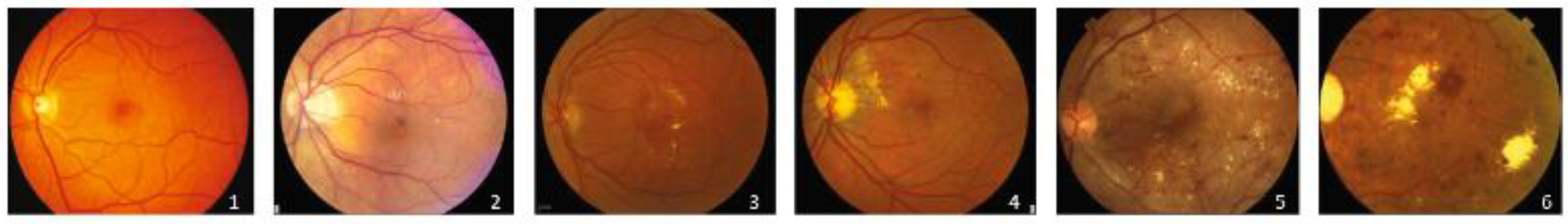
| Class of diabetic retinopathy | Normal | Mild diabetic retinopathy | Moderate diabetic retinopathy | Severe diabetic retinopathy | Proliferate diabetic retinopathy |
| Damage to retina | No retinopathy | Minute alteration in blood vessels. | blood vessels leakage. | Larger blood leakages and. vessel blockage. | Vision loss. |
| Diabetic Retinopathy Class/Count of Images | Training Set | Testing Set | ||
|---|---|---|---|---|
| Left Eye | Right Eye | Left Eye | Right Eye | |
| Normal (No diabetic retinopathy) | 1224 | 1226 | 197 | 203 |
| Mild diabetic retinopathy | 1200 | 1231 | 190 | 189 |
| Moderate diabetic retinopathy | 2102 | 2240 | 395 | 390 |
| Severe diabetic retinopathy | 421 | 448 | 313 | 318 |
| Proliferate diabetic retinopathy | 353 | 355 | 305 | 300 |
| Number of Cases | |
|---|---|
| Total | 2100 |
| Gender, Male (%) | 1092 (52%) |
| Diagnosis | |
| Diabetic retinopathy suspect | 560 |
| Primary open angle diabetic retinopathy | 840 |
| Pseudo exfoliation diabetic retinopathy | 100 |
| Primary angle closure diabetic retinopathy | 299 |
| Secondary diabetic retinopathy | 190 |
| Others | 111 |
| Regression Method | HMM | R-CNN | ANOVA p-Value | p-Value | ||||
|---|---|---|---|---|---|---|---|---|
| Regression Method vs. R-CNN | HMM vs. R-CNN | Regression Method vs. HMM | ||||||
| Prediction error, average standard deviation | MSE (dB) | 5.81 5.89 | 5.06 3.61 | 5.71 3.53 | <0.001 | <0.001 | <0.001 | <0.001 |
| PMAE (dB) | 5.53 0.56 | 5.10 0.59 | 3.80 0.56 | <0.001 | <0.001 | <0.001 | <0.001 | |
| Predicted Cases | Proliferate | |||||
|---|---|---|---|---|---|---|
| Normal | Mild | Moderate | Severe | |||
| Actual Cases |
Normal (No diabetic retinopathy) | 280 | 12 | 8 | 0 | 0 |
|
Mild diabetic retinopathy | 10 | 270 | 15 | 3 | 2 | |
|
Moderate diabetic retinopathy | 1 | 16 | 270 | 10 | 3 | |
|
Severe diabetic retinopathy | 0 | 0 | 3 | 290 | 7 | |
|
Proliferate diabetic retinopathy | 0 | 0 | 2 | 25 | 273 | |
| Predicted Cases | Proliferate | |||||
|---|---|---|---|---|---|---|
| Normal | Mild | Moderate | Severe | |||
| Actual Cases | Normal (No diabetic retinopathy) | 285 | 10 | 5 | 0 | 0 |
|
Mild diabetic retinopathy | 10 | 277 | 8 | 3 | 2 | |
|
Moderate diabetic retinopathy | 1 | 14 | 280 | 5 | 0 | |
|
Severe diabetic retinopathy | 0 | 0 | 0 | 293 | 7 | |
|
Proliferate diabetic retinopathy | 0 | 0 | 1 | 19 | 280 | |
| Predicted Cases | Proliferate | |||||
|---|---|---|---|---|---|---|
| Normal | Mild | Moderate | Severe | |||
| Actual Cases |
Normal (No diabetic retinopathy) | 292 | 8 | 0 | 0 | 0 |
|
Mild diabetic retinopathy | 3 | 293 | 4 | 0 | 0 | |
|
Moderate diabetic retinopathy | 0 | 4 | 290 | 5 | 1 | |
|
Severe diabetic retinopathy | 0 | 0 | 0 | 295 | 5 | |
| Proliferate diabetic retinopathy | 0 | 0 | 0 | 5 | 295 | |
| Prediction Error (MSE, dB), Average Standard Deviation | p-Value | |||||
|---|---|---|---|---|---|---|
| Regression Method | HMM | R-CNN | R-CNN vs. HMM | R-CNN vs. Regression Method | Regression Method vs. HMM | |
| Spatial | 4.85 5.08 | 4.39 3.86 | 4.03 3.55 | <0.001 | <0.001 | <0.001 |
| Temporal | 4.94 5.53 | 4.79 4.53 | 4.38 3.91 | <0.001 | <0.001 | 0.310 |
| Intertemporal | 5.58 5.19 | 4.78 4.05 | 4.54 3.85 | <0.001 | <0.001 | <0.001 |
| Nose angle | 5.34 5.75 | 5.30 4.34 | 4.97 4.36 | <0.001 | <0.001 | <0.001 |
| Marginal | 5.90 4.95 | 5.05 3.60 | 4.74 3.58 | <0.001 | <0.001 | <0.001 |
| Dominant | 5.08 5.18 | 4.76 4.15 | 4.44 3.68 | <0.001 | 0.001 | <0.001 |
| Prediction error (MSE, dB), Average ± Standard Deviation | Number of Eyes | p-Value | ||||||
|---|---|---|---|---|---|---|---|---|
| Regression Method | HMM | R-CNN | R-CNN vs. HMM | R-CNN vs. Regression Method | Regression Method vs. HMM | ANOVA | ||
| prediction error vs. false positive rate (FPR, %) | ||||||||
| FP rate ≤ 2 | 5.90 ± 5.43 | 5.06 ± 3.65 | 4.71 ± 3.55 | 797 | <0.001 | <0.001 | <0.001 | <0.001 |
| 2 < FP 5 | 5.75 ± 4.35 | 5.18 ± 3.69 | 4.80 ± 3.54 | 358 | <0.001 | <0.001 | <0.001 | <0.001 |
| 5 < FP 8 | 5.43 ± 3.53 | 4.83 ± 3.48 | 4.53 ± 3.18 | 73 | <0.001 | <0.001 | 0.007 | <0.001 |
| 8 < FP 10.0 | 4.90 ± 3.38 | 4.74 ± 3.14 | 4.45 ± 1.95 | 57 | <0.001 | 0.001 | 0.431 | <0.001 |
| FP rate > 10 | 5.15 ± 4.19 | 5.19 ± 3.54 | 4.85 ± 3.44 | 88 | <0.001 | <0.001 | <0.001 | <0.001 |
| prediction error and false negative (FN rate %) | ||||||||
| FN rate ≤ 2.5 | 5.34 ± 4.88 | 4.58 ± 3.59 | 4.33 ± 3.31 | 766 | <0.001 | <0.001 | <0.001 | <0.001 |
| 2 < FN 5 | 5.16 ± 3.93 | 4.43 ± 1.79 | 4.10 ± 1.59 | 155 | <0.001 | <0.001 | <0.001 | <0.001 |
| 5 < FN 8 | 5.63 ± 4.03 | 5.05 ± 3.41 | 5.57 ± 3.06 | 109 | <0.001 | <0.001 | 0.007 | <0.001 |
| 8 < FN ≤ 10.0 | 5.65 ± 3.91 | 5.53 ± 3.05 | 5.30 ± 1.89 | 91 | <0.001 | <0.001 | <0.001 | <0.001 |
| FN rate > 10 | 7.43 ± 5.67 | 6.36 ± 4.04 | 5.95 ± 4.08 | 151 | <0.001 | <0.001 | <0.001 | <0.001 |
| prediction error vs. loss function (L, %) | ||||||||
| L ≤ 3 | 5.91 ± 5.88 | 5.04 ± 3.75 | 4.66 ± 3.53 | 518 | <0.001 | <0.001 | <0.001 | <0.001 |
| 3 < L ≤ 5 | 6.55 ± 3.99 | 5.99 ± 3.30 | 5.17 ± 3.06 | 14 | 0.003 | 0.035 | 0.533 | <0.001 |
| 5 < L ≤ 8 | 5.59 ± 3.87 | 5.08 ± 3.61 | 4.71 ± 3.48 | 175 | <0.001 | <0.001 | 0.001 | <0.001 |
| 8 < L ≤ 11 | 4.95 ± 4.55 | 4.05 ± 3.19 | 3.86 ± 3.10 | 141 | <0.001 | <0.001 | <0.001 | <0.001 |
| L > 11 | 5.98 ± 3.94 | 5.45 ± 3.50 | 4.98 ± 3.45 | 545 | <0.001 | <0.001 | <0.001 | <0.001 |
| Classification error and mean deviation (D, dB) | ||||||||
| D < −11 | 7.40 ± 5.56 | 6.98 ± 3.59 | 6.30 ± 3.69 | 340 | <0.001 | <0.001 | 0.174 | <0.001 |
| −11 ≤ D < −8 | 6.88 ± 3.86 | 6.57 ± 3.05 | 5.85 ± 3.10 | 80 | <0.001 | <0.001 | 0.339 | <0.001 |
| −8 ≤ D < −5 | 5.99 ± 3.55 | 5.54 ± 1.90 | 5.03 ± 1.80 | 153 | <0.001 | <0.001 | 0.003 | <0.001 |
| −5 ≤ D < −2 | 5.68 ± 4.97 | 4.70 ± 1.95 | 4.55 ± 1.73 | 378 | <0.001 | <0.001 | <0.001 | <0.001 |
| −3 ≤ D | 4.30 ± 4.13 | 3.38 ± 1.38 | 3.15 ± 1.17 | 553 | <0.001 | <0.001 | <0.001 | <0.001 |
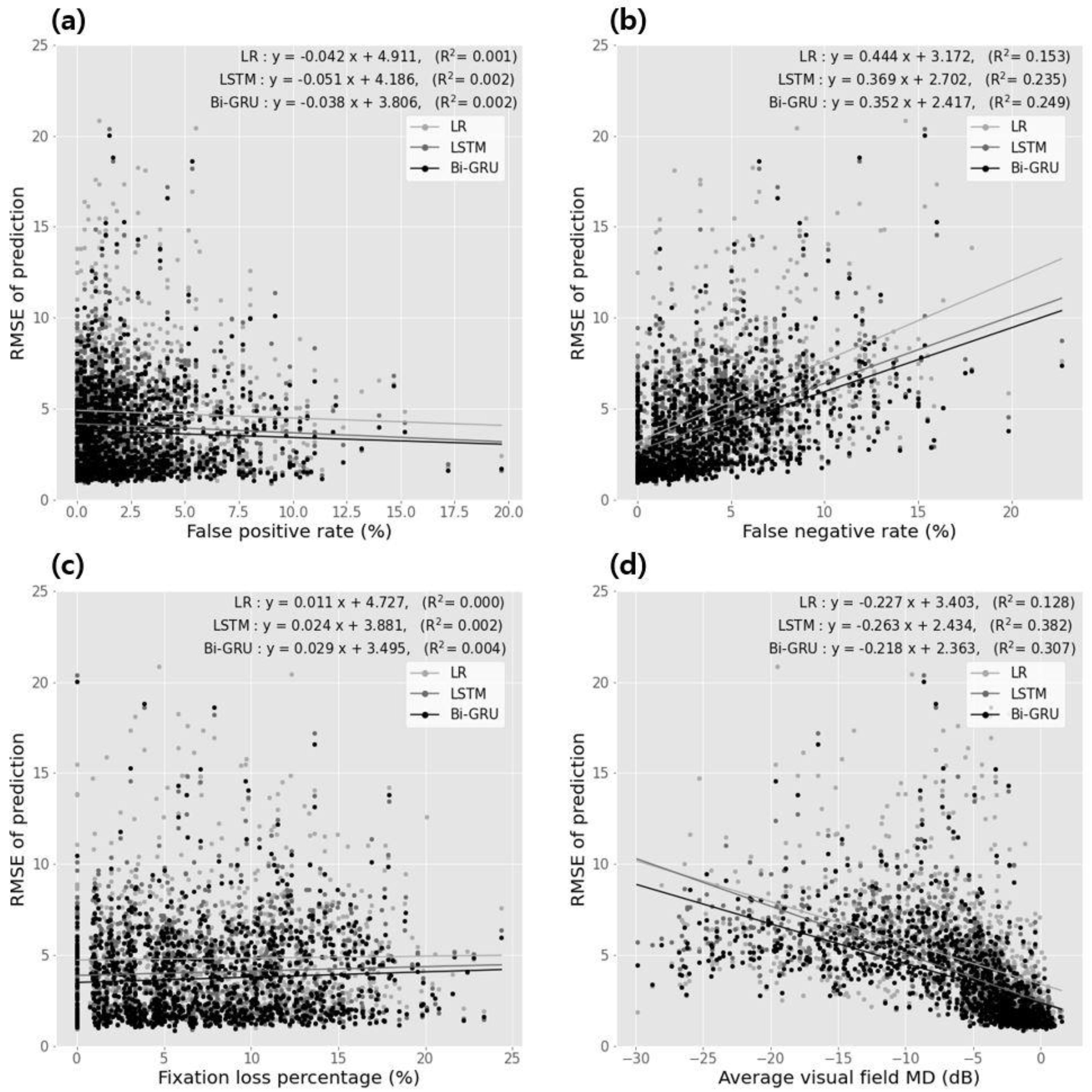
| Correlation Coefficients | Linear Regression Analysis | |||||
|---|---|---|---|---|---|---|
| Spearman’s rho | p-Value | Slope | Intercept | p-Value | ||
| classification error vs. false positive rate | ||||||
| Regression method | −0.024 | 0.344 | −0.042 | 4.911 | 0.001 | 0.329 |
| HMM | −0.043 | 0.040 | −0.041 | 4.184 | 0.002 | 0.048 |
| R-CNN | −0.042 | 0.134 | −0.038 | 3.804 | 0.002 | 0.141 |
| classification error vs. false negative rate | ||||||
| regression method | 0.444 | <0.001 | 0.444 | 3.142 | 0.143 | <0.001 |
| HMM | 0.443 | <0.001 | 0.349 | 2.402 | 0.234 | <0.001 |
| R-CNN | 0.448 | <0.001 | 0.342 | 2.414 | 0.249 | <0.001 |
| classification error vs. fixation loss percentage | ||||||
| regression method | 0.083 | 0.003 | 0.011 | 4.424 | <0.001 | 0.424 |
| HMM | 0.041 | 0.029 | 0.024 | 3.881 | 0.002 | 0.101 |
| R-CNN | 0.044 | 0.004 | 0.029 | 3.494 | 0.004 | 0.032 |
| classification error vs. average visual field average deviation | ||||||
| regression method | −0.441 | <0.001 | −0.224 | 3.403 | 0.128 | <0.001 |
| HMM | −0.443 | <0.001 | −0.243 | 2.434 | 0.382 | <0.001 |
| R-CNN | −0.444 | <0.001 | −0.218 | 2.343 | 0.304 | <0.001 |
Publisher’s Note: MDPI stays neutral with regard to jurisdictional claims in published maps and institutional affiliations. |
© 2022 by the author. Licensee MDPI, Basel, Switzerland. This article is an open access article distributed under the terms and conditions of the Creative Commons Attribution (CC BY) license (https://creativecommons.org/licenses/by/4.0/).
Share and Cite
Hosni Mahmoud, H.A. RETRACTED: Diabetic Retinopathy Progression Prediction Using a Deep Learning Model. Axioms 2022, 11, 614. https://doi.org/10.3390/axioms11110614
Hosni Mahmoud HA. RETRACTED: Diabetic Retinopathy Progression Prediction Using a Deep Learning Model. Axioms. 2022; 11(11):614. https://doi.org/10.3390/axioms11110614
Chicago/Turabian StyleHosni Mahmoud, Hanan A. 2022. "RETRACTED: Diabetic Retinopathy Progression Prediction Using a Deep Learning Model" Axioms 11, no. 11: 614. https://doi.org/10.3390/axioms11110614
APA StyleHosni Mahmoud, H. A. (2022). RETRACTED: Diabetic Retinopathy Progression Prediction Using a Deep Learning Model. Axioms, 11(11), 614. https://doi.org/10.3390/axioms11110614