1. Introduction
During the last few decades, the semi-parametric Cox proportional hazard (PH) model has dominated survival data analysis. While Cox’s original research paper discussed extensions to remove the assumption of PH [
1], much work has been carried out to improve the flexibility of survival regression frameworks by using tractable functions for both the baseline and the inclusion of covariates, primarily using probability distributions, splines, or fractional polynomials [
2].
As a matter of fact, the hazard rate and odds functions are two probabilistic functions with significant practical value in survival analysis. They both take into account the hazard rate or odds for a reference level associated with a link function of the covariates, which is often represented by a log-linear or a multiplicative term . Each covariate’s associated parameters are represented by the vector . Given a design matrix X and a subject , the vector represents covariate values. The subject i with all of its covariate values equal to zero represents the reference level.
So, based upon the type of probabilistic function utilized as a baseline function, the survival regression model classes can be divided into two primary groups: hazard-based regression models and odds-based regression models. However, the general design of those models did not change; the hazard or odds function was expressed as a baseline function multiplied by the link function of the covariates to either the baseline function, the time scale, or both of them.
Because of the most well-known Cox PH model, hazard-based regression models are the most prevalent survival regression model classes in the field of survival analysis. Consequently, there are four widely used hazard-based regression models: proportional hazard (PH) [
1,
3], accelerated hazard (AH) [
4], accelerated failure time (AFT) [
5,
6], and general hazard (GH) [
7,
8,
9,
10]. The odds-based regression models, which are created using a probabilistic function that has recently received more attention and is known as the odds function, are another family of survival regression model classes. Although the odds function is used in epidemiological case-control research, the proportional odds (PO) model class that was presented by Bennet [
11] is the first to apply it in survival models. AFT model is another odds-based regression model [
3]. As a result, just like hazard-based regression models, odds-based models are divided into four primary categories: PO [
11], accelerated odds (AO), AFT [
5], and general odds (GO) models.
There are other survival regression models as well, which combine hazard-based and odds-based regression models and are built by taking into account both hazard rate and odds functions. For instance, Yang and Prentice [
12] developed the Yang-Prentice model, a semi-parametric survival regression model that can include crossover survival curves. In order to describe survival data with crossed survival curves, Demarqui and Mayrink [
13] modified the Yang-Prentice (YP) model using a piecewise exponential baseline distribution. Both the PH and PO models are included as sub-models in the YP model. A generalized odds-rate hazards model was developed by Banerjee et al. [
14] and includes the PH, PO, and AFT models as special cases.
For censored lifetime data, Royston and Parmar [
15] presented a flexible parametric model based on the PH and PO models. On the other hand, Huang et al. [
16] also introduced a general class of regression model called the PH-PO model, which includes PH and PO models as sub-models. Huang and Jiang [
17] proposed an extension of the PH-PO model into a more generalized model that takes into account time scale changing effects and time varying coefficient effects. A semi-parametric super model containing six popular survival regression models, including the PH, PO, AFT, AH, YP, and GH models, was recently proposed by Zhang et al. [
18]. Davis [
19] has recommended the development of further new families that combine hazard-based and odds-based regression models. For additional details, please see [
20].
The absence of a general class of odds-based and hazard-based regression models that encompasses all hazard-based and odds-based regression frameworks is an issue that needs to be addressed. Each of the hazard-based and odds-based regression model classes mentioned above can capture different aspects of survival data. On the other hand, choosing which hazard-based or odds-based regression model is the most suitable and precise in reflecting the link between baseline (hazard or odds) and covariates, is an issue and an important research problem that must be addressed. To explicitly nest simpler models and to address the issue, we propose a novel, general, flexible, fully parametric class of hazard-based and odds-based regression framework named “Amoud class (AM)”.
In contrast, there are three categories of survival regression model classes: non-parametric, semi-parametric, and parametric models. Compared to non-parametric and semi-parametric methods, parametric models are more informative. They can be used to forecast survival times, hazard rates, as well as mean and median survival times in addition to computing relative effect estimates [
21]. They can also be used to plot covariate-adjusted survival curves and forecast absolute risk over time. Semi-parametric models lack the power of parametric models when the parametric form is incorrectly stated. Additionally, they are more effective, resulting in estimates with reduced standard errors and greater accuracy [
22,
23]. Furthermore, parametric techniques use full maximum likelihood to estimate parameters. Parametric model residuals often take the form of the discrepancy between what was observed and what was expected [
24].
Considering the discussion above, the current study proposes a fully parametric class of regression models that comprises formally nested special cases of the PH, PO, AH, AO, AFT, GH, and GO survival regression models. As a result, model selection among these models can be accomplished by conducting approximate likelihood ratio tests using the frequentist approach. To describe baseline hazard or baseline odds, a generalized log-logistic (GLL) distribution containing some of the most frequent parametric baseline distributions used in survival analysis, such as the log-logistic (LL), Bur-XII, exponential, and Weibull distributions, is employed. A right-censoring mechanism is considered, and the proposed model’s parameters are evaluated using maximum likelihood estimation and Bayesian estimation techniques. A real-world right-censored survival dataset with a crossing survival curve is utilized to demonstrate how the proposed AM class can be employed.
Hence, the novelty of this research paper is to introduce and investigate a novel, general, tractable, fully-parametric class of hazard-based and odds-based regression model for dealing with right-censored survival data with or without crossing survival curves. This is accomplished by assuming the GLL distribution in the proposed class to cope with the baseline distribution. To the author’s best knowledge, no one has ever contemplated employing the parametric AM class of parametric hazard-based and odds-based regression models in general, and with GLL baseline hazard in particular. This class is an extension of the most common hazard-based and odds-based regression frameworks in the literature. On the other hand, another area of interest that has yet to be addressed in the context of the AM class is the use of both the inferential procedures, Bayesian and frequentist approaches. As a result, the strategies are investigated utilizing the frequentist approach using the maximum likelihood estimation (MLE) method and the Bayesian approach using non-informative priors.
The structure of the article is as follows:
Section 2 presents a review of the hazard-based, and odds-based regression models in the context of survival, duration, and reliability analysis. The formulation of the AM class, its associated probabilistic functions, and sub-models of the class are discussed in
Section 3.
Section 4 describes the baseline distribution under examination in this study, as well as some of its special circumstances.
Section 5 presents the estimation of the proposed class parameters using both classical MLE and Bayesian estimation approaches.
Section 6 focuses on the model selection situations for both nested and non-nested models.
Section 7 shows a real-world, right-censored cancer dataset with crossing survival curves.
Section 8 finishes the study with a farewell address and recommendations for future research.
2. Recent Literature Review and State of Art
In this section, we review the studies completed in the framework of the hazard-based and odds-based regression models that are closely related to the proposed class in order to illustrate the state of scientific development in the context of current survival, duration, and reliability models.
2.1. Hazard-Based Regression Models
In general, survival datasets are highly skewed and can be censored for some subjects, possibly even the most. Standard linear regression models cannot fit them, and they also only allow for the interpretation of regression coefficients in terms of the mean of time. However, different models can be applied to survival data to generate different interpretations. Observed times’ functions rather than the observed times themselves are used for this. The hazard rate and the odds functions, in particular, are two probabilistic functions that are extremely important practically in survival analysis.
There are four major types of hazard-based regression models proposed in the literature to fit survival time data in medical investigations, namely, PH, AH, AFT, and GH models. These models can be used to analyze real-world data in domains other than medicine, such as economics, marketing, engineering, social science, criminology, and education. The modeling approach differs depending on the researcher’s event of interest; the general notion is to watch time until the event occurs; however, for some subjects, the event never occurs.
The formulation and construction of four hazard-based regression models are reviewed and discussed in this section. We define the alternative structures below using the hazard rate function (hrf), odds function, survival (complementary distribution) function (sf), and cumulative (or integrated) hazard function (chf) in relation to time t and a vector of covariates x. We suppose that the vector of covariates lacks an intercept to avoid concerns about identifiability. The unknown regression coefficients are represented by a vector .
2.1.1. PH Model
The semi-parametric PH model introduced by Cox [
1] is one of the most well-known hazard-based regression models in survival analysis. The hrf is multiplicatively affected by the impact of the covariates in this model. Different researchers have examined and analyzed studies relating to the parametric PH model utilizing various baseline distributions and inferential techniques. A parametric PH model, with an extended exponential geometric baseline distribution was developed and evaluated by Rezaei et al. [
25]. A parametric PH with GLL baseline distribution was also proposed by Khan and Khosa [
23]. A modified PH model and a reversed PH model employing the Marshall-Olkin baseline distribution were examined by Balakrishnan et al. [
26]. Muse et al. [
27] have investigated the Bayesian analysis of the PH model with a GLL baseline distribution.
The PH model’s hrf, odds, sf, and the chf can be stated as follows:
where
,
,
, and
are the baseline hazard rate, odds, survival and cumulative hazard functions.
2.1.2. AFT Model
The PH model is the most popular hazard-based regression model in survival analysis, but it can only be used in situations in which the PH assumption holds. An alternative to the PH model is the AFT model [
3,
5]. The AFT model is analogous to a hazard-based regression model in which covariates measured on an individual are assumed to act multiplicatively on the time-scale, influencing the rate at which the individual advances along the time axis. Numerous scholars have studied and discussed studies involving the parametric AFT model using various baseline hazards and statistical inference techniques. A parametric AFT model with an exponentiated Weibull baseline distribution was presented and analyzed by Khan [
22]. A parametric AFT with a log-exponential power baseline distribution was also proposed by Olosunde et al. [
28]. Ashraf-Ul-alam and Khan [
29] used a generalized Top-leone-Weibull baseline distribution to study a parametric AFT model. A parametric AFT model with a GLL baseline distribution was recently proposed by Muse et al. [
30].
The hrf, odds, sf, and chf of the AFT model are defined by:
2.1.3. AH Model
AFT and PH models have been widely applied to deal with lifetime data in different disciplines of knowledge. Despite being widely used, such hazard-based regression models are not suitable to handle survival data with crossing survival curves. Chen and Wang [
4] proposed a semi-parametric hazard-based regression model, named the AH model, allowing the analysis of crossing survival curves. In the context of a parametric AH model, different baseline hazards are available in the AHSurv package [
31].
The hrf, odds, sf, and chf of the AH model are defined by:
2.1.4. GH Model
Ciampi and Etazadi-Amoli [
7] introduced a general hazard (GH) regression model for testing the PH and the AFT hypothesis in the analysis of censored lifetime data with the presence of covariates. Then, Etazadi-Amoli and Ciampi [
8] extended their work by the application of the splines as a baseline function. It is worth to mention that the EHR model requires a careful selection of the knots and could easily lead to an overparametrized or non-identifiable model. On the other hand, Chen and Jewell [
10] introduced a general class of semi-parametric hazard-based regression models by following the same procedure as [
7] but just by adding the AH framework. The case of parametric GH structure in the context of relative survival framework was introduced by Rubio et al. [
2] and developed an R Package called GHSurv available in
https://github.com/FJRubio67/GHSurv (accessed on 5 October 2022) and HazReg package that contain several choices of the baseline hazards (
https://github.com/FJRubio67/HazReg, accessed on 5 October 2022). Recently, Muse et al. [
32] proposed the over survival framework for the GH model using both Bayesian and classical inferences. Consequently, Alvares and Rubio [
33] discussed the GH structure in the context of joint models for longitudinal and survival datasets. Finally, in the context of the a spatial survival models, Li et al. [
34] extended the GH model to spatial GH model. Recently, Rubio and Drikvandi [
35] modified the
structure into a mixed-effect general hazard (MEGH) model to account for cluster survival datasets.
The hrf, odds, sf, and chf of the GH model are expressed as follows:
where
and
denote the unknown regression parameters.
2.1.5. Special Cases of the GH Model
All of the hazard-based regression models listed above are incorporated into the GH model of hazard-based models as special cases. The GH model can be used to derive the PH, AH, and AFT models, according to the following proposition.
Proposition 1. Suppose is given by Equation (13). Then, we have the following results: 1. If , then giving the AFT model.
2. If , then giving the PH model.
3. If , then giving the AH model.
Proof of Proposition 1. The proof of Proposition 1 is straightforward. □
2.2. Odds-Based Regression Models
To fit survival time data in medical research, two primary types of odds-based regression models have been proposed in the literature: PO and AFT models. Two more innovative odds-based regression models proposed in this study are the accelerated odds and general odds models. In fields other than medicine, such as economics, marketing, engineering, social science, criminology, and education, these models can be utilized to examine actual data.
The odds function indicates how much more likely it is that a particular event will occur for a given period
t. As a result, the odds function is denoted by
, and its mathematical expression is given by the relationship between the cumulative distribution function and its complementary (sf):
where
, and
are the odds, cumulative distribution, survival and cumulative hazard functions respectively, and
is the vector of distributional parameters.
The associated derivative of the odds function is expressed as follows:
where
, and
represent the odds, hrf, and probability density function (pdf), respectively.
In this section, we review two odds-based regression models that have been explored in the literature along with their formulation. On the other hand, based on the author’s knowledge, we present two novel odds-based regression models that have never been used before in the literature. We define the alternative structures below with respect to time t and a vector of covariates x using the odds function , derivative of odds function , hrf , and sf . We assume that the covariate vector is free of an intercept to ease issues about identifiability. The vector is used to represent the unknown regression coefficients.
2.2.1. PO Model
The proportional odds (PO) model, originally introduced by Bennett [
11], is an odds-based regression model. According to Bennett [
11], the PO model is structurally similar to the PH model of Cox and may be used in similar situations. Although the PO model represents an attractive alternative to the PH model.
The odds function of this model is expressed as follows:
where
is the baseline odds function. The associated derivative of the odds function of the PO model is computed as follows:
where
is the baseline derivative odds function.
The hrf of the PO model is computed as follows:
In terms of the baseline hazard, the hrf, and sf can be expressed as follows using Equation (
18):
Now, we will put forth two new models that employ methods related to the hazard-based regression models. All of the odds-based regression models in this section will be generalized as well. The model formulation put forward by Chen and Wang [
4] served as inspiration for the initial proposed approach. Their model includes accelerated hazards, but we propose a model with accelerated odds. This is how our models differ from theirs. The model formulation proposed by Chen and Jewell [
10] served as the basis for the second proposed model. The PH, AH, and AFT models are included in their models as sub-models. In contrast to their model, ours includes the PO, AFT, and AO models as sub-models. The general odds model is the name of this model. The odds-based regression models with different baseline distributions are available in the AmoudSurv Package [
36].
2.2.2. Accelerated Forms
The second parametric method of taking into account the effect of covariates, known as the accelerated form, presupposes that the covariates directly rescale time. Accelerated effects of covariates come in two varieties: Two examples of this are the:
- i.
Accelerated failure time (AFT) model; and
- ii.
Accelerated odds model.
The accelerated types of the odds-based regression models can be formulated in two different ways, the first of which is similar to the AFT model. The AFT model is the only parametric survival regression framework that belongs to both the hazard-based and odds-based regression models, and both the continuous probability distributions that are closed under the hazard-based regression models and those closed under the odds-based regression models are consistent with the AFT model. For instance, the Weibull and LL distributions. We will explore these distributions in
Section 4 of this study. Based on what the authors know, accelerated odds (AO) model is a new survival regression model that has never been used previously.
The formulation one belongs to the AFT framework and can be expressed as follows:
The associated derivative of the odds function of the AFT model is computed as follows:
The hrf and sf are expressed as follows:
This model, as one can see after its derivation and simplification, is similar to the AFT model. As a result, we can remark that the AFT model is the only one of the survival regression models that holds true for both hazard-based and odds-based regression models.
2.2.3. Accelerated Odds Model
A novel parametric odds-based regression model that can incorporate censored lifetime datasets with crossing survival curves is introduced here and named the “accelerated odds
” model. This model is formulated using the odds function, and by using the same procedure as for the AH model, we obtained the following parametric odds-based regression model that is a new one and has not been featured in the literature so far:
The associated derivative of the odds function of the AO model is computed as follows:
The hrf and sf are expressed as follows:
2.2.4. General Odds Model
Another novel general survival regression model, termed the “general odds (GO)” model, is introduced here and consists of three odds-based regression models as special cases, namely: PO, AFT, and AO models. The odds function of this model can be computed as follows:
The associated derivative of the odds function of the GO model corresponding to the odds function in Equation (
32) is computed as follows:
The hrf and sf of the GO model corresponding to Equation (
32) are expressed as follows:
In terms of the odds function, the sf in Equation (
35) of the GO model can be computed as follows:
2.2.5. Special Cases of the GO Model
All of the odds-based regression models listed above are incorporated into the GO model of odds-based models as special cases. The GO model can be used to derive the PO, AO, and AFT models, according to the following proposition:
Proposition 2. Suppose is given by Equation (33). Then, we have the following results: 1. If , then giving the AFT model.
2. If , then giving the PO model.
3. If , then giving the AO model.
Proof of Proposition 2. The proof of Proposition 2 is straightforward. □
3. The Proposed Class
3.1. Why AM Class of Hazard-Based and Odds-Based Regression Models?
All of the hazard-based and odds-based regression models discussed in the preceding
Section 2 can model different aspects of time-to-event data. However, determining which model is the most accurate and precise in revealing the correlation between explanatory variables and the baseline hazard (or the baseline odds) is a challenging issue and a significant research question that must be addressed.
In real life, we must decide between hazard-based regression models and odds-based regression models when provided with a dataset. A popular technique would be to fit one model to each of them, and then test the model to determine where it falls well short. However, the possibility of verifying the model assumptions may be constrained due to the finite sample size and other data characteristics. Additionally, if the right time-dependent covariates are taken into account, both the hazard-based models, such as the PH, AFT, AH, and GH models, and the odds-based models, such as the PO, AO, AFT, and GO models, may be able to fit the data relatively well.
Another issue with time-to-event data is that lifetimes can be censored in a variety of ways, including left, right, interval, double, and middle censoring, as well as survival data with crossover survival or hazard curves. Furthermore, a general class containing all of the preceding eight hazard-based and odds-based regression models is required. As a result, it is difficult to address all of the aforementioned open topics using both frequentist and Bayesian methods.
To address the aforementioned problems and to fill the gap, we introduce the AM class of hazard-based and odds-based survival regression models, a unique, novel, tractable, universal, parametric class of survival regression models that encompasses all hazard-based and odds-based regression models to help applied statisticians to decide which model to fit in a given censored survival dataset. We estimate the model parameters using both frequentist and Bayesian approaches, and we evaluate the proposed model’s nested structure using a likelihood ratio test.
In this section, we introduce the new survival regression model, its main probabilistic functions, and some special cases.
3.2. Model Formulation
Let
T be a non-negative random variable that represents the length of time until an event of interest occurs. As already sketched, a universal class for hazard-based and odds-based regression models called the “Amoud Class (AM)” has the following closed form in order to accommodate survival data with or without the crossover of the hazard and survival curves:
where
is the baseline odds function. This generality is attained using a structure resembling the general class of hazard-based regression models, with the addition that the baseline odds function is multiplied to a link function (i.e., log-linear function) for the covariates.
The sf for the AM model corresponding to the odds function in Equation (
37) is expressed as follows:
The hrf for the AM model corresponding to Equation (
37) is computed as follows:
3.3. Probabilistic Functions for the Amoud Class Model
In terms of odds function, the sf for the AM model in Equation (
38) can be expressed as follows:
The derivative of the odds function for the AM model is expressed as follows:
The cumulative distribution function (cdf) for the SM model is computed as follows:
where the baseline hazard, odds, survival, cumulative distribution, and the derivative of the odds functions are
(.),
,
,
, and
, respectively.
3.4. Special Sub-Models of the Proposed Class
All of the hazard-based and odds-based regression models listed above are incorporated into the AM Class of hazard-based and odds-based survival models as special cases. The AM class can be used to derive the PH, PO, AH, AO, AFT, GH, and GO models, according to the following proposition:
Proposition 3. Suppose is given by Equation (37). Then, we have the following results: 1. If , then , giving the GH model.
2. If , then , which is the GO model.
3. If , then , giving the AFT model.
4. If , then , which is the PO model.
5. If , then , giving the PH model.
6. If , then , which is the AO model.
7. If , then , giving the AH model.
Proof of Proposition 3. The proof of Proposition 3 is straightforward. □
Figure 1 illustrates the relationship between the proposed AM class and its sub-models including the GH, GO, AFT, AO, AH, PO, and PH models.
7. Practical Illustrations
A clinical trial right-censored oncology dataset is examined in this section to demonstrate the applicability and tractability of the proposed models, including the fully-parametric AM class, GO, and AO models with three different baseline distributions, including Weibull, LL, and GLL baseline distributions in modelling right-censored survival data with crossing survival curves. We compared the proposed AM class with its sub-models that contain both hazard-based regression models, including PH, AH, AFT, and GH models, and the odds-based regression models, including PO, AO, AFT, and GO models, using both the MLE frequentist and Bayesian approaches using noninformative priors. The class and its sub-models were compared using different information criteria, including the classical ones (AIC, BIC, BCAIC, CAIC, and HQIC), Bayesian model selection (WAIC, and LOOIC), and checking the nested structure of the AM class using the LRT test.
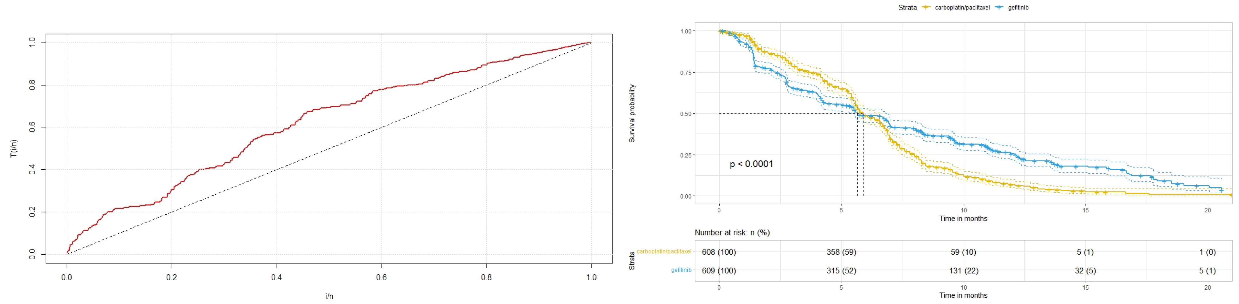
7.1. IPASS Clinical Trial Data Set
In order to show the applicability of the proposed models, we re-analyzed a large dataset from a randomized clinical trial called IPASS for this study. In a randomized controlled trial, gefitinib vs. carboplatin-paclitaxel was compared for progression-free survival in patients with advanced pulmonary adenocarcinoma. An unadjusted PH model was used to examine the main outcome. Despite the implicit violation of the PH model assumption represented by the crossing of the two survival curves, the study’s findings were published using this model [
51].
Argyropoulos and Unruh [
52] reconstructed and re-published the IPASS dataset, and it is now freely available in an AHSurv R package [
31].The features stated in the references are all still there in this reconstructed dataset, which is also accessible to the clinical trial’s results. The months of March 2006 through April 2008 are covered by the database. The main objective of the trial is to evaluate the effects of gefitinib versus carboplatin/paclitaxel doublet chemotherapy on progression-free survival (in months) in a subset of patients with non-small-cell lung cancer (NSCLC). According to the trial’s design,
previously untreated individuals in East Asia with advanced lung adenocarcinoma and who were non-smokers or previous light smokers were randomly assigned to either carboplatin + paclitaxel (608 patients) or gefitinib (608 patients) (609 patients). The observations show 965 occurrences of the event of interest (79.3 percent), with 449 (73.7 percent) relating to patients receiving gefitinib and 516 (84.9 percent) related to patients receiving carboplatin+paclitaxel.
The primary goal of this section is to appropriately assess the rebuilt IPASS data and estimate the regression coefficients using the proposed fully-parametric AM class provided in
Section 3. For the proposed model, we evaluate both the maximum likelihood and the Bayesian estimating approaches to achieve this goal.
We fit all hazard-based and odds-based regression models as well as the general proposed AM class using three different baseline distributions, namely Weibull, LL, and GLL distributions, letting
(treatment = chemotherapy), which equals 1 if the treatment involves gefitinib and 0 if the treatment involves carboplatin/paclitaxel.
Table 2,
Table 3 and
Table 4 provide a summary of the numerical results.
Figure 2 displays the total time on test (TTT) plot for the survival time and the survival curves of the two types of drugs where crossing between the curves can be seen, which confirms the efficacy of the proposed novel models in this study, including the AM, GO, and AO models, plus some other existing models in the literature, including the GH, and AH models, and that it is appropriate for the analysis of survival data with crossover survival curves.
The parameters and related standard errors from the various hazard- and odds-based regression models employing the Weibull baseline distribution and five different information criterion estimations are shown in
Table 2. The TTT plot in
Figure 2 shows that the data’s increasing hazard rate points to the theoretical use of the Weibull baseline distribution. According to the findings in
Table 2 and
Figure 3, the W-AM class has the lowest values for each information criterion when compared to all other competing regression models, demonstrating its superiority over other hazard-based and odds-based regression models. Another crucial aspect that restricts the use of the Weibull baseline distribution is the fact that all hazard-based regression models yield the same result, which is a weakness of the Weibull baseline distribution.
All hazard-based regression models, including the AH, PH, AFT, and GH models, produce the same findings when compared to the Weibull baseline as illustrated in
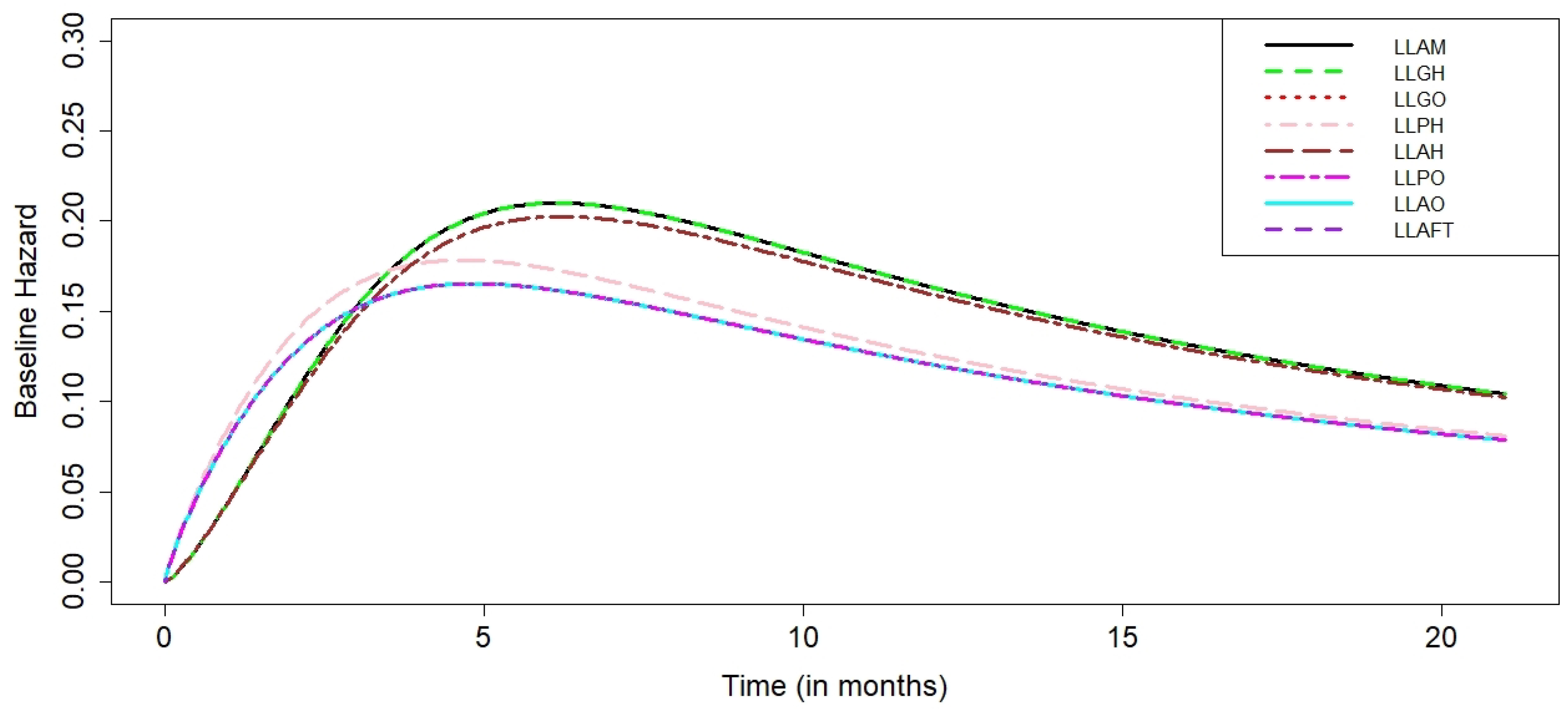
Table 2. The LL baseline distribution was used to fit and compare all of the regression models after we looked at an alternate baseline distribution. Using the LL baseline distribution and five different information criteria,
Table 3 provides estimates of the parameters and related standard errors from the various hazard-based and odds-based regression models. According to the AIC values in
Table 3, there is no clear preference for one model over the other. The fact that all odds-based regression models yield the same result is a significant factor that restricts the applicability of the LL baseline distribution.
When the Weibull distribution is used as the baseline distribution, all hazard-based regression models exhibit coincidence as shown in
Table 2. On the other hand, when the baseline distribution is an LL distribution, all odds-based regression models exhibit coincidence as illustrated in
Table 3, and
Figure 4.
These two points recommend looking for and utilizing a modified baseline distribution, which can provide us with various results for all survival regression models, regardless of whether they are hazard-based, odds-based, or a combination of both. We used the GLL baseline distribution, where a sub-model of the Weibull distribution that yields different results for all the regression models taken into consideration in this study, to close the gap and compare the seven different hazard-based and odds-based regression models that are currently in use.
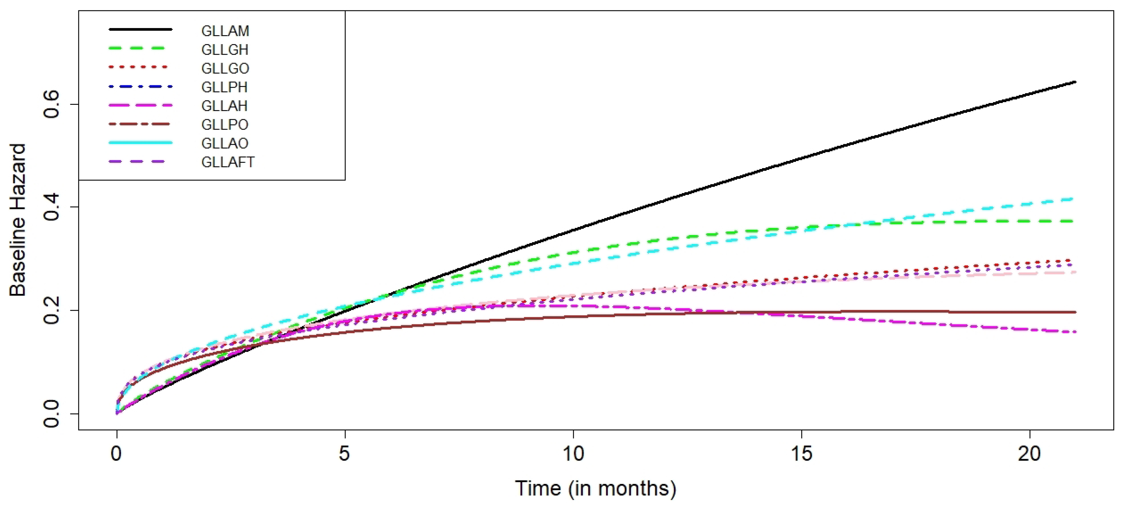
For the proposed AM class and seven different hazard- and odds-based regression models with GLL baseline distribution, the parameter estimates and their associated standard errors are shown in
Table 4. We see that for the eight competing models, the estimates of the baseline distribution parameters and their standard errors are quite similar and within a reasonable range. The GLL-AM model appears to be preferred above the other competing models and provided the best-fitting model, according to the values of the five distinct information criteria. The results also showed that the GH and GO models are preferred over their sub-models. Finally, the results indicate that the only basic survival regression models that can be used to model and analyze survival data with crossing survival curves are the AH and AO models.
The GLL-AM regression model is the best model compared to the others, according to the LRT results in
Table 5. The previously stated result is supported by the plots of the estimated hazards in
Figure 5.
According to the LRT results in
Table 6, the GLL-GH regression model is the most effective of the alternatives hazard-based regression models.
According to the LRT results in
Table 7, the GLL-GO regression model is the most effective of the alternatives odds-based regression models.
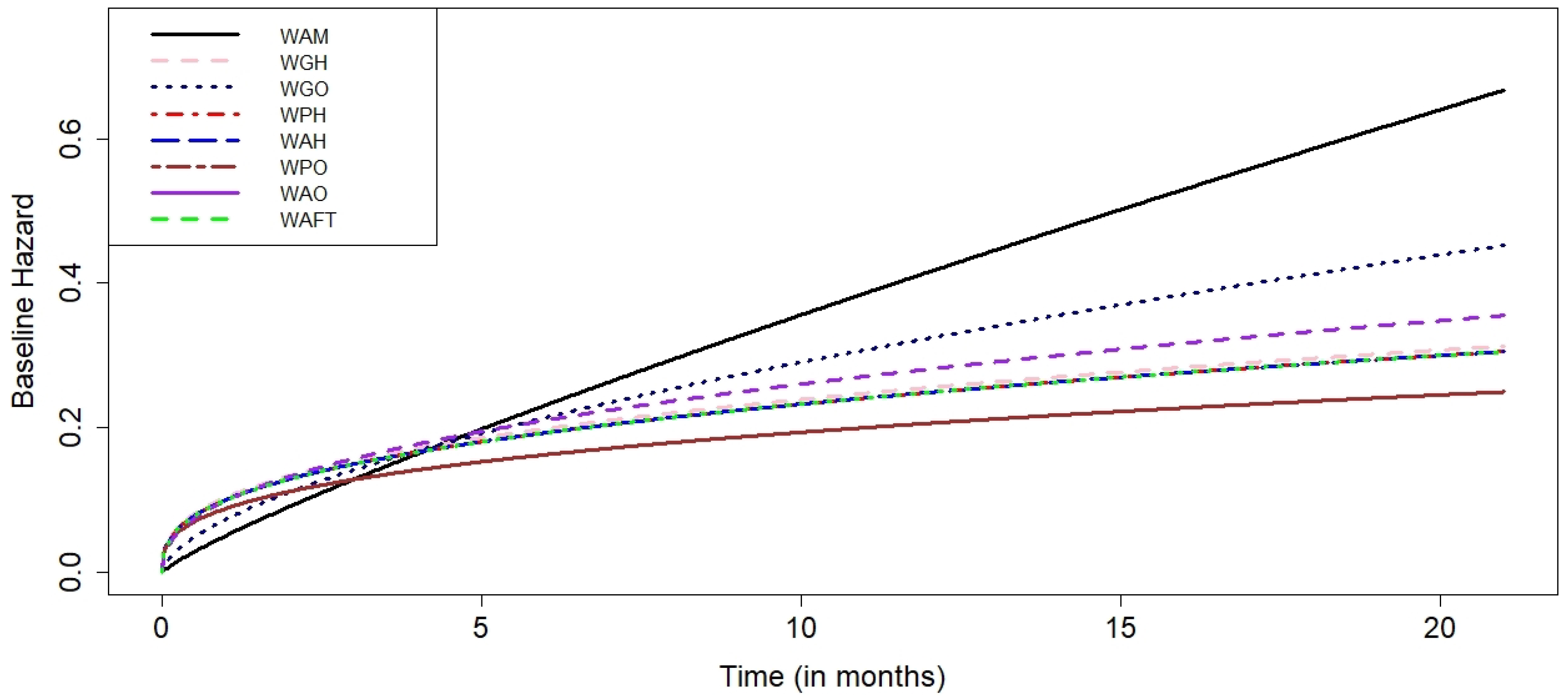
The W-AM model is the best model among the others, according to the hazard plots of the estimated hazard rates in
Figure 3, while other hazard-based models with the Weibull baseline distribution fitted similarly and there was no more difference at all. According to the plots in
Figure 4, there is no model that is preferred over the others when the baseline distribution is the LL distribution, and there is no difference between any of the odds-based regression models that were fitted. Finally, as illustrated in
Figure 5, the GLL-AM model is the superior compared to the other competitive models.
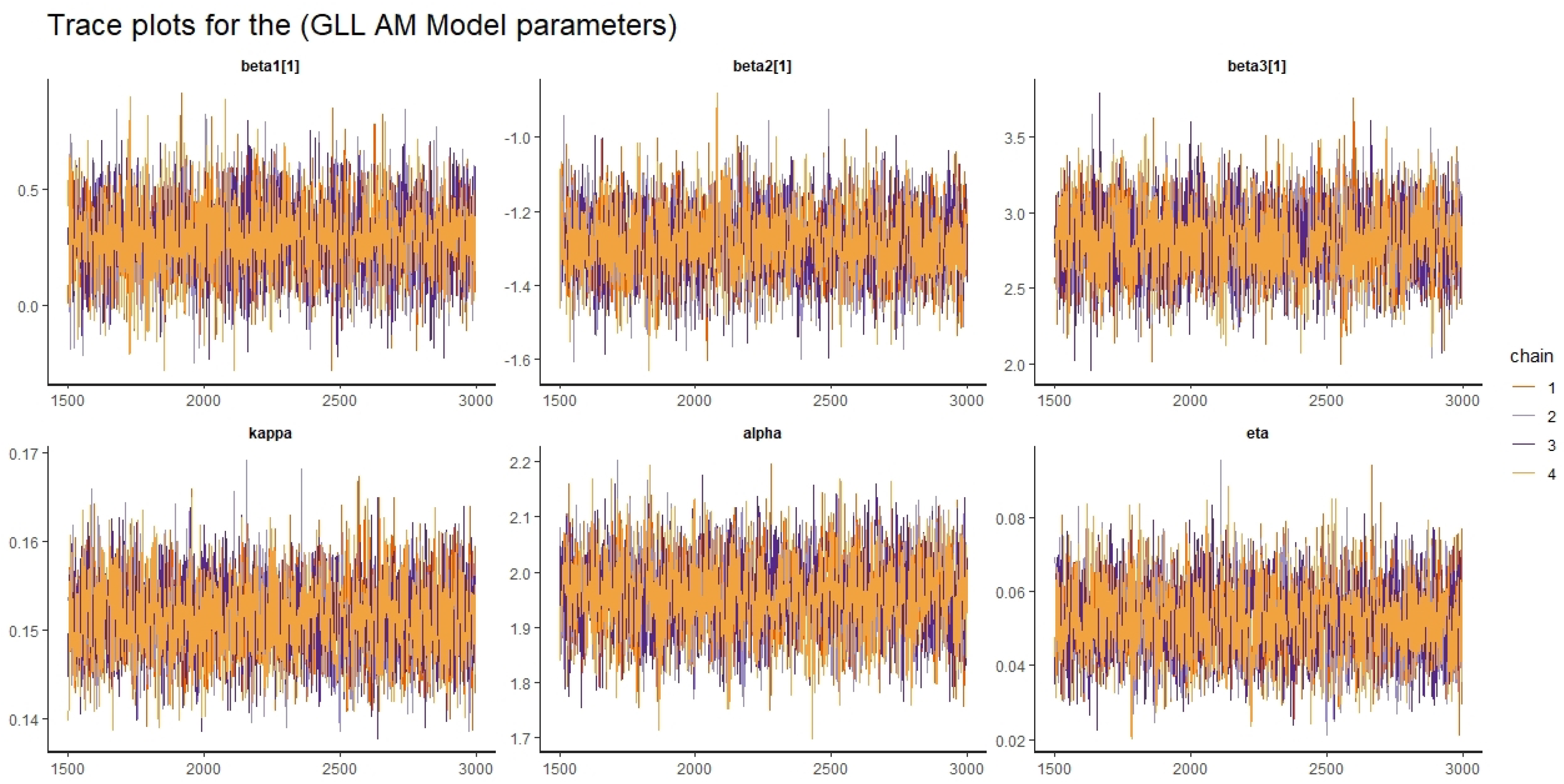
7.2. Bayesian Analysis
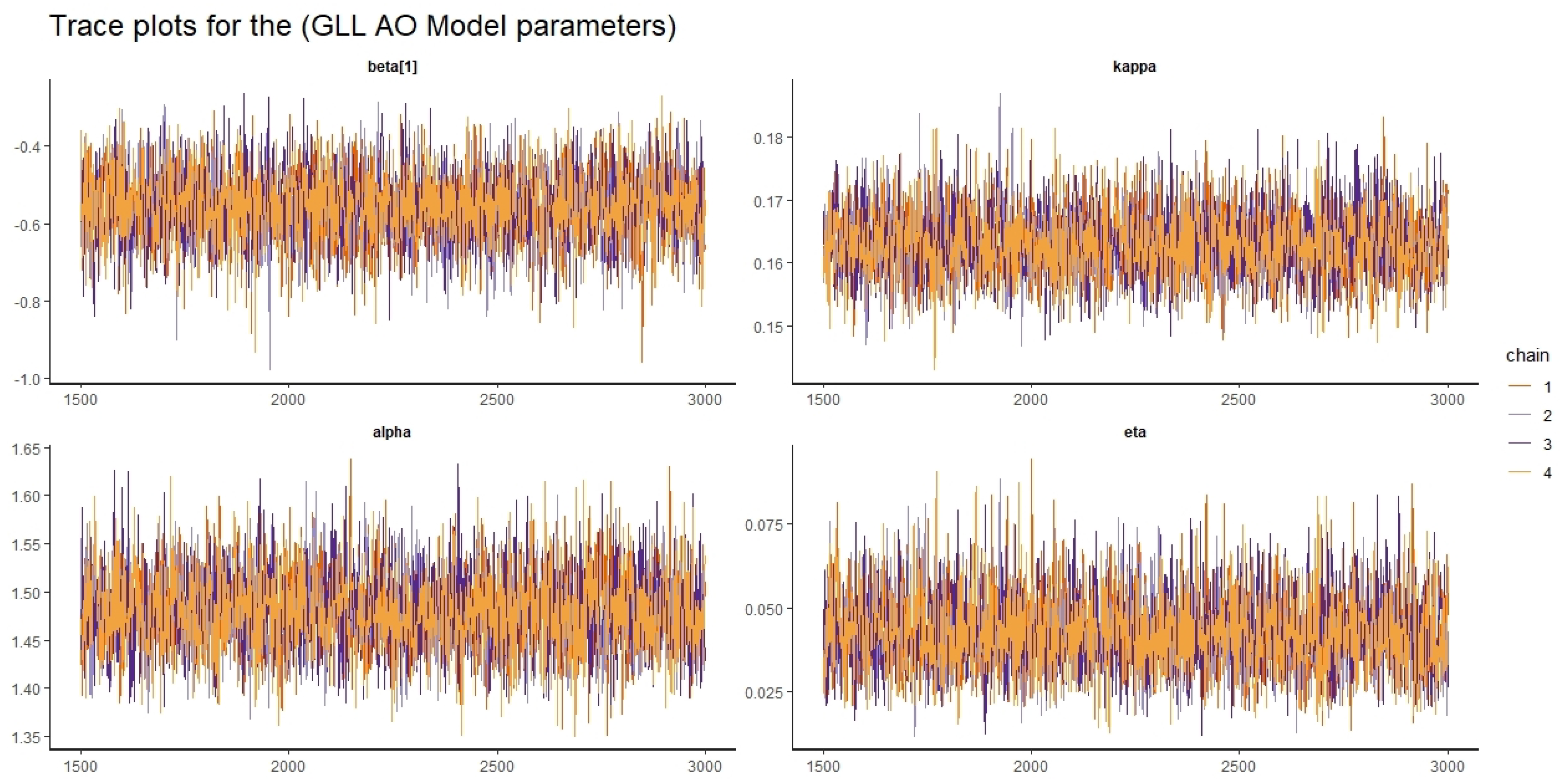
We performed all Bayesian inferential procedures resulting from the combination of the aforementioned general baseline distribution specifications with various prior scenarios in baseline parameters, as well as regression coefficients related to explanatory variables. Using the Rstan package in R [
53], the joint posterior distribution for each model was approximated. We performed four parallel chains with 3000 iterations and a burn-in of 1000 for each estimated model. To lessen autocorrelation in the sample, chains were also trimmed by storing after every fifth iteration. With a prospective scale reduction factor close to 1 and an actual number of separate simulation draws of more than 400, convergence to the joint posterior distribution was assured [
29,
54].
The posterior distribution’s numerical summary characteristics are summarized in
Table 8. According to the summary results, the McMC algorithm has converged to the joint posterior distribution because the potential scale reduction factor
is 1, the effective sample size
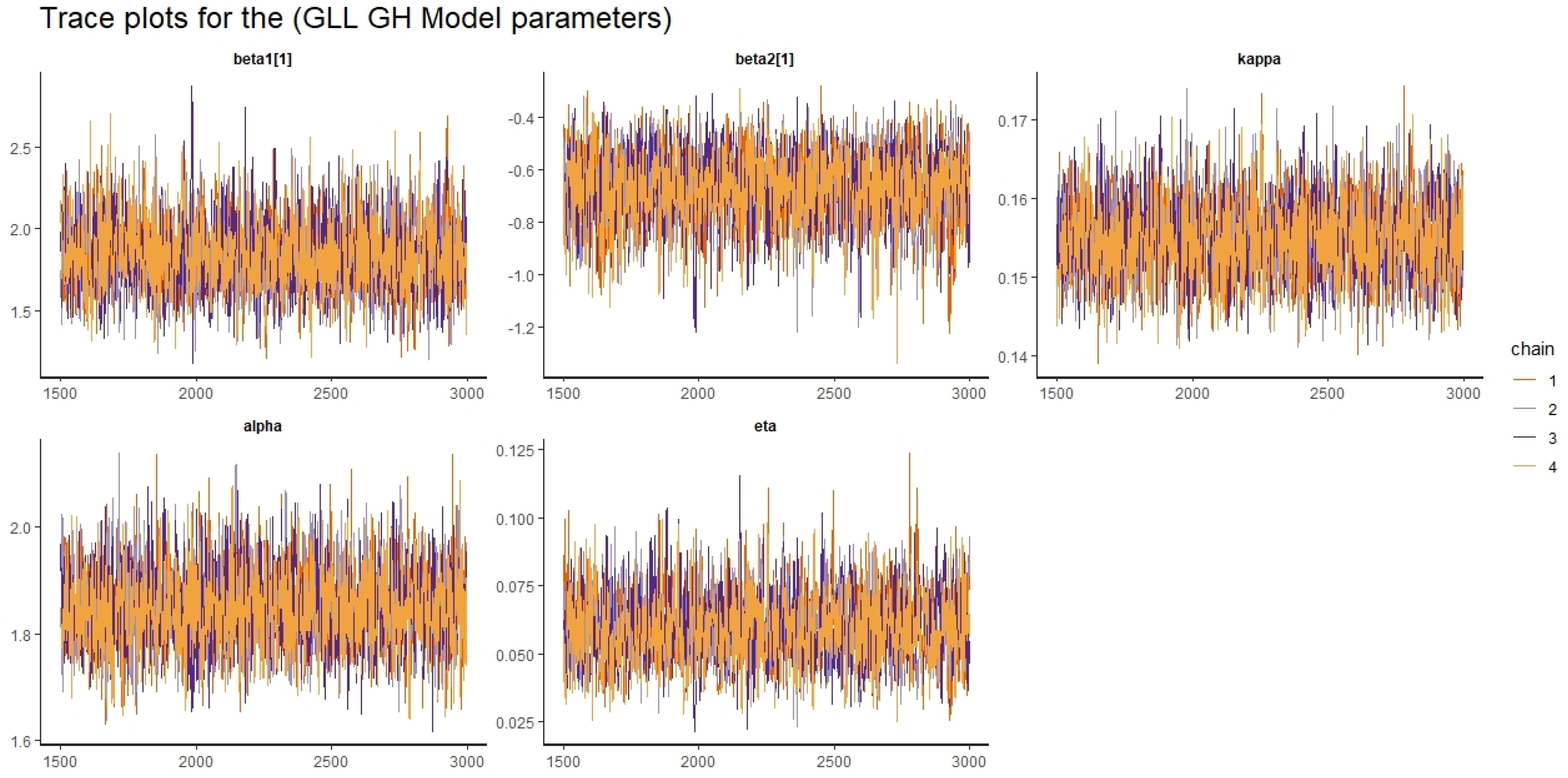
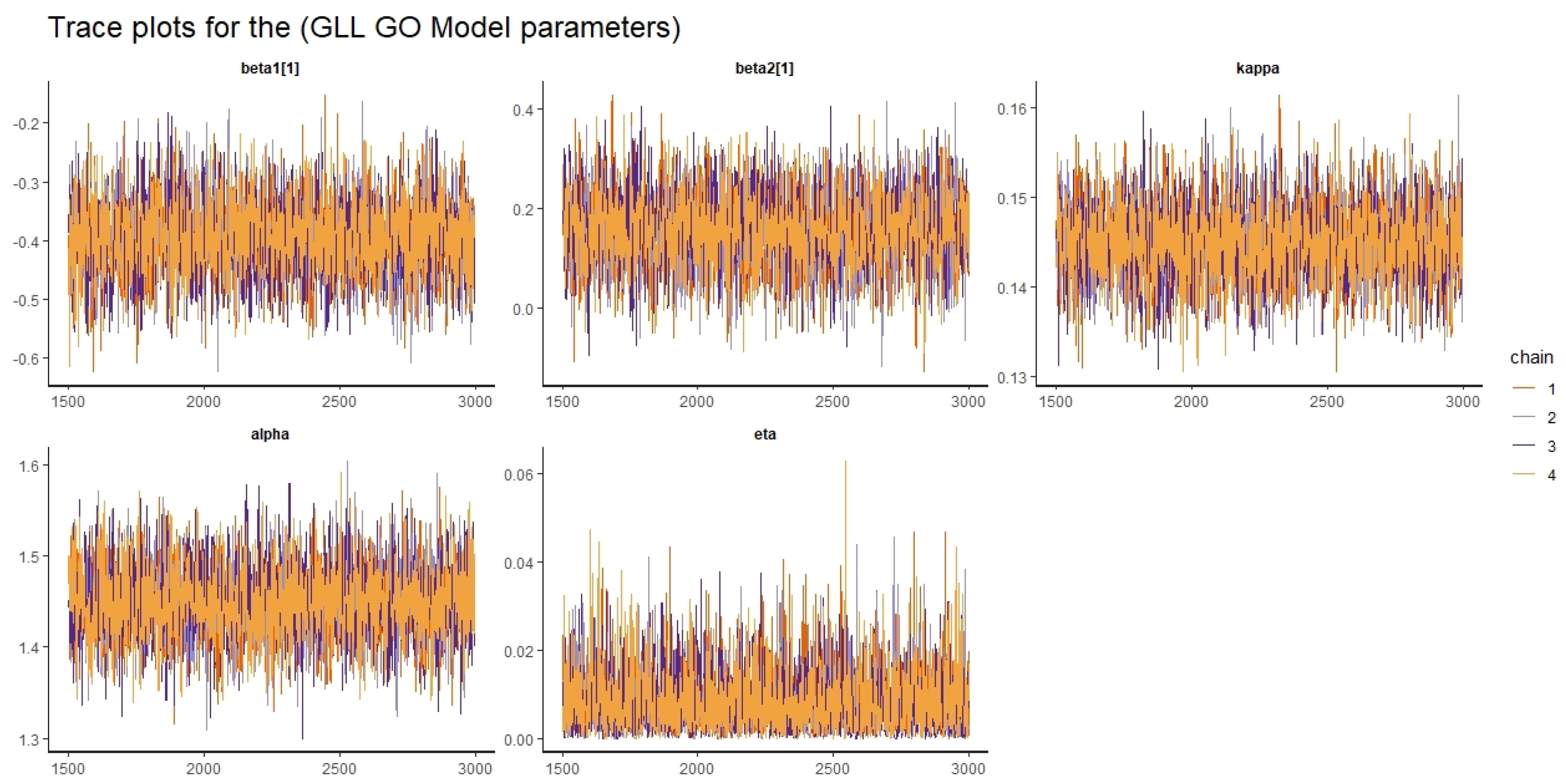
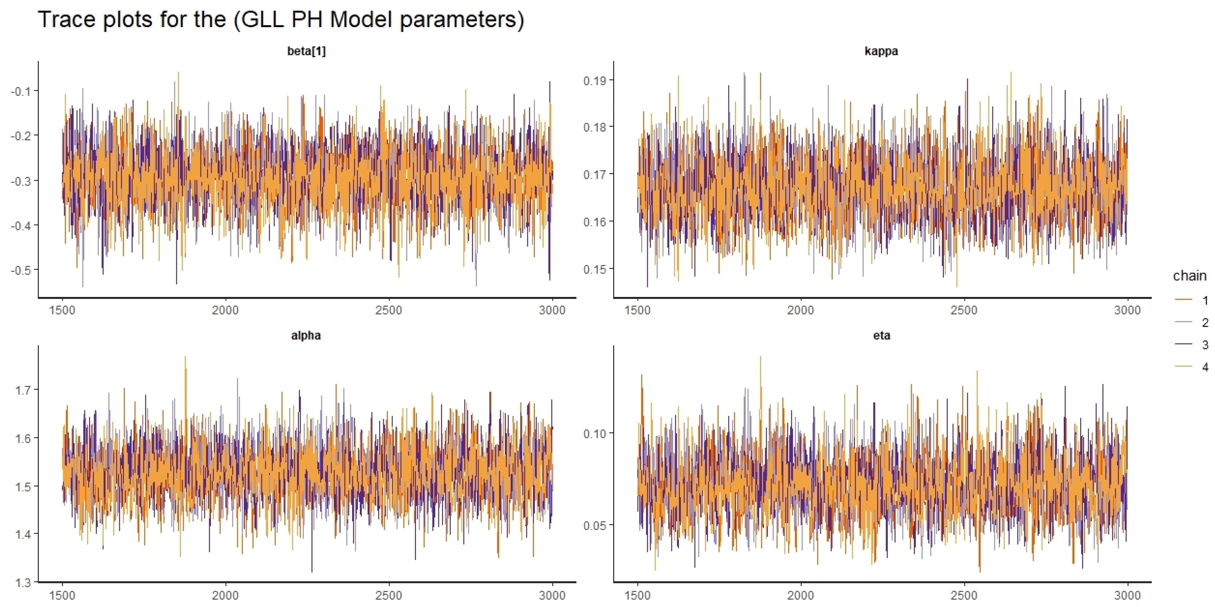
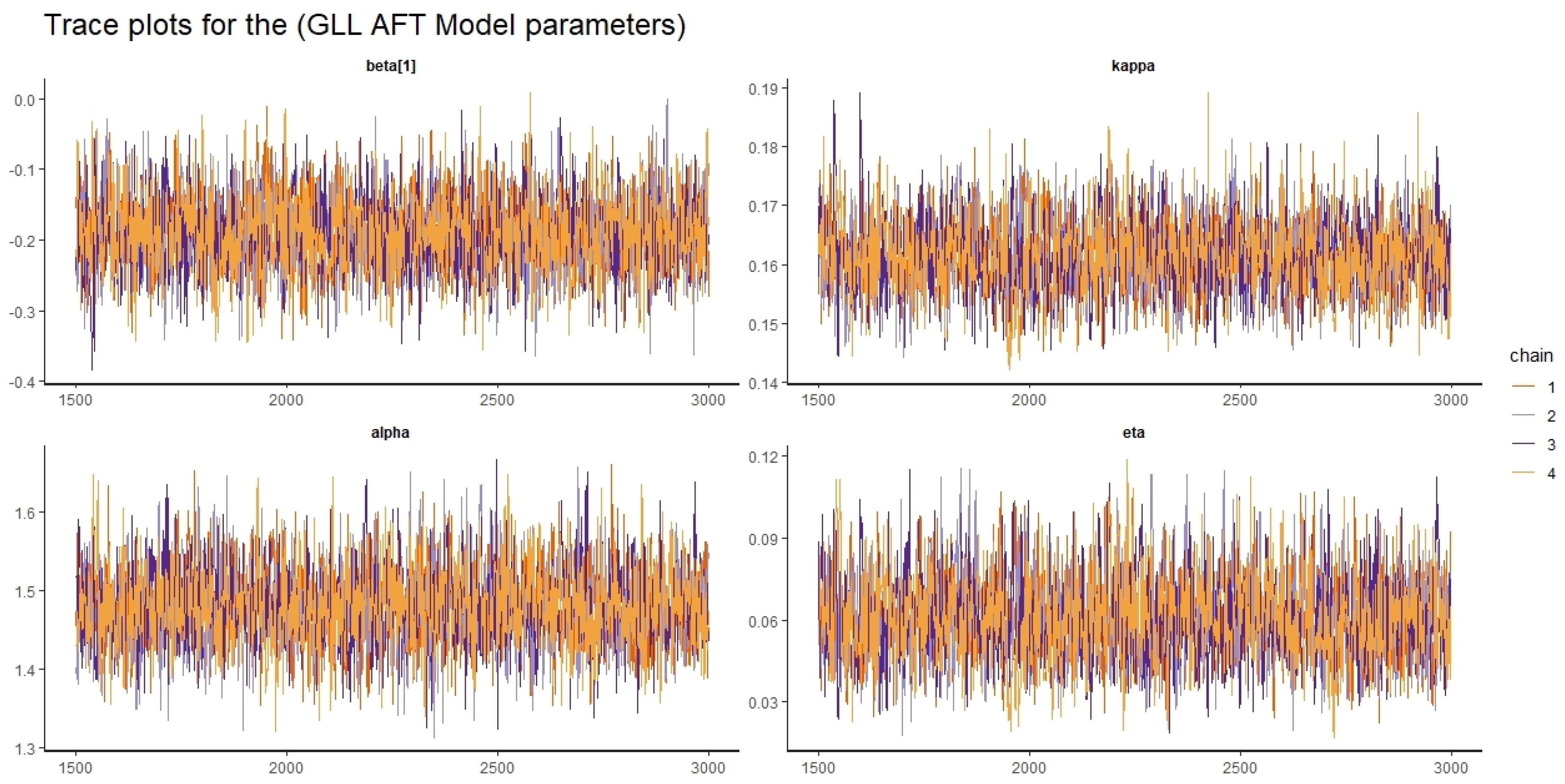
is greater than 400, and the Monte Carlo standard error (SE) is less than 5 percent of the posterior standard deviations (SD) for all of the parameters. For visually examining convergence, use trace graphs. The trace plots in
Figure 6,
Figure 7,
Figure 8,
Figure 9,
Figure 10,
Figure 11,
Figure 12 and
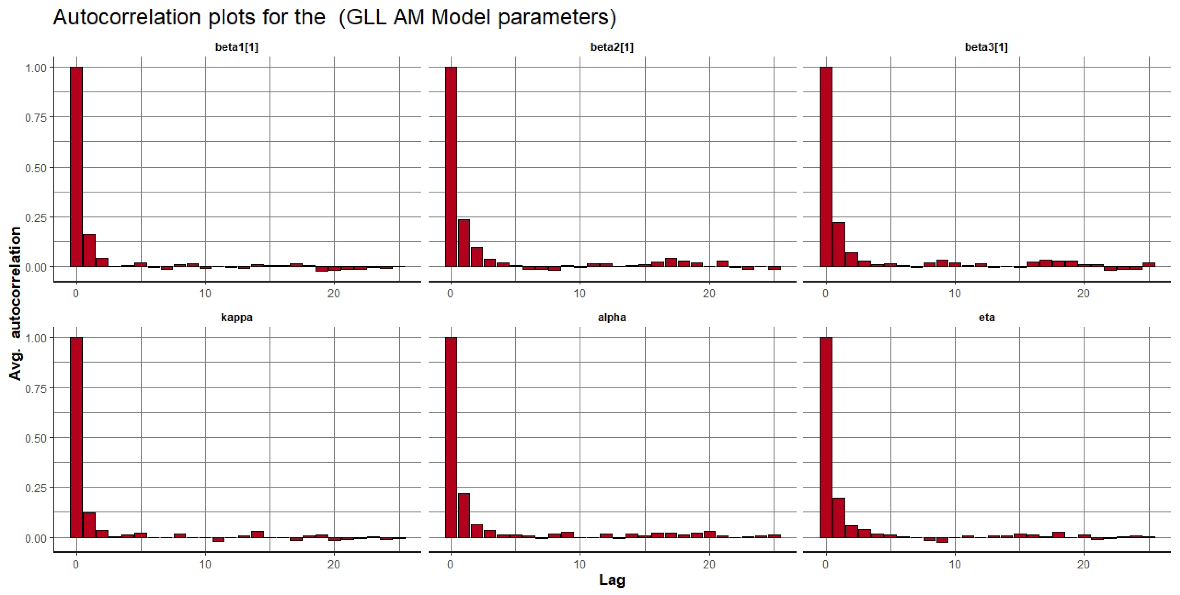
Figure 13 demonstrate a stationary pattern fluctuating inside a band, demonstrating convergence of the McMC algorithm. For the proposed AM class, density and autocorrelation graphs are also employed in
Figure 14 and
Figure 15, respectively, and both show that the McMC algorithm has converged.
Table 9 displays the computed models’ WAIC and LOOIC values. In comparison to the other fitted models, including the GLL-AH, GLL-AO, GLL-PO, GLL-AFT, GLL-GH, GLL-GO, and GLL-PH models, the GLL-AM model performs better based on the WAIC and LOOIC values. The worst performance is displayed by the most popular survival regression models, such as the PH, PO, and AFT models. This proves that, despite their frequent application, these models are not appropriate for handling survival data with crossing survival curves.
8. Conclusions
We investigated a novel, general, flexible, fully parametric class for hazard-based and odds-based regression models, named the AM class, with a GLL baseline distribution that can incorporate the basic shapes of the failure rate and contains, as specific cases, the main survival regression models of interest in time-to-event analysis: PO, PH, AO, AH, AFT, GO, and GH models. However, the AH, AO, and GO models’ restricted utility is mostly due to a lack of reliable and efficient estimating methods. We demonstrated that both classical and Bayesian inference may be performed using existing optimization techniques by adopting a flexible parametric baseline distribution.
The proposed AM class framework is quite adaptable and can easily be applied to a wide range of reliability and survival analysis applications. This framework specifically incorporates and generalizes the practically significant PH, AFT, AH, GH, PO, AO, and GO survival regression models. Additionally, the GLL baseline model, which only requires one additional parameter, accounts for the main hrf shapes (monotone and non-monotone) within some of the most common baseline distributions (Burr type XII, LL, Weibull, and exponential distributions).
The combination of such adaptable parametric odds-based and hazard-based regression models with the AM class structure is a potent tool for modeling survival times. Although we concentrated on overall survival models, the proposed tractable fully parametric AM class is equally useful in excess hazard (relative survival) models. In the AM class, we used the GLL distribution as a baseline distribution; however, other versatile parametric distributions, such as the generalized Weibull, exponentiated Weibull, power generalized Weibull, and generalized gamma distributions, can also accommodate the basic shapes of the hrf including constant, monotone and non-monotone shapes.
We only used the GLL distribution in this case since it allows for a simple implementation, makes parameter interpretation easier, and the accompanying MLEs and Bayesian estimators are consistent and asymptotically normal in the presence of right-censored observations. Finally, an R package called AmoudSurv was developed to fit the odds-based regression models [
36].
In the future, we want to develop an R package to fit the most common parametric hazard-based and odds-based regression models, such as the AH, AO, AFT, PH, PO, GO, GH, and AM models, with different baseline distributions that can represent varied hazard rates. This study’s technique can also be extended to numerous event scenarios, such as the multi-state model, competing risk model, and to include lifetime data with cure proportion rate and frailty characteristics. It is also possible to adapt it to joint model frameworks, spatial models, mixed effects models, and excess hazard models. Other strategies for censoring observations, such as interval censoring, left censoring, middle-censoring, and double-censoring, could be utilized in future investigations. This is beyond the focus of this study, but it will be covered in many others.


 ,
, 


