


MEM and MEM4PP: New Tools Supporting the Parallel Generation of Critical Metrics in the Evaluation of Statistical Models


Abstract
1. Introduction
2. Related Works
3. Materials and Methods
4. Results
5. Discussion
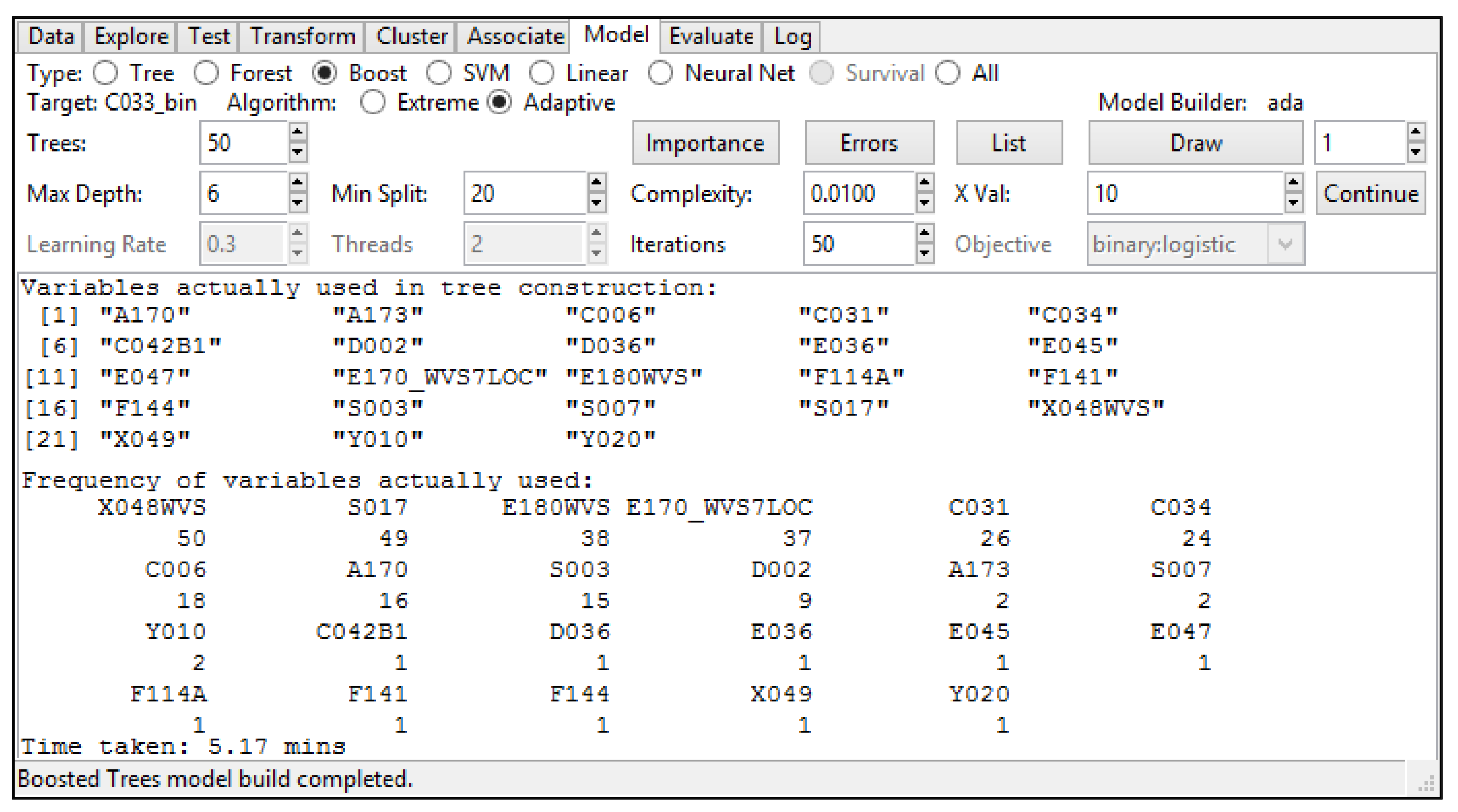
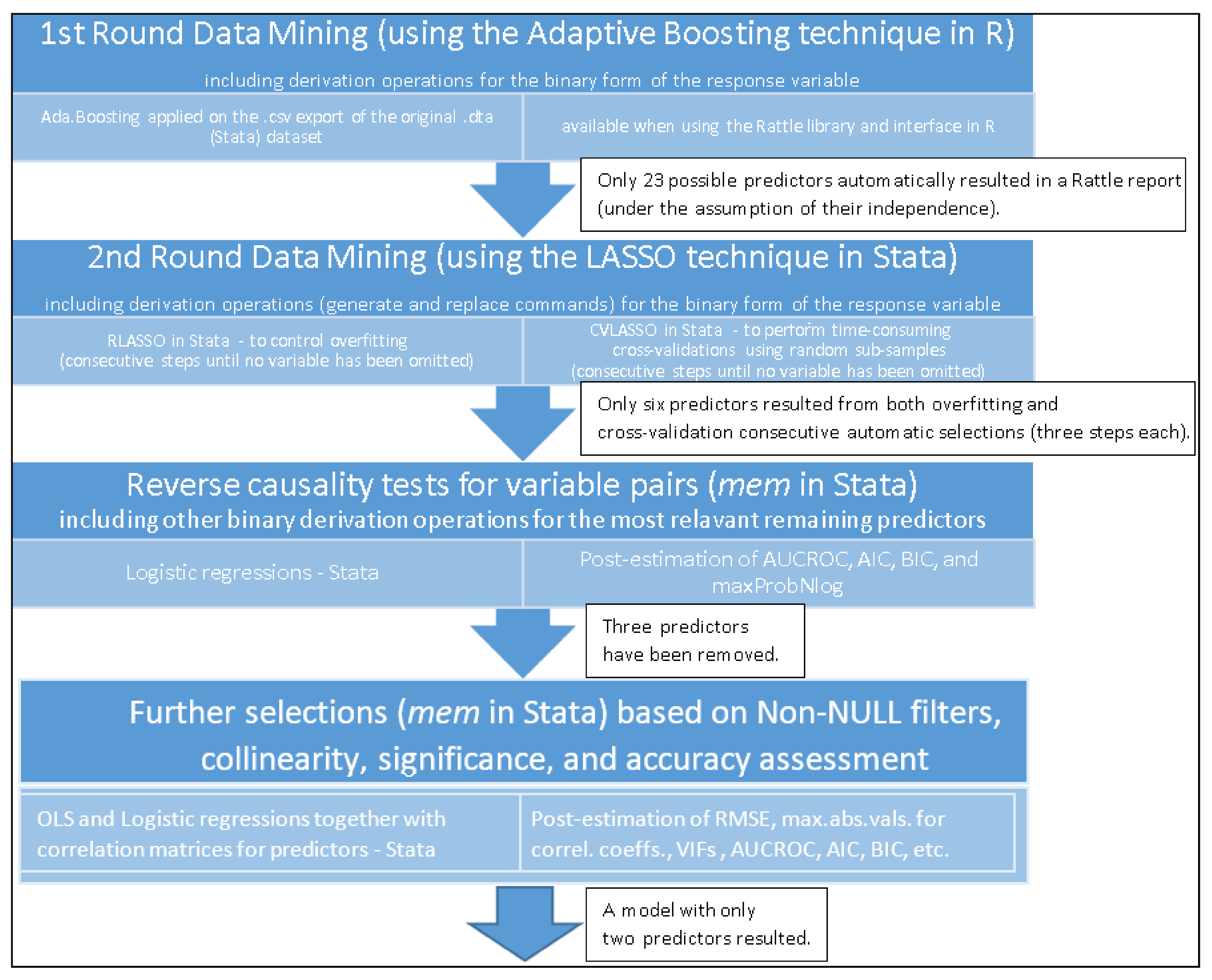
6. Conclusions
Author Contributions
Funding
Institutional Review Board Statement
Data Availability Statement
Acknowledgments
Conflicts of Interest
Appendix A
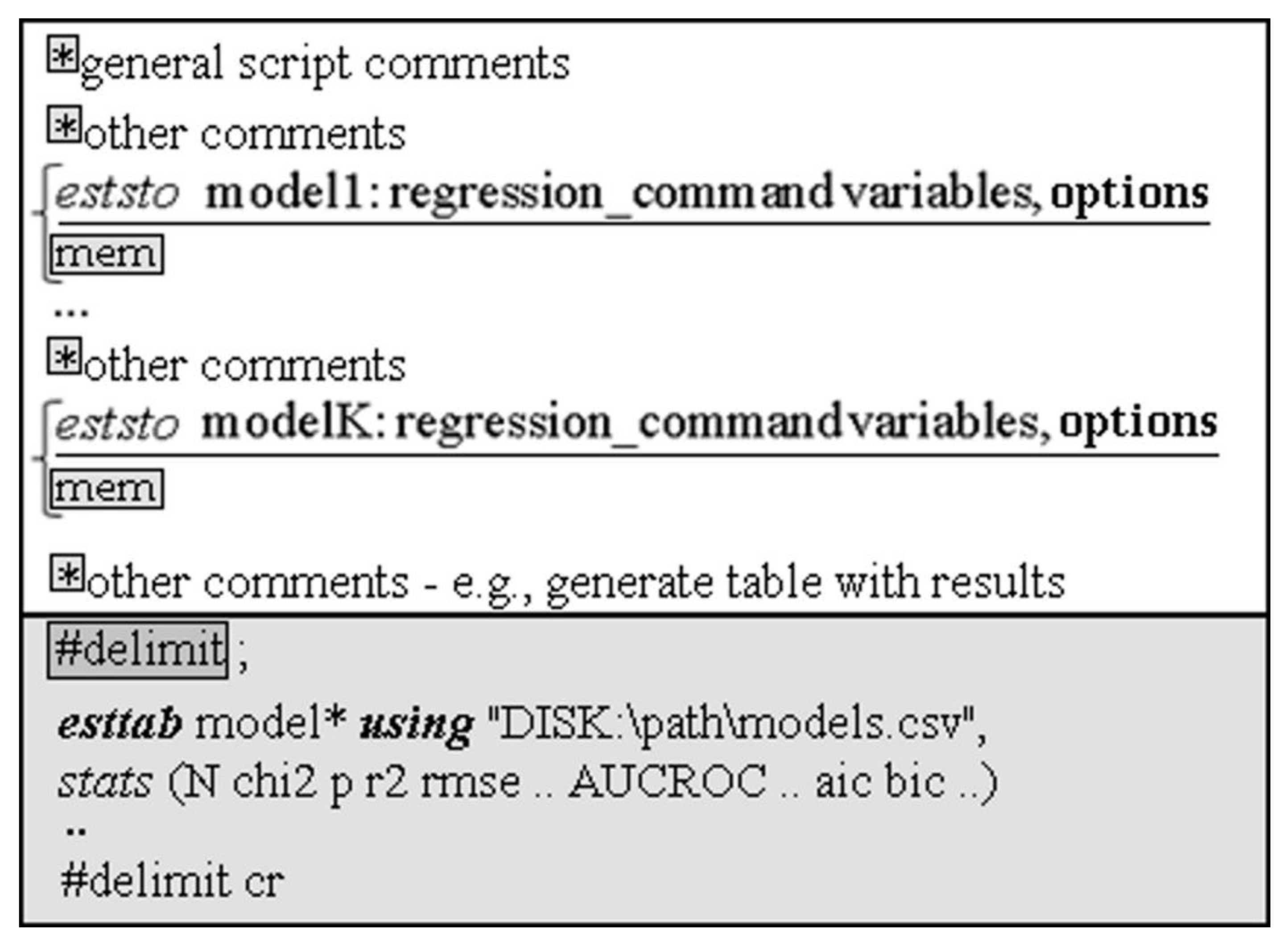
| 1 *Processing script needed to argue the utility of the mem tool in Stata 2 use “F:\WVS_TimeSeries_stata_v1_6.dta” 3 label list C033 4 generate C033_bin = . 5 replace C033_bin = 1 if C033! = . & C033> = 6 6 replace C033_bin = 0 if C033! = . & C033<6 & C033>0 7 ***On the variables selected by Adaptive Boosting (R, the Rattle library) we apply LASSO as follows:*** 8 rlasso C033_bin A170 A173 C006 C031 C034 C042B1 D002 D036 E036 E045 E047 E170_WVS7LOC E180WVS F114A F141 F144 S003 S007 S017 X048WVS X049 Y010 Y020 9 cvlasso C033_bin A170 A173 C006 C031 C034 C042B1 D002 D036 E036 E045 E047 E170_WVS7LOC E180WVS F114A F141 F144 S003 S007 S017 X048WVS X049 Y010 Y020 10 cvlasso, lse 11 ***both rlasso & cvlasso with the lse option (1st LASSO stage above) remove 12 everything except: A170 A173 C006 C031 C034 C042B1 D002 12 rlasso C033_bin A170 A173 C006 C031 C034 C042B1 D002 13 cvlasso C033_bin A170 A173 C006 C031 C034 C042B1 D002 14 cvlasso, lse 15 ***cvlasso, lse (2nd LASSO stage above) removes A173 after running the previous three command lines*** 16 rlasso C033_bin A170 C006 C031 C034 C042B1 D002 17 cvlasso C033_bin A170 C006 C031 C034 C042B1 D002 18 cvlasso, lse 19 ***cv lasso, lse and rlasso (3rd LASSO stage above) do not eliminate anything (no loss)*** 20 label list A170 21 generate A170_bin = . 22 replace A170_bin = 1 if A170! = . & A170> = 6 23 replace A170_bin = 0 if A170! = . & A170<6 & A170>0 24 label list C006 25 generate C006_bin = . 26 replace C006_bin = 1 if C006! = . & C006> = 6 27 replace C006_bin = 0 if C006! = . & C006<6 & C006>0 28 label list C031 29 generate C031_bin = . 30 replace C031_bin = 1 if C031! = . & C031< = 2 & C031>0 31 replace C031_bin = 0 if C031! = . & C031>2 32 label list C034 33 generate C034_bin = . 34 replace C034_bin = 1 if C034! = . & C034> = 6 35 replace C034_bin = 0 if C034! = . & C034<6 & C034>0 36 *C042B1 is already in a binary form 37 label list C042B1 38 *Therefore, we did not perform any derivation in this case above. 39 label list D002 40 generate D002_bin = . 41 replace D002_bin = 1 if D002! = . & D002> = 6 42 replace D002_bin = 0 if D002! = . & D002<6 & D002>0 43 *Save the resulting dataset (after the processing above) 44 save “F:\WVS_TimeSeries_stata_v1_6processed.dta”, replace 45 *Open the resulting dataset above 46 clear all 47 cls 48 use “F:\WVS_TimeSeries_stata_v1_6processed.dta” |
| 1 *! version 1.1 24August2022 2 *Authors: Daniel HOMOCIANU & Cristina TIRNAUCA 3 *Download “mem.ado” to C:\ado\personal (Run it after any regression by simply using mem) 4 program define mem//(Model Evaluation Metrics) 5 version 17.0 6 ***Section1:Extracting the predictors’s list plus other specs.(e.g., condition) upto 1st comma’s position(cpos) from a regression command 7 capture local cpos = strpos(ustrright(e(cmdline),strlen(e(cmdline))-(strpos(e(cmdline),e(depvar))+strlen(e(depvar)))),”,”) 8 if _rc = = 0 { 9 if ‘cpos’ = = 0 { 10 local prdlist_plus = ustrright(e(cmdline),strlen(e(cmdline))-(strpos(e(cmdline),e(depvar))+strlen(e(depvar)))) 11 } 12 if ‘cpos’>0 { 13 local prdlist_plus = ustrleft(ustrright(e(cmdline),strlen(e(cmdline))-(strpos(e(cmdline),e(depvar))+strlen(e(depvar)))),‘cpos’-1) 14 } 15 } 16 ***Section2:Computing and storing maxAbsVPMCC = max.Abs.Value from Predictors’Matrix with Correl.Coefficient 17 ***https://doi.org/10.1213/ane.0000000000002864 18 capture correlate ‘prdlist_plus’ 19 if _rc = = 0 { 20 matrix crlv = vec(r(C)) 21 local lim = rowsof(crlv) 22 local maxAbsVPMCC = 0 23 foreach i of num 1/‘lim’ { 24 if abs(crlv[‘i’,1])! = 1 { 25 local maxAbsVPMCC = max(‘maxAbsVPMCC’,abs(crlv[‘i’,1])) 26 } 27 } 28 if ‘maxAbsVPMCC’ = = 0 { 29 local maxAbsVPMCC = . 30 } 31 estadd local maxAbsVPMCC “‘:di %6.4f ‘maxAbsVPMCC’’” 32 } 33 ***Section3:Computing and storing the Variance Inflation Factors (VIFs)—both OLS model’s max.accepted & max.computed VIFs 34 ***https://dx.doi.org/10.4172%2F2161-1165.1000227 35 ***and also AUC(ROC), chi^2 and p for Goodness of Fit (GOF) 36 if e(cmd) = = “regress” { 37 local OLSmaxAcceptVIF = 1/(1-e(r2)) 38 estadd local OLSmaxAcceptVIF “‘:di %6.4f ‘OLSmaxAcceptVIF’’” 39 capture estat vif 40 if _rc = = 0 { 41 local OLSmaxComputVIF = ‘r(vif_1)’ 42 estadd local OLSmaxComputVIF “‘:di %6.4f ‘OLSmaxComputVIF’’” 43 } 44 } 45 capture lroc, nograph 46 if _rc = = 0 { 47 local AUCROC = ‘r(area)’ 48 estadd local AUCROC “‘:di %6.4f ‘AUCROC’’” 49 } 50 capture estat gof 51 if _rc = = 0 { 52 capture local chi2GOF = ‘r(chi2)’ 53 if _rc = = 0 { 54 estadd local chi2GOF “‘:di %6.2f ‘chi2GOF’’” 55 } 56 capture local pGOF = ‘r(p)’ 57 if _rc = = 0 { 58 estadd local pGOF “‘:di %6.4f ‘pGOF’’” 59 } 60 } 61 ***Section4:Storing last 2 thresholds for maxProbNlog(max.probability on the X axis from Zlotnik&Abraira’s nomogram gen.-nomolog) 62 ***https://doi.org/10.1177%2F1536867 × 1501500212 63 if e(cmd) = = “logit” | e(cmd) = = “logistic” { 64 set graphics off 65 capture nomolog 66 capture local maxProbNlogPenultThrsh = P [1,colsof(P)-1] 67 if _rc = = 0 { 68 estadd local maxProbNlogPenultThrsh “‘:di %6.4f ‘maxProbNlogPenultThrsh’’” 69 } 70 capture local maxProbNlogLastThrsh = P [1,colsof(P)] 71 if _rc = = 0 { 72 estadd local maxProbNlogLastThrsh “‘:di %6.4f ‘maxProbNlogLastThrsh’’” 73 } 74 set graphics on 75 } 76 end |
| 1 *! version 1.1 24August20222 2 *Authors: Daniel HOMOCIANU & Cristina TIRNAUCA 3 *Ex.1: mem4pp, dopath(“C:/Table3_rev_cause_checks_logit.do”) *Ex.2: mem4pp, dopath(“C:/Table5_comp_perf_checks.do”) xcpu(6) disk(“C”) 4 program define mem4pp 5 version 17.0 6 syntax, dopath(string) [xcpu(real 2) disk(string)] 7 ***Getting the path of the current dataset and its number of variables*** 8 local dataset = “‘c(filename)’” 9 local dsetnvars = ‘c(k)’+150 10 if ‘dsetnvars’ < 2048 { 11 local dsetnvars = 2048 12 } 13 if ‘dsetnvars’ > 120000 { 14 di as error “ Error: The dataset is too large (>120000 vars.)!” 15 exit 16 } 17 if missing(“‘dataset’”) { 18 di as error “ Error: First you must open a dataset!” 19 exit 20 } 21 ***Checking the existing CPU configuration on the local hardware*** 22 local nproc : env NUMBER_OF_PROCESSORS 23 local xc = 2 24 if !missing(“‘xcpu’”) { 25 if ‘xcpu’> = 2 & ‘xcpu’< = ‘nproc’ { 26 local xc = int(‘xcpu’) 27 } 28 else { 29 di as error “ Error: Provide at least 2 logical CPU cores (but no more than ‘nproc’) for MP tasks!” 30 exit 31 } 32 } 33 local dsk = “C” 34 if !missing(“‘disk’”) { 35 if “‘disk’”< = “z” | “‘disk’”< = “Z” { 36 local dsk = “‘disk’” 37 } 38 else { 39 di as error “Error: Provide a valid disk letter!” 40 exit 41 } 42 } 43 di “MEM4PP will save the results in the .csv files at ‘dsk’:\StataPPtasks!” 44 ***Generating the “main_do_pp_file.do” parallel processing template file*** 45 local smpt_path = “‘dsk’:\StataPPtasks\” 46 shell rd “‘smpt_path’”/s/q 47 qui mkdir “‘smpt_path’” 48 local full_do_path = “‘smpt_path’\main_do_pp_file.do” 49 local q_subdir = “queue” 50 qui mkdir ‘”‘smpt_path’/‘q_subdir’”‘ 51 local queue_path = “‘smpt_path’\‘q_subdir’” 52 local l_subdir = “logs” 53 qui mkdir ‘”‘smpt_path’/‘l_subdir’”‘ 54 local logs_path = “‘smpt_path’\‘l_subdir’” 55 qui file open mydofile using ‘”‘full_do_path’”‘, write replace 56 file write mydofile “clear all” _n 57 file write mydofile “log using “ 58 file write mydofile ‘”““‘ 59 file write mydofile “‘logs_path’\log” 60 file write mydofile “‘” 61 file write mydofile “1” 62 file write mydofile “‘“ 63 file write mydofile “.txt” 64 file write mydofile ‘”““‘ 65 file write mydofile “, text” _n 66 file write mydofile “set maxvar ‘dsetnvars’” _n 67 file write mydofile “use “ 68 file write mydofile ‘”““‘ 69 file write mydofile “‘dataset’” 70 file write mydofile ‘”““‘ _n 71 file write mydofile “‘” 72 file write mydofile “2” 73 file write mydofile “‘“ 74 file write mydofile “, “ 75 file write mydofile “‘” 76 file write mydofile “3” 77 file write mydofile “‘“ _n 78 file write mydofile “mem” _n 79 file write mydofile “esttab model* using “ 80 file write mydofile ‘”““‘ 81 file write mydofile “‘smpt_path’\model” 82 file write mydofile “‘” 83 file write mydofile “1” 84 file write mydofile “‘“ 85 file write mydofile “.csv” 86 file write mydofile ‘”““‘ 87 file write mydofile “, stats(N chi2 p r2 r2_p rmse maxAbsVPMCC OLSmaxAcceptVIF OLSmaxComputVIF AUCROC pGOF chi2GOF aic bic maxProbNlogPenultThrsh maxProbNlogLastThrsh) cells(b (star fmt(4)) se(par fmt(4))) starlevels(* 0.05 ** 0.01 *** 0.001)” _n 88 file write mydofile “log close” 89 qui file close mydofile 90 ***Finding the Stata directory*** 91 local _sys = “‘c(sysdir_stata)’” 92 local exec : dir “‘_sys’” files “Stata*.exe” , respect 93 foreach exe in ‘exec’ { 94 if inlist(“‘exe’”,”Stata.exe”,”Stata-64.exe”,”StataMP.exe”,”StataMP-64.exe”,”StataSE.exe”,”StataSE-64.exe”) { 95 local curr_st_exe ‘exe’ 96 continue, break 97 } 98 } 99 local st_path = “‘_sys’”+”‘curr_st_exe’” 100 capture confirm file ‘”‘_sys’‘curr_st_exe’”‘ 101 if _rc ! = 0 { 102 di as error “Stata’s sys dir and executable NOT found!” 103 exit 104 } 105 else { 106 di “!!!Stata’s sys dir and executable found: ‘st_path’ !!!” 107 } 108 ***Dynamically generating and configuring .do files(tasks) using “main_do_pp_file.do”*** 109 local k = 0 110 file open myfile using “‘dopath’”, read 111 file read myfile line 112 while r(eof) = = 0 { 113 if “‘ = word(“‘line’”,1)’” = = “#delimit” { 114 continue, break 115 } 116 if “‘ = word(“‘line’”,1)’”! = “mem” & substr(“‘ = word(“‘line’”,1)’”,1,1)! = “*” { 117 local k = ‘k’ + 1 118 capture local cpos = strpos(“‘line’”,”,”) 119 if ‘cpos’ = = 0 { 120 local l_line = “‘line’” 121 local r_line = ““ 122 } 123 if ‘cpos’>0 { 124 local l_line = ustrleft(“‘line’”, ‘cpos’-1) 125 local r_line = ustrright(“‘line’”, length(“‘line’”)-‘cpos’-1) 126 } 127 if ‘k’<10 { 128 qui file open mydofile using ‘queue_path’\job0‘k’.do, write replace 129 qui file write mydofile ‘”do “‘dsk’:\StataPPtasks\main_do_pp_file.do” “0‘k’” “‘l_line’” “‘r_line’”“‘ 130 } 131 if ‘k’> = 10 { 132 qui file open mydofile using ‘queue_path’\job‘k’.do, write replace 133 qui file write mydofile ‘”do “‘dsk’:\StataPPtasks\main_do_pp_file.do” “‘k’” “‘l_line’” “‘r_line’”“‘ 134 } 135 file close mydofile 136 } 137 file read myfile line 138 } 139 file close myfile 140 ***Allocating .do tasks to logical CPU cores using qsub v.13.1 (06/10/2015), made by Adrian Sayers.*** 141 *ssc install qsub, replace 142 if ‘xc’>‘k’ { 143 local xc = ‘k’ 144 } 145 qsub , jobdir(‘queue_path’) maxproc(‘xc’) statadir(‘st_path’) deletelogs 146 ***Printing logs for all .do tasks in the main session’s console*** 147 local mylogs : dir “‘logs_path’” files “*.txt” 148 local k = 0 149 foreach entry in ‘mylogs’ { 150 local k = ‘k’ + 1 151 if ‘k’<10 { 152 type “‘logs_path’\log0‘k’.txt” 153 } 154 if ‘k’> = 10 { 155 type “‘logs_path’\log‘k’.txt” 156 } 157 } 158 end |


| Variable | Question | Coding |
|---|---|---|
| C033 | Job satisfaction—DEPENDENT VARIABLE | 1-Dissatisfied … 10-Satisfied |
| C033_bin | Job satisfaction (binary format)—DEPENDENT VARIABLE | 1 if C033! = . & C033> = 6 |
| 0 if C033! = . & C033<6 & C033>0 | ||
| A170 | Satisfaction with your life | 1-Dissatisfied … 10-Satisfied |
| A170_bin | Satisfaction with your life (binary format) | 1 if A170! = . & A170> = 6 |
| 0 if A170! = . & A170<6 & A170>0 | ||
| C006 | Satisfaction with the financial situation of household | 1-Dissatisfied … 10-Satisfied |
| C006_bin | Satisfaction with the financial situation of household (binary format) | 1 if C006! = . & C006> = 6 |
| 0 if C006! = . & C006<6 & C006>0 | ||
| C031 | Degree of pride in your work | 1-A great deal … 4-None |
| C031_bin | Degree of pride in your work (binary format) | 1 if C031! = . & C031< = 2 & C031>0 |
| 0 if C031! = . & C031>2 | ||
| C034 | Freedom of decision-taking in the job | 1-Not at all … 10-A great deal |
| C034_bin | Freedom of decision-taking in the job (binary format) | 1 if C034! = . & C034> = 6 |
| 0 if C034! = . & C034<6 & C034>0 | ||
| C042B1 | Why people work: work is like a business transaction | 0-Not mentioned, 1-Mentioned |
| D002 | Satisfaction with home life | 1-Dissatisfied … 10-Satisfied |
| D002_bin | Satisfaction with home life (binary format) | 1 if D002! = . & D002> = 6 |
| 0 if D002! = . & D002<6 & D002>0 |
| Variable | N | Mean | Std.Dev. | Min | 0.25 | Median | 0.75 | Max |
|---|---|---|---|---|---|---|---|---|
| C033 | 15,968 | 7.27 | 2.31 | 1 | 6 | 8 | 9 | 10 |
| C033_bin | 15,968 | 0.77 | 0.42 | 0 | 1 | 1 | 1 | 1 |
| A170 | 420,669 | 6.7 | 2.42 | 1 | 5 | 7 | 8 | 10 |
| A170_bin | 420,669 | 0.69 | 0.46 | 0 | 0 | 1 | 1 | 1 |
| C006 | 411,461 | 5.75 | 2.58 | 1 | 4 | 6 | 8 | 10 |
| C006_bin | 411,461 | 0.54 | 0.5 | 0 | 0 | 1 | 1 | 1 |
| C031 | 14,988 | 1.73 | 0.87 | 1 | 1 | 2 | 2 | 4 |
| C031_bin | 14,988 | 0.51 | 0.5 | 0 | 0 | 1 | 1 | 1 |
| C034 | 17,900 | 6.54 | 2.79 | 1 | 5 | 7 | 9 | 10 |
| C034_bin | 17,900 | 0.65 | 0.48 | 0 | 0 | 1 | 1 | 1 |
| C042B1 | 22,493 | 0.14 | 0.35 | 0 | 0 | 0 | 0 | 1 |
| D002 | 25,653 | 7.72 | 2.24 | 1 | 7 | 8 | 10 | 10 |
| D002_bin | 25,653 | 0.83 | 0.38 | 0 | 1 | 1 | 1 | 1 |
| Model | (1) | (2) | (3) | (4) | (5) | (6) | (7) | (8) | (9) | (10) | (11) | (12) |
|---|---|---|---|---|---|---|---|---|---|---|---|---|
| Predictors/Response Var. | C033_bin | A170_bin | C033_bin | C006_bin | C033_bin | C031_bin | C033_bin | C034_bin | C033_bin | C042B1 | C033_bin | D002_bin |
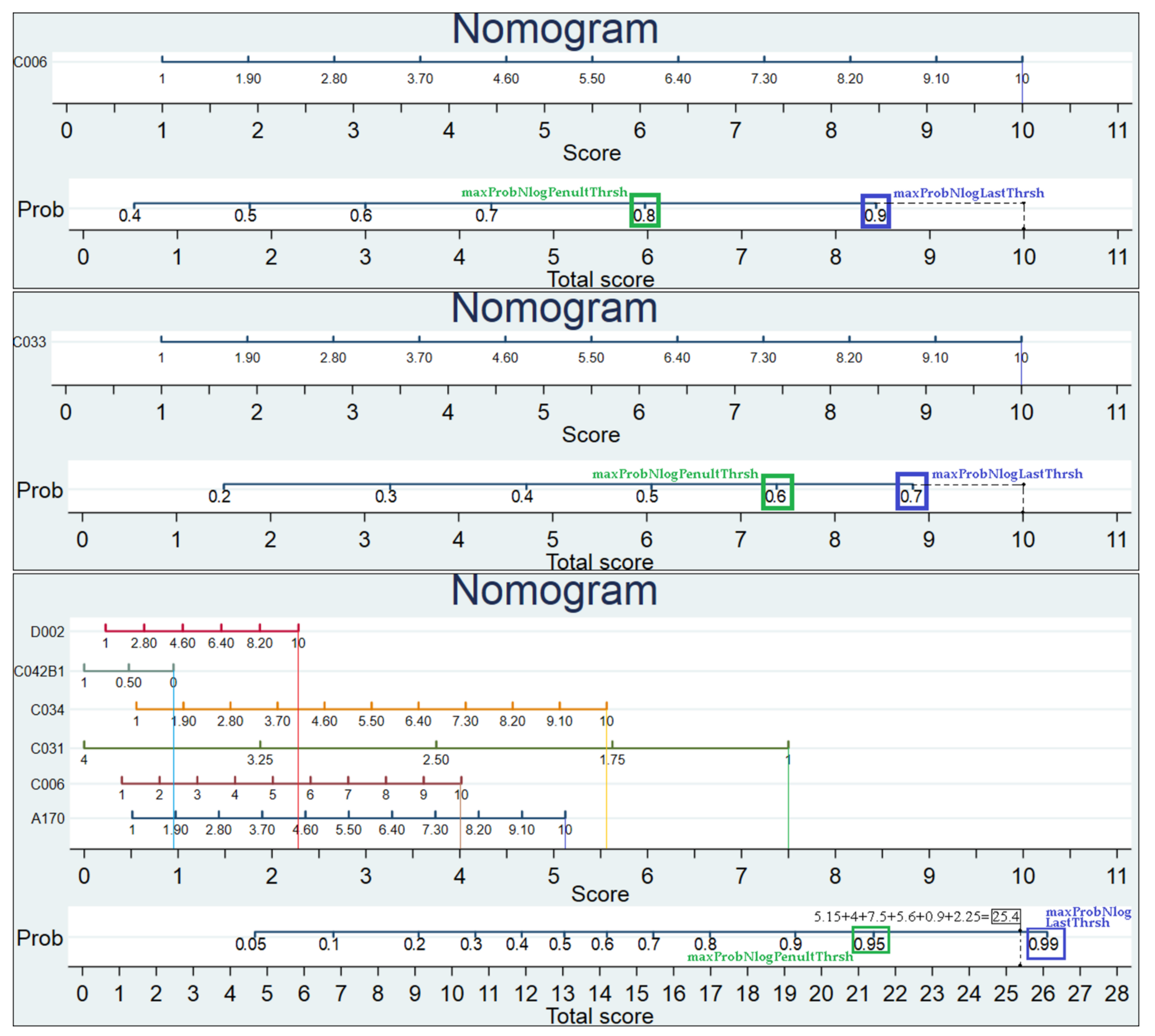
| A170 | 0.3973 *** | |||||||||||
| −0.0097 | ||||||||||||
| C006 | 0.3300 *** | |||||||||||
| −0.0084 | ||||||||||||
| C031 | −1.2461 *** | |||||||||||
| −0.0263 | ||||||||||||
| C034 | 0.3233 *** | |||||||||||
| −0.0077 | ||||||||||||
| C042B1 | −0.7301 *** | |||||||||||
| −0.0508 | ||||||||||||
| D002 | 0.3264 *** | |||||||||||
| −0.0092 | ||||||||||||
| C033 | 0.3480 *** | 0.3049 *** | 0.5306 *** | 0.3800 *** | −0.1425 *** | 0.3360 *** | ||||||
| −0.0089 | −0.0081 | −0.0118 | −0.0088 | −0.0099 | −0.0096 | |||||||
| _cons | −1.3840 *** | −1.2868 *** | −0.5840 *** | −1.8448 *** | 3.5825 *** | −1.8024 *** | −0.7322 *** | −1.9542 *** | 1.3594 *** | −0.6646 *** | −1.1913 *** | −0.6141 *** |
| −0.0646 | −0.0618 | −0.0473 | −0.0604 | −0.0576 | −0.0729 | −0.0475 | −0.0638 | −0.0233 | −0.0705 | −0.069 | −0.0644 | |
| N | 15,848 | 15,848 | 15,811 | 15,811 | 14,900 | 14,900 | 15,811 | 15,811 | 13,528 | 13,528 | 15,752 | 15,752 |
| chi^2 | 1681.697 | 1511.46 | 1558.748 | 1406.843 | 2237.2495 | 2034.758 | 1771.526 | 1851.932 | 206.4193 | 208.5788 | 1253.118 | 1212.24 |
| p | 0 | 0 | 0 | 0 | 0 | 0 | 0 | 0 | 0 | 0 | 0 | 0 |
| pseudo R^2 | 0.1258 | 0.106 | 0.1046 | 0.08 | 0.1833 | 0.2168 | 0.1244 | 0.1204 | 0.0135 | 0.0178 | 0.088 | 0.0993 |
| AUC-ROC | 0.7443 | 0.7129 | 0.7272 | 0.6797 | 0.7667 | 0.8095 | 0.7377 | 0.728 | 0.5548 | 0.5927 | 0.6912 | 0.7193 |
| AIC | 14,832.35 | 15,908.21 | 15,176.62 | 19,733.43 | 13,249.447 | 10,656.06 | 14,786.66 | 17,607.53 | 14,307.509 | 11,673.32 | 15,391.21 | 12,641.82 |
| BIC | 14,847.69 | 15,923.55 | 15,191.96 | 19,748.77 | 13,264.665 | 10,671.28 | 14,802 | 17,622.87 | 14,322.534 | 11,688.34 | 15,406.54 | 12,657.15 |
| maxProbNlogPenultThrsh | 0.8 | 0.7 | 0.8 | 0.6 | 0.9 | 0.9 | 0.8 | 0.7 | ··· . | 0.2 | 0.7 | 0.8 |
| maxProbNlogLastThrsh | 0.9 | 0.8 | 0.9 | 0.7 | 0.95 | 0.95 | 0.9 | 0.8 | 0.7 | 0.3 | 0.8 | 0.9 |
| Model | (1) | (2) | (3) |
|---|---|---|---|
| Predictors/Response Var. | C033_bin | ||
| A170 | 0.0512 *** | 0.0536 *** | |
| −0.0017 | −0.0015 | ||
| C006 | 0.0338 *** | 0.0409 *** | |
| −0.0014 | −0.0013 | ||
| C034 | 0.0433 *** | 0.0451 *** | |
| −0.0013 | −0.0013 | ||
| _cons | 0.2089 *** | 0.1061 *** | 0.2267 *** |
| −0.0123 | −0.0125 | −0.0111 | |
| N | 15704 | 15705 | 15671 |
| p | 0 | 0 | 0 |
| R^2 | 0.1697 | 0.2111 | 0.1906 |
| RMSE | 0.3814 | 0.371 | 0.3759 |
| maxAbsVPMCC | 0.5643 | 0.2765 | 0.2759 |
| OLSmaxAcceptVIF | 1.2043 | 1.2676 | 1.2355 |
| OLSmaxComputVIF | 1.2797 | 1.0873 | 1.0882 |
| AIC | 14,298.3711 | 13,423.0338 | 13,806.915 |
| BIC | 14,321.3561 | 13,446.019 | 13,829.8937 |
| Model | (1) | (2) | (3) | (4) | (5) | (6) | (7) | (8) | (9) | (10) | (11) | (12) |
|---|---|---|---|---|---|---|---|---|---|---|---|---|
| Regression Type | logit | OLS | logit | OLS | logit | logit | OLS | OLS | logit | logit | OLS | OLS |
| Filter Condition | N/A | N/A | N/A | N/A | if C006! = . | if A170! = . | if C006! = . | if A170! = . | N/A | N/A | N/A | N/A |
| Predictors/Response Var. | C033_bin | |||||||||||
| A170 | 0.1802 *** | 0.0244 *** | 0.2667 *** | 0.0416 *** | 0.3433 *** | 0.0535 *** | 0.3441 *** | 0.0536 *** | ||||
| −0.0141 | −0.0019 | −0.0111 | −0.0017 | −0.0103 | −0.0016 | −0.0102 | −0.0015 | |||||
| C006 | 0.1413 *** | 0.0166 *** | 0.1851 *** | 0.0254 *** | 0.2780 *** | 0.0409 *** | 0.2776 *** | 0.0409 *** | ||||
| −0.0122 | −0.0015 | −0.0102 | −0.0014 | −0.0092 | −0.0013 | −0.0091 | −0.0013 | |||||
| C031 | −0.8791 *** | −0.1425 *** | ||||||||||
| −0.0305 | −0.0047 | |||||||||||
| C034 | 0.1957 *** | 0.0261 *** | 0.2579 *** | 0.0394 *** | 0.2784 *** | 0.2765 *** | 0.0432 *** | 0.0449 *** | 0.2791 *** | 0.2768 *** | 0.0433 *** | 0.0451 *** |
| −0.0099 | −0.0014 | −0.0084 | −0.0013 | −0.0083 | −0.0081 | −0.0013 | −0.0013 | −0.0083 | −0.0081 | −0.0013 | −0.0013 | |
| C042B1 | −0.3345 *** | −0.0523 *** | ||||||||||
| −0.0653 | −0.0092 | |||||||||||
| D002 | 0.0803 *** | 0.0123 *** | ||||||||||
| −0.0136 | −0.002 | |||||||||||
| _cons | −0.7354 *** | 0.4882 *** | −3.1023 *** | 0.0649 *** | −2.7134 *** | −1.9714 *** | 0.1076 *** | 0.2276 *** | −2.7222 *** | −1.9723 *** | 0.1061 *** | 0.2267 *** |
| −0.1383 | −0.0219 | −0.0866 | −0.0127 | −0.0813 | −0.0672 | −0.0126 | −0.0112 | −0.081 | −0.0669 | −0.0125 | −0.0111 | |
| N | 12,899 | 12,899 | 15,576 | 15,576 | 15,576 | 15,576 | 15,576 | 15,576 | 15,705 | 15,671 | 15,705 | 15,671 |
| chi2 | 2477.4685 | 2541.0448 | 2376.3159 | 2285.7133 | 2400.0313 | 2306.7919 | ||||||
| p | 0 | 0 | 0 | 0 | 0 | 0 | 0 | 0 | 0 | 0 | 0 | 0 |
| R^2 | 0.2997 | 0.2279 | 0.2101 | 0.19 | 0.2111 | 0.1906 | ||||||
| pseudo R^2 | 0.2927 | 0.2231 | 0.2021 | 0.1842 | 0.203 | 0.1846 | ||||||
| RMSE | 0.3487 | 0.3668 | 0.371 | 0.3757 | 0.371 | 0.3759 | ||||||
| maxAbsVPMCC | 0.5264 | 0.5264 | 0.4696 | 0.4696 | 0.2763 | 0.2754 | 0.2763 | 0.2754 | 0.2765 | 0.2759 | 0.2765 | 0.2759 |
| OLSmaxAcceptVIF | 1.4279 | 1.2951 | 1.2659 | 1.2346 | 1.2676 | 1.2355 | ||||||
| OLSmaxComputVIF | 1.5845 | 1.3203 | 1.0872 | 1.0878 | 1.0873 | 1.0882 | ||||||
| AUC−ROC | 0.852 | 0.8166 | 0.8022 | 0.7919 | 0.8028 | 0.7922 | ||||||
| p GOF | 0.0017 | 0 | 0 | 0 | 0 | 0 | ||||||
| chi^2 GOF | 7159.82 | 1155.72 | 283.98 | 256.74 | 280.01 | 260.9 | ||||||
| AIC | 9709.2467 | 9434.8801 | 12,902.2457 | 12,963.9656 | 13,249.4442 | 13,546.3796 | 13,317.1563 | 13,707.6119 | 13,353.616 | 13,640.0974 | 13,423.0338 | 13,806.915 |
| BIC | 9761.501 | 9487.1345 | 12,932.8596 | 12,994.5796 | 13,272.4047 | 13,569.3401 | 13,340.1168 | 13,730.5724 | 13,376.6012 | 13,663.0761 | 13,446.019 | 13,829.8937 |
| maxProbNlogPenultThrsh | 0.95 | 0.9 | 0.9 | 0.9 | 0.9 | 0.9 | ||||||
| maxProbNlogLastThrsh | 0.99 | 0.95 | 0.95 | 0.95 | 0.95 | 0.95 | ||||||
References
- Haghish, E.F. Markdoc: Literate Programming in Stata. Stata J. 2016, 16, 964–988. [Google Scholar] [CrossRef]
- Jiménez-Valverde, A. Insights into the area under the receiver operating characteristic curve (AUC) as a discrimination measure in species distribution modelling. Glob. Ecol. Biogeogr. 2012, 21, 498–507. [Google Scholar] [CrossRef]
- Rolke, W.; Gongora, C.G. A chi-square goodness-of-fit test for continuous distributions against a known alternative. Comput. Stat. 2021, 36, 1885–1900. [Google Scholar] [CrossRef]
- Vatcheva, K.P.; Lee, M.J.; McCormick, J.B.; Rahbar, M.H. Multi-collinearity in Regression Analyses Conducted in Epidemiologic Studies. Epidemiology 2016, 6, 227. [Google Scholar]
- Gao, Y.; Cowling, M. Introduction to Panel Data, Multiple Regression Method, and Principal Components Analysis Using Stata: Study on the Determinants of Executive Compensation—A Behavioral Approach Using Evidence from Chinese Listed Firms; SAGE Publications Ltd.: Thousand Oaks, CA, USA, 2019. [Google Scholar]
- De Luca, G.; Magnus, J.R. Bayesian model averaging and weighted-average least squares: Equivariance, stability, and numerical issues. Stata J. Promot. Commun. Stat. Stata 2011, 11, 518–544. [Google Scholar] [CrossRef]
- Rajiah, K.; Sivarasa, S.; Maharajan, M.K. Impact of Pharmacists’ Interventions and Patients’ Decision on Health Outcomes in Terms of Medication Adherence and Quality Use of Medicines among Patients Attending Community Pharmacies: A Systematic Review. Int. J. Environ. Res. Public Health 2021, 18, 4392. [Google Scholar] [CrossRef]
- Homocianu, D.; Plopeanu, A.-P.; Ianole-Calin, R. A Robust Approach for Identifying the Major Components of the Bribery Tolerance Index. Mathematics 2021, 9, 1570. [Google Scholar] [CrossRef]
- Sadeghi, A.R.; Bahadori, Y. Urban Sustainability and Climate Issues: The Effect of Physical Parameters of Streetscape on the Thermal Comfort in Urban Public Spaces; Case Study: Karimkhan-e-Zand Street, Shiraz, Iran. Sustainability 2021, 13, 10886. [Google Scholar] [CrossRef]
- Thanh, M.T.G.; Van Toan, N.; Toan, D.T.T.; Thang, N.P.; Dong, N.Q.; Dung, N.T.; Hang, P.T.T.; Anh, L.Q.; Tra, N.T.; Ngoc, V.T.N. Diagnostic Value of Fluorescence Methods, Visual Inspection and Photographic Visual Examination in Initial Caries Lesion: A Systematic Review and Meta-Analysis. Dent. J. 2021, 9, 30. [Google Scholar] [CrossRef] [PubMed]
- Wang, L.; Ling, C.-H.; Lai, P.-C.; Huang, Y.-T. Can The ‘Speed Bump Sign’ Be a Diagnostic Tool for Acute Appendicitis? Evidence-Based Appraisal by Meta-Analysis and GRADE. Life 2022, 12, 138. [Google Scholar] [CrossRef] [PubMed]
- Von Hippel, P.T. How many imputations do you need? A two-stage calculation using a quadratic rule. Sociol. Methods Res. 2018, 49, 699–718. [Google Scholar] [CrossRef]
- Fávero, L.P.; Belfiore, P.; Santos, M.A.; Souza, R.F. Overdisp: A Stata (and Mata) package for direct detection of overdispersion in Poisson and negative binomial regression models. Stat. Optim. Inf. Comput. 2020, 8, 773–789. [Google Scholar] [CrossRef]
- Nyaga, V.N.; Arbyn, M. Metadta: A Stata command for meta-analysis and meta-regression of diagnostic test accuracy data—A tutorial. Arch. Public Health 2022, 80, 95. [Google Scholar] [CrossRef]
- Weber, S.; Péclat, M.; Warren, A. Travel distance and travel time using Stata: New features and major improvements in georoute. Stata J. Promot. Commun. Stat. Stata 2022, 22, 89–102. [Google Scholar] [CrossRef]
- Peterson, L.E. MLOGITROC: Stata Module to Calculate Multiclass ROC Curves and AUC from Multinomial Logistic Regression; Statistical Software Components S457181; Boston College Department of Economics: Chestnut Hill, MA, USA, 2010. [Google Scholar]
- Bilger, M. Overfit: Stata Module to Calculate Shrinkage Statistics to Measure Overfitting as Well as out- and in-Sample Predictive Bias; Statistical Software Components S457950; Boston College Department of Economics: Chestnut Hill, MA, USA, 2015. [Google Scholar]
- Zlotnik, A.; Abraira, V. A general-purpose nomogram generator for predictive logistic regression models. Stata J. 2015, 15, 537–546. [Google Scholar] [CrossRef]
- Watson, I. Tabout: Stata Module to Export Publication Quality Cross-Tabulations; Statistical Software Components S447101; Boston College Department of Economics: Chestnut Hill, MA, USA, 2004. [Google Scholar]
- Jann, B. Making regression tables from stored estimates. Stata J. 2005, 5, 288–308. [Google Scholar] [CrossRef]
- Jann, B. Making regression tables simplified. Stata J. 2007, 7, 227–244. [Google Scholar] [CrossRef]
- Oancea, B.; Dragoescu, R.M. Integrating R and Hadoop for Big Data Analysis, Romanian Statistical Review. arXiv 2014, arXiv:1407.4908. [Google Scholar]
- Meng, X.; Bradley, J.; Yavuz, B.; Sparks, E.; Venkataraman, S.; Liu, D.; Freeman, J.; Tsai, D.B.; Amde, M.; Owen, S.; et al. MLlib: Machine Learning in Apache Spark. arXiv 2015, arXiv:1505.06807. [Google Scholar]
- Fotache, M.; Cluci, M.-I. Big Data Performance in private clouds. In Some initial findings on Apache Spark Clusters deployed in OpenStack. In Proceedings of the 2021 20th RoEduNet Conference: Networking in Education and Research (RoEduNet), Iasi, Romania, 4–6 November 2021. [Google Scholar]
- Murty, C.S.; Saradhi Varma, G.P.; Satyanarayana, C. Content-based collaborative filtering with hierarchical agglomerative clustering using user/item based ratings. J. Interconnect. Netw. 2022, 22, 2141026. [Google Scholar] [CrossRef]
- Alhussan, A.A.; AlEisa, H.N.; Atteia, G.; Solouma, N.H.; Seoud, R.A.; Ayoub, O.S.; Ghoneim, V.F.; Samee, N.A. ForkJoinPcc algorithm for computing the PCC matrix in gene co-expression networks. Electronics 2022, 11, 1174. [Google Scholar] [CrossRef]
- Vega Yon, G.G.; Quistorff, B. PARALLEL: A command for parallel computing. Stata J. 2019, 19, 667–684. [Google Scholar] [CrossRef]
- Ditzen, J. MULTISHELL: Stata Module to Allot Do Files and Variations of Loops Across Parallel Instances of Windows Stata and Computers Efficiently; Statistical Software Components S458512; Boston College Department of Economics: Chestnut Hill, MA, USA, 2018. [Google Scholar]
- Sayers, A. QSUB: Stata Module to Emulate a Cluster Environment Using Your Desktop PC. EconPapers. 2017. Available online: https://EconPapers.repec.org/RePEc:boc:bocode:s458366 (accessed on 1 July 2022).
- Karabulut, E.M.; Ibrikci, T. Analysis of Cardiotocogram Data for Fetal Distress Determination by Decision Tree-Based Adaptive Boosting Approach. J. Comput. Commun. 2014, 2, 32–37. [Google Scholar] [CrossRef]
- Schonlau, M. Boosted regression (boosting): An introductory tutorial and a Stata plugin. Stata J. 2005, 5, 330–354. [Google Scholar] [CrossRef]
- Tibshirani, R. Regression shrinkage and selection via the LASSO. J. R. Stat. Soc. Ser. B 1996, 58, 267–288. [Google Scholar] [CrossRef]
- Sanchez, J.D.; Rêgo, L.C.; Ospina, R. Prediction by Empirical Similarity via Categorical Regressors. Mach. Learn. Knowl. Extr. 2019, 1, 38. [Google Scholar] [CrossRef]
- Ahrens, A.; Hansen, C.B.; Schaffer, M.E. Lassopack: Model selection and prediction with regularized regression in Stata. Stata J. Promot. Commun. Stat. Stata 2020, 20, 176–235. [Google Scholar] [CrossRef]
- Acuña, E.; Rodriguez, C. The Treatment of missing values and its effect on classifier accuracy. In Classification, Clustering, and Data Mining Applications. Studies in Classification, Data Analysis, and Knowledge Organisation; Banks, D., McMorris, F.R., Arabie, P., Gaul, W., Eds.; Springer: Berlin, Germany, 2004; pp. 639–647. [Google Scholar]
- Jann, B.; Long, J.S. Tabulating SPost results using estout and esttab. Stata J. 2010, 10, 46–60. [Google Scholar] [CrossRef]
- Plopeanu, A.-P.; Homocianu, D.; Florea, N.; Ghiuță, O.-A.; Airinei, D. Comparative Patterns of Migration Intentions: Evidence from Eastern European Students in Economics from Romania and Republic of Moldova. Sustainability 2019, 11, 4935. [Google Scholar] [CrossRef]
- Homocianu, D.; Plopeanu, A.-P.; Florea, N.; Andrieș, A.M. Exploring the Patterns of Job Satisfaction for Individuals Aged 50 and over from Three Historical Regions of Romania. An Inductive Approach with Respect to Triangulation, Cross-Validation and Support for Replication of Results. Appl. Sci. 2020, 10, 2573. [Google Scholar] [CrossRef]
- King, G.; Roberts, M.E. How Robust Standard Errors Expose Methodological Problems They Do Not Fix, and What to Do about It. Polit. Anal. 2015, 23, 159–179. [Google Scholar] [CrossRef]
- Mukaka, M.M. A guide to appropriate use of Correlation coefficient in medical research. Malawi Med. J. 2012, 24, 69–71. [Google Scholar] [PubMed]
- Schober, P.; Boer, C.; Schwarte, L.A. Correlation coefficients: Appropriate use and interpretation. Anesth. Analg. 2018, 126, 1763–1768. [Google Scholar] [CrossRef] [PubMed]
- Freund, R.J.; Wilson, W.J.; Sa, P. Regression Analysis: Statistical Modeling of a Response Variable, 2nd ed.; Academic Press: Cambridge, MA, USA, 2006. [Google Scholar]
- Tokuda, Y.; Fujii, S.; Inoguchi, T. Individual and Country-Level Effects of Social Trust on Happiness: The Asia Barometer Survey. In Trust with Asian Characteristics. Trust (Interdisciplinary Perspectives); Inoguchi, T., Tokuda, Y., Eds.; Springer: Singapore, 2017; Volume 1. [Google Scholar] [CrossRef]
- Munafò, M.R.; Smith, G.D. Robust research needs many lines of evidence. Nature 2018, 553, 399–401. [Google Scholar] [CrossRef] [PubMed]
- Airinei, D.; Homocianu, D. The Importance of Video Tutorials for Higher Education—The Example of Business Information Systems. In Proceedings of the 6th International Seminar on the Quality Management in Higher Education, Tulcea, Romani, 8–9 July 2010; Available online: https://ssrn.com/abstract=2381817 (accessed on 1 July 2022).
- Homocianu, D.; Airinei, D. PCDM and PCDM4MP: New Pairwise Correlation-Based Data Mining Tools for Parallel Processing of Large Tabular Datasets. Mathematics 2022, 10, 2671. [Google Scholar] [CrossRef]
- Luo, J.; Gao, F.; Liu, J.; Wang, G.; Chen, L.; Fagan, A.M.; Day, G.S.; Vöglein, J.; Chhatwal, J.P.; Xiong, C.; et al. Statistical estimation and comparison of group-specific bivariate correlation coefficients in family-type clustered studies. J. Appl. Stat. 2021, 49, 2246–2270. [Google Scholar] [CrossRef] [PubMed]
- Dang, X.; Nguyen, D.; Chen, Y.; Zhang, J. A new Gini correlation between quantitative and qualitative variables. Scand. J. Stat. 2020, 48, 1314–1343. [Google Scholar] [CrossRef]


Publisher’s Note: MDPI stays neutral with regard to jurisdictional claims in published maps and institutional affiliations. |
© 2022 by the authors. Licensee MDPI, Basel, Switzerland. This article is an open access article distributed under the terms and conditions of the Creative Commons Attribution (CC BY) license (https://creativecommons.org/licenses/by/4.0/).
Share and Cite
Homocianu, D.; Tîrnăucă, C. MEM and MEM4PP: New Tools Supporting the Parallel Generation of Critical Metrics in the Evaluation of Statistical Models. Axioms 2022, 11, 549. https://doi.org/10.3390/axioms11100549
Homocianu D, Tîrnăucă C. MEM and MEM4PP: New Tools Supporting the Parallel Generation of Critical Metrics in the Evaluation of Statistical Models. Axioms. 2022; 11(10):549. https://doi.org/10.3390/axioms11100549
Chicago/Turabian StyleHomocianu, Daniel, and Cristina Tîrnăucă. 2022. "MEM and MEM4PP: New Tools Supporting the Parallel Generation of Critical Metrics in the Evaluation of Statistical Models" Axioms 11, no. 10: 549. https://doi.org/10.3390/axioms11100549
APA StyleHomocianu, D., & Tîrnăucă, C. (2022). MEM and MEM4PP: New Tools Supporting the Parallel Generation of Critical Metrics in the Evaluation of Statistical Models. Axioms, 11(10), 549. https://doi.org/10.3390/axioms11100549