Article

Change Point Detection Using Penalized Multidegree Splines

Department of Information Statistics, Chungbuk National University, Cheongju 28644, Chungbuk, Korea
*
Author to whom correspondence should be addressed.
These authors contributed equally to this work.
Axioms 2021, 10(4), 331; https://doi.org/10.3390/axioms10040331
Submission received: 13 October 2021 / Revised: 24 November 2021 / Accepted: 29 November 2021 / Published: 1 December 2021

Abstract

:
We consider a function estimation method with change point detection using truncated power spline basis and elastic-net-type L 1 -norm penalty. The L 1 -norm penalty controls the jump detection and smoothness depending on the value of the parameter. In terms of the proposed estimators, we introduce two computational algorithms for the Lagrangian dual problem (coordinate descent algorithm) and constrained convex optimization problem (an algorithm based on quadratic programming). Subsequently, we investigate the relationship between the two algorithms and compare them. Using both simulation and real data analysis, numerical studies are conducted to validate the performance of the proposed method.

1. Introduction

A nonparametric function estimation is useful for estimating the actual relationship of data exhibiting nonlinear relationships. It is a statistical method for estimating the relationship between variables based on observed data, assuming that the actual function representing the relationships between input variables and response variables belongs to an infinite-dimensional parametric space. Representative examples, including kernel density estimation (chapter 1 of [1]), local polynomials [2], splines (pp. 118–180 of [3]) and curve estimation (chapter 2 of [4]), have been investigated previously.
A representative method used for function estimation is the basis function method. Among the basis function methods, splines are the most frequently used. In function estimation, an infinite number of parameters cannot be estimated using a finite amount of data. Therefore, function estimation is performed by introducing a function space and a basis function. If the function space and basis function are defined, then the shape of the function to be estimated using the basis function as a predictor variable can be expressed as a linear combination of the basis functions spanning the appropriate function space. Therefore, the function estimation problem can be regarded as estimating the regression coefficients.
Among the many basis functions used to interpolate data or fit smooth curves, the spline basis is the most typically used. The spline basis function is defined as a piecewise polynomial that is differentiable for every knot spacing. Its main underlying technology is truncated power splines (see chapter 3 of [5]). Additionally, it offers the advantages of simple construction and easy interpretation of the model parameters. However, in model with many overlapping intervals, basis functions are highly correlated. Therefore, several computational problems may occur when the number of knots increases significantly because the predictor matrix for the truncated power spline basis becomes dense. Consequently, incorrect fitting may occur (chapter 7 of [6]).
In the basis function methodology, the objective function to be optimized is a convex function. The coordinate descent algorithm (CDA) [7] is simple, efficient and useful for optimizing these objective functions. The concept of the algorithm is to optimize the solution of a problem involving the minimization (maximization) of a convex (concave) function for a multidimensional vector. Coefficient updates keep the remaining coefficients constant. The objective function is regarded as a one-dimensional function. Tseng [8] proved that the coordinate descent converges when a convex penalty term is non-differentiable but separable in each coordinate. This result implies that the coordinate-wise algorithms for the least absolute shrinkage and selection operator (lasso) [9], group lasso [10] and elastic net [11] converge to their optimal solutions. Another simpler method to obtain the optimal solution is to use quadratic programming (QP) [12]. QP is a type of nonlinear programming that obtains a mathematical optimization problem involving quadratic functions.
The selection of knots and the detection of change points in regression splines significantly affect the performance of the model. Knot selection and change point detection methods have been studied extensively. Osbone et al. [13] proposed an algorithm that allows an efficient computation of the lasso estimator for knot selection to be performed. Leitenstorfer and Tutz [14] considered the boosting technique to select variables in knot selection. Garton [15] proposed a method for selecting the number and position of knots using Gaussian and non-Gaussian data. Aminikhanhahi and Cook [16] proposed a change point detection method for time-series data. Meanwhile, Tibshirani et al. [17] proposed sparsity and smoothness using a fused lasso.
The main contributions of this study are as follows.
First, a new type of function estimator is established for change points in the nonparametric regression function estimation model. The proposed function estimator is defined by a linear combination of multidegree-based splines to simultaneously provide a change point detection and smoothing.
Second, two computational algorithms are introduced to address the constrained convex optimization problem (algorithm based on QP) and Lagrangian dual problem (CDA); moreover, the relationship between them is investigated. Numerical studies using both simulated and real datasets are provided to demonstrate the performance of the proposed method.
Herein, we present a new statistical learning methodology for modeling and analyzing data to address the change point detection problem. The proposed method involves two tuning parameters that control the penalty terms. We express the estimator as a linear combination of a polynomial and a truncated power-spline basis for zero and positive integer degrees, respectively. The coefficients are estimated using a CDA to minimize the residual sum of squares and QP. We consider three sets of simulation data to measure the performance of the proposed method and conduct an analysis on real data with changes or jump point(s).
This paper is organized as follows: In Section 2, we present a nonparametric regression model containing observed data and the penalized regression spline estimator. The process of updating the coefficients based on the CDA and the estimated coefficients obtained using QP is presented in Section 3. Additionally, the estimators obtained using the two methods are compared and their characteristics are introduced briefly. In Section 4, using the simulation and real data, we validate the performance of our proposed model. In Section 5, we summarize the conclusions of this study. All codes implemented using the software program R for numerical analysis are available as Supplementary Materials.

2. Model and Estimator

Consider a nonparametric regression model
y i = f ( x i ) + ε i for i = 1 , , n ,
where { x i } ’s I R are the predictors and { y i } ’s R are responses. The model is nonparametric because it does not contain any parametric assumptions regarding f. Model (1) is expressed similarly as the conditional expectation E ( Y | X = x ) . In this case, ε 1 , , ε n are only required to satisfy the property that the expected value is zero with positive variance σ 2 and no distribution assumption is required. Without loss of generality, we write I = [ 0 , 1 ] hereinafter for notational simplicity.
Because it is impossible to estimate an infinite number of parameters using a finite amount of data, a specific function space for estimation should be considered. In nonparametric estimation, it is typically assumed that f belongs to a massive class of functions [1]. In this study, because the goal is to achieve a smooth function estimation that can detect change point(s), the function space to which f belongs can be specified as follows.
Let F K be the space of spline functions of mixed degrees 0 and positive integer d > 0 with K interior knots 0 = t 0 < t 1 < < t K < t K + 1 = 1 . Therefore, any function f F K can be expressed as
f ( x ; θ ) = α 0 + j = 1 d α j x j + k = 1 K β k P 0 , k ( x ) + γ k P d , k ( x ) ,
where θ = ( α , β , γ ) with α = ( α 0 , α 1 , , α d ) , β = ( β 1 , , β K ) , γ = ( γ 1 , , γ K ) ,
P 0 , k ( x ) = 1 if x > t k 0 otherwise and P d , k ( x ) = ( x t k ) + d for k = 1 , , K .
It is noteworthy that ( a ) + is a function that assumes a real value of a if a > 0 and 0 otherwise. We first select the number of the initial knots K for the splines and then place them at the same interval within ( 0 , 1 ) . Generally, one may select a sufficiently large value of Kn, or n / 2 , for example—to select data-adaptive knots.
The empirical risk of θ is defined as
R ( θ ) = 1 2 n i = 1 n y i f ( x i ; θ ) 2 .
The penalized objective function to be minimized is expressed as
R λ , τ ( θ ) = R ( θ ) + λ τ β 1 + ( 1 τ ) γ 1
for λ > 0 , τ [ 0 , 1 ] and · 1 , the L 1 -norm. The penalty term is the concept of elastic-net penalty [11]. Similar to the lasso, λ reduces only β and γ . Furthermore, similar to an elastic net, τ is a tuning parameter that controls the relative penalty. If τ is of a higher value, then a greater weight is assigned to the L 1 -norm of β , where the jump detection penalty is. By contrast, if τ is of a lower value, then a greater weight is assigned to the L 1 -norm of γ , which is a penalty indicating the function smoothness.
Let
θ ^ λ , τ = argmin θ R λ , τ ( θ )
and define the multidegree spline estimator (MDSE) as
f ^ = f · ; θ ^ .

3. Implementation

Specifically in mathematical statistics fields, penalized regression problems can seek to optimize a multivariate quadratic function subject to linear constraints on the regression coefficients. To realize the proposed estimator, two computational methods are considered, i.e., the CDA and the algorithm for QP, using the quadprog package [18] in the R program. We describe the abovementioned two methods comprehensively and present their advantages and disadvantages. Both methods are implemented using the software program R.

3.1. CDA

The CDA optimizes the objective function with respect to a single coefficient at a time, iteratively cycling through all coefficients until convergence is reached. We adopt the CDA introduced by Jhong et al. (2017) to perform univariate smoothing for each coefficient. Because the objective function (2) is convex for θ , one can adopt the CDA to obtain the MDSE. This algorithm is inspired by the studies of Friedman et al. [19] and Jhong et al. [20]. However, it is a new attempt, in that the proposed algorithm is applied to the elastic net penalty considering two hyper parameters, λ and τ .
For j = 0 , 1 , 2 , , d and k = 1 , 2 , , K , let α ˜ j , β ˜ k and γ ˜ k denote the initial (or updated) values. Specifically,
α ˜ = α ˜ 0 , α ˜ 1 , , α ˜ d R 1 + d , β ˜ = β ˜ 1 , , β ˜ K R K ,
and γ ˜ = γ ˜ 1 , , γ ˜ K R K . For notational convenience, we use
θ ˜ = ( α ˜ , β ˜ , γ ˜ ) = ( θ ˜ 1 , , θ ˜ J ) for J = 1 + d + 2 K .
Therefore, the coordinate descent update is written in the following forms:
θ ˜ j argmin θ j R R λ , τ θ ˜ 1 , , θ ˜ j 1 , θ j , θ ˜ j + 1 , , θ ˜ J for j = 1 , , J .

3.1.1. Updating α

The optimization problem for α j , j = 0 , 1 , , d has a quadratic form. Hence, we can solve this problem by transforming the objective function for α j into a perfect square form. It is noteworthy that x i 0 = 1 .
R λ , τ α ˜ 0 , , α ˜ j 1 , α j , α ˜ j + 1 , , α ˜ d , β ˜ , γ ˜ = 1 2 n i = 1 n y i j α ˜ x i α j x i j k = 1 K β ˜ k P 0 , k x i + γ ˜ k P d , k x i 2 + λ τ k = 1 K | β ˜ k | + λ 1 τ k = 1 K | γ ˜ k | = 1 2 n i = 1 n r i , α ( j ) α j x i j 2 + ( terms   independent   for   α j ) = i = 1 n x i j 2 2 n α j i = 1 n r i , α ( j ) x i j i = 1 n x i j 2 2 + ( terms   independent   for   α j ) ,
where
r i , α ( j ) = y i j α ˜ x i k = 1 K β ˜ k P 0 , k x i k = 1 K γ ˜ k P d , k x i
is a partial residual. Because α j is not subject to penalization, one can update each coefficient systematically using the partial residual. Therefore, we update
α ˜ j i = 1 n r i , α ( j ) x i j i = 1 n x i j 2 for j = 0 , 1 , , d .

3.1.2. Updating β and γ

Unlike updating α , one cannot use only the partial residual to update β and γ , because the objective function contains the penalty terms. Hence, we used the soft-thresholding operator [19] to solve the lasso solutions. The soft-thresholding operator is defined as
S y , λ = y λ if y > λ y + λ if y < λ 0 otherwise for y R and λ > 0 .
We select k { 1 , , K } and transform the objective function for β k into a quadratic form. Subsequently,
R λ , τ α ˜ , β ˜ 1 , , β ˜ k 1 , β k , β ˜ k + 1 , , β ˜ K , γ ˜ = 1 2 n i = 1 n y i j = 0 d α ˜ j x i j k β ˜ P 0 , x i β k P 0 , k x i = 1 K γ ˜ P d , x i 2 + λ τ k | β ˜ | + λ τ | β k | + λ 1 τ = 1 K | γ ˜ | = 1 2 n i = 1 n r i , β ( k ) β k P 0 , k x i 2 + λ τ | β k | + ( terms   independent   for   β k ) ,
where
r i , β ( k ) = y i j = 0 d α ˜ j x i j k β ˜ P 0 , x i = 1 K γ ˜ P d , x i .
Finally, using the soft-thresholding operator, we can update β ˜ k as follows:
β ˜ k S 1 n i = 1 n r i , β ( k ) P 0 , k x i , λ τ 1 n i = 1 n P 0 , k x i 2 .
Similarly, γ ˜ k is expressed as
γ ˜ k S 1 n i = 1 n r i , γ ( k ) P d , k x i , λ 1 τ 1 n i = 1 n P d , k x i 2 for k = 1 , , K .

3.1.3. Algorithm Details

Algorithm 1 shows the process of computing the proposed estimator using the CDA. We implement the code using the software program R. For the observed data, we create a basis matrix B to fit to our model.
B = 1 X 1 X d P 0 P d R n × 1 + d + 2 K ,
where 1 = 1 1 R n , X j = x 1 j x n j R n for j = 1 , d .
P 0 = P 0 , 1 P 0 , K R n × K , and P d = P d , 1 P d , K R n × K . After B is created, we select the tuning parameters. We compute λ m a x , which is the smallest value that causes all coefficients to be zero, as follows:
λ m a x = max k 1 n | P 0 , k x , y | , 1 n | P d , k x , y | ,
where x , y = i = 1 n x i y i for n-dimensional vectors x and y, respectively. Thereafter, we generate candidates for the two tuning parameters λ and τ , respectively.
For the case involving λ , the equally spaced candidates decrease from log ( λ m a x ) to log ( λ m a x × λ m i n _ m a x _ r a t i o ) for a maximum of n λ times, which is the number of λ candidates. λ m i n _ m a x _ r a t i o is the ratio of the maximum and minimum values of λ , which is a sufficiently low positive value. Subsequently, it is reconverted to the exponential scale and the last candidate value is replaced with a zero. Next, in the case of τ , we generate n τ values from 0 to 1 at equal intervals.
Subsequently, we compute the value of the initial objective function as i = 1 n y i 2 / 2 n . Thereafter, we begin updating all the coefficients until that is achieved. Finally, we select the best model among n λ × n τ models. In statistical data analysis, some representative information criteria exist, such as the Akaike information criterion (AIC; [21]), the Bayesian information criterion (BIC) and cross validation (CV). In general, the AIC and CV involve the selection of a model with a relatively large variance and small bias compared with the BIC. Because the purpose of this study is to accurately select significant change points, we use the BIC [22], which involves the selection of a model with a relatively small variance, defined as follows:
B I C = n log 2 × R λ , τ ( θ ^ ) + p log n ,
where p is the number of non-zero coefficients. We select the best model that minimized the BIC. For a detailed calculation of the degrees of freedom p in penalized regression model, see [9].
Algorithm 1: Coordinate descent algorithm (CDA).
Axioms 10 00331 i001

3.2. Quadratic Programming

The disadvantage of the CDA is that the computational cost increases with the higher number of iterations. Therefore, we use a new algorithm, i.e., QP, to compute the proposed estimator. In QP, certain mathematical optimization problems involving quadratic functions are solved. In this regard, a multivariate quadratic function subject to linear constraints on the coefficients can be minimized. Hence, because the solution can be obtained without iterations, QP demonstrates computational advantage over the CDA.
The Lagrangian dual problem (2) is converted into the constraint optimization problem, such that
θ ^ = α ^ , β ^ , γ ^ = argmin θ R θ subject   to τ | | β | | 1 + 1 τ | | γ | | 1 t ,
where t 0 . For u R , let
u + = u if u 0 0 if u < 0 and u = u if u 0 0 if u > 0 .
Therefore, u = u + u and | u | = u + + u . By reparameterizating β k and γ k ,
β k = β k + β k , | β k | = β k + + β k ,
γ k = γ k + γ k , | γ k | = γ k + + γ k
Therefore, the optimization problem is equivalent to minimizing
1 2 n i = 1 n y i j = 0 d α j x i j k = 1 K ( β k ) + ( β k ) P 0 , k ( x i ) + ( γ k ) + ( γ k ) P d , k ( x i ) 2
subject to
τ k = 1 K ( β k ) + + ( β k ) + 1 τ k = 1 K ( γ k ) + + ( γ k ) t ,
in addition to 4 × K non-negativity constraints
( β k ) + 0 , ( β k ) 0 , ( γ k ) + 0 , ( γ k ) 0 f o r k = 1 , , K .
Next, we define
Z = 1 X 1 X d P 0 P 0 P d P d R n × ( 1 + d + 4 K )
and
b = α β + β γ + γ R 1 + d + 4 K ,
where β + = { ( β k ) + } , β = { ( β k ) } , γ + = { ( γ k ) + } , and γ = { ( γ k ) } . Subsequently,
R ( θ ) = 1 2 n ( y Z b ) ( y Z b ) = 1 2 n y y 1 n y Z b + 1 2 n b ( Z Z ) b .
Hence, the minimization problem is equivalent to
min b 1 n y Z b + 1 2 n b ( Z Z ) b
subject to
0 ( 1 + d ) × 1 0 ( 1 + d ) × K 0 ( 1 + d ) × K 0 ( 1 + d ) × K 0 ( 1 + d ) × K τ K × 1 I K × K 0 K × K 0 K × K 0 K × K τ K × 1 0 K × K I K × K 0 K × K 0 K × K ( 1 τ ) K × 1 0 K × K 0 K × K I K × K 0 K × K ( 1 τ ) K × 1 0 K × K 0 K × K 0 K × K I K × K α β + β γ + γ t 0 K × 1 0 K × 1 0 K × 1 0 K × 1 ,
where τ K × 1 = ( τ , , τ ) R K and ( 1 τ ) K × 1 = ( ( 1 τ ) , , ( 1 τ ) ) R K . Hence, the problem can be computed via QP.
In R, the solve.QP function in the quadprog package [18] provides the solution for QP problems that involve minimizing ( dvec x + 1 / 2 x Dmat x ) with respect to x with constraints Amat x bvec . Dmat is the matrix that appears in the quadratic function to be minimized. dvec is the vector that appears in the quadratic function to be minimized. bvec is the vector that has the values of the constraints. Amat is the matrix that defines the constraints for minimizing the quadratic function. Therefore, in our case, the matrices and vectors defined above correspond to
Dmat 1 n ( Z Z ) , dvec 1 n y Z , bvec t 0 4 K × 1
and
Amat 0 ( 1 + d ) × 1 0 ( 1 + d ) × K 0 ( 1 + d ) × K 0 ( 1 + d ) × K 0 ( 1 + d ) × K τ K × 1 I K × K 0 K × K 0 K × K 0 K × K τ K × 1 0 K × K I K × K 0 K × K 0 K × K ( 1 τ ) K × 1 0 K × K 0 K × K I K × K 0 K × K ( 1 τ ) K × 1 0 K × K 0 K × K 0 K × K I K × K .
It is noteworthy that a small positive vector is added to the diagonal entries of 1 n ( Z Z ) to guarantee a positive definite matrix and prevent numerical computational issues.
Finally, the solution of b obtained via QP is defined as
b ^ = α ^ β ^ + β ^ γ ^ + γ ^ ,
and the MDSE is expressed as
β ^ k = ( β ^ k ) + ( β ^ k ) , and γ ^ k = ( γ ^ k ) + ( γ ^ k ) for k = 1 , , K .

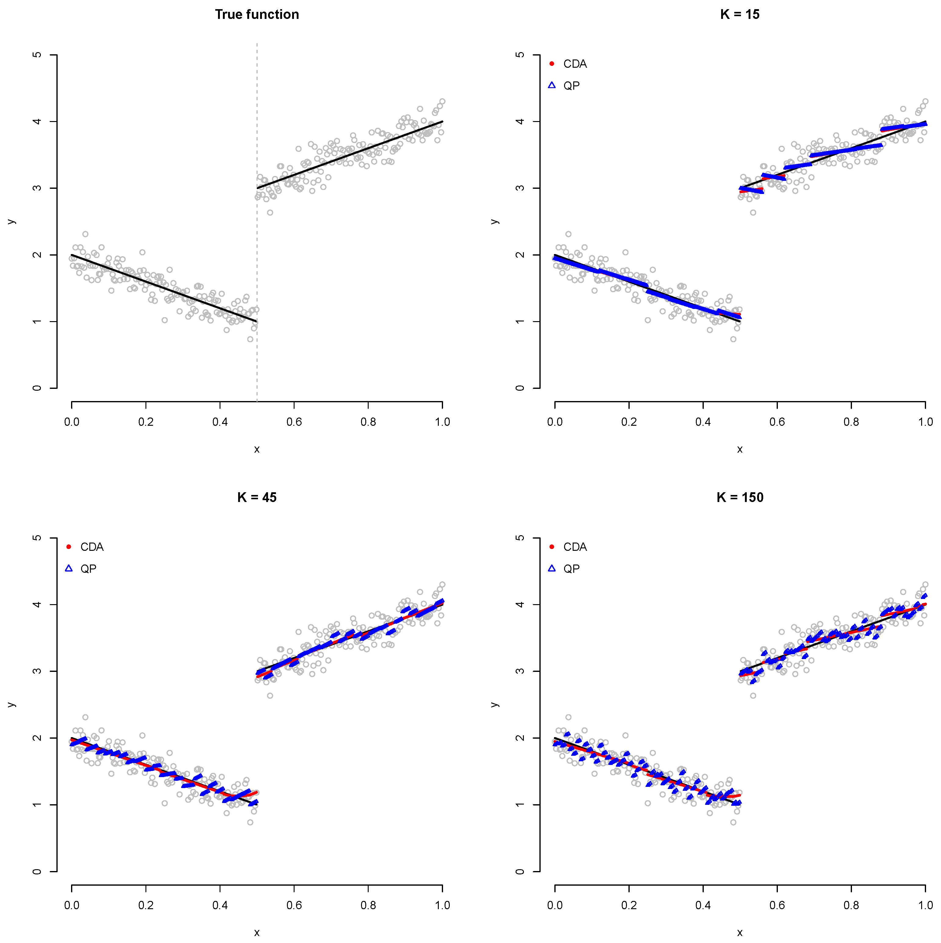
3.3. Comparison between CDA and QP

We introduce two computational algorithms to solve the constrained convex optimization problem (algorithm based on QP) and the Lagrangian dual problem (CDA); subsequently, we investigate the relationship between them.
First, we verify that the CDA estimator and the estimator obtained via QP are identical. Subsequently, a simulation is performed using the sample size n = 300 with one true knot of 0.5, as shown in Figure 1.
In this simulation, the settings used for the CDA yield zero for all the initial coefficients, with n λ = 50 (the number of λ ), n τ = 10 (the number of τ ), d = 1 (the non-zero degree), ϵ = 1 × 10 10 (stopping criterion) and R = 5000 (maximum iteration). Using λ and τ obtained from the best CDA model, the corresponding tuning parameter t required for QP is obtained as follows:
t = λ τ k = 1 K | β ^ k | + λ 1 τ k = 1 K | γ ^ k | .
The above relation can be derived using the Karush–Kuhn–Tucker (KKT) optimality condition [23] based on the sub-gradient [24], since the L 1 -norm penalty term cannot be differentiated with respect to the coefficients.
The remaining options are set to the same value and then are simulated. As shown in Figure 1, we confirm that both algorithms yield the same results. However, when the number of knots (K) increases, the CDA does not converge appropriately to the minimum under a limited iteration number (M) and the stopping criterion ( ϵ ), unlike QP. Hence, we performe the next simulation using only QP. It is noteworthy that a higher number K of interior knots indicates a higher probability of overfitting.

4. Numerical Analysis
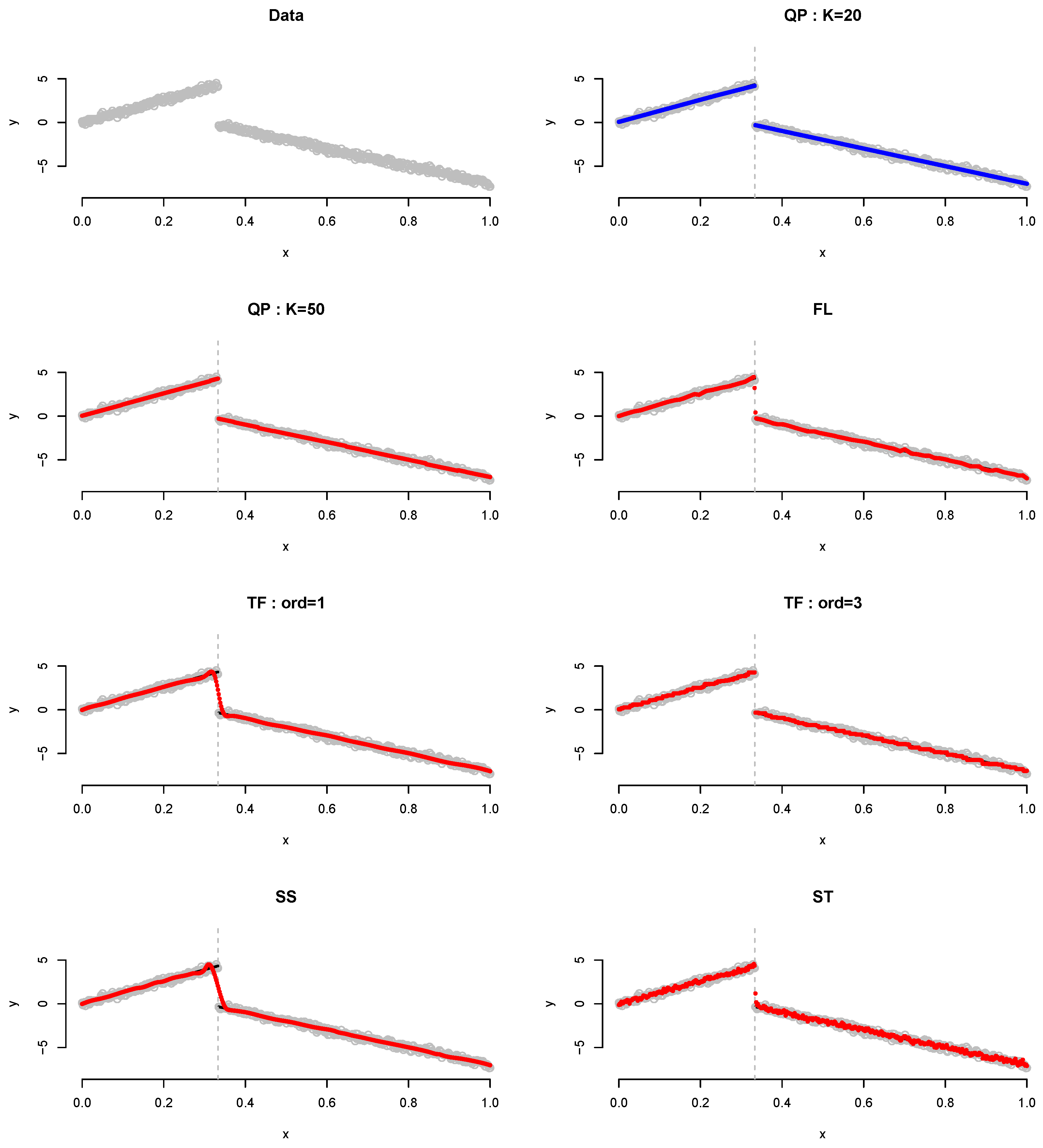
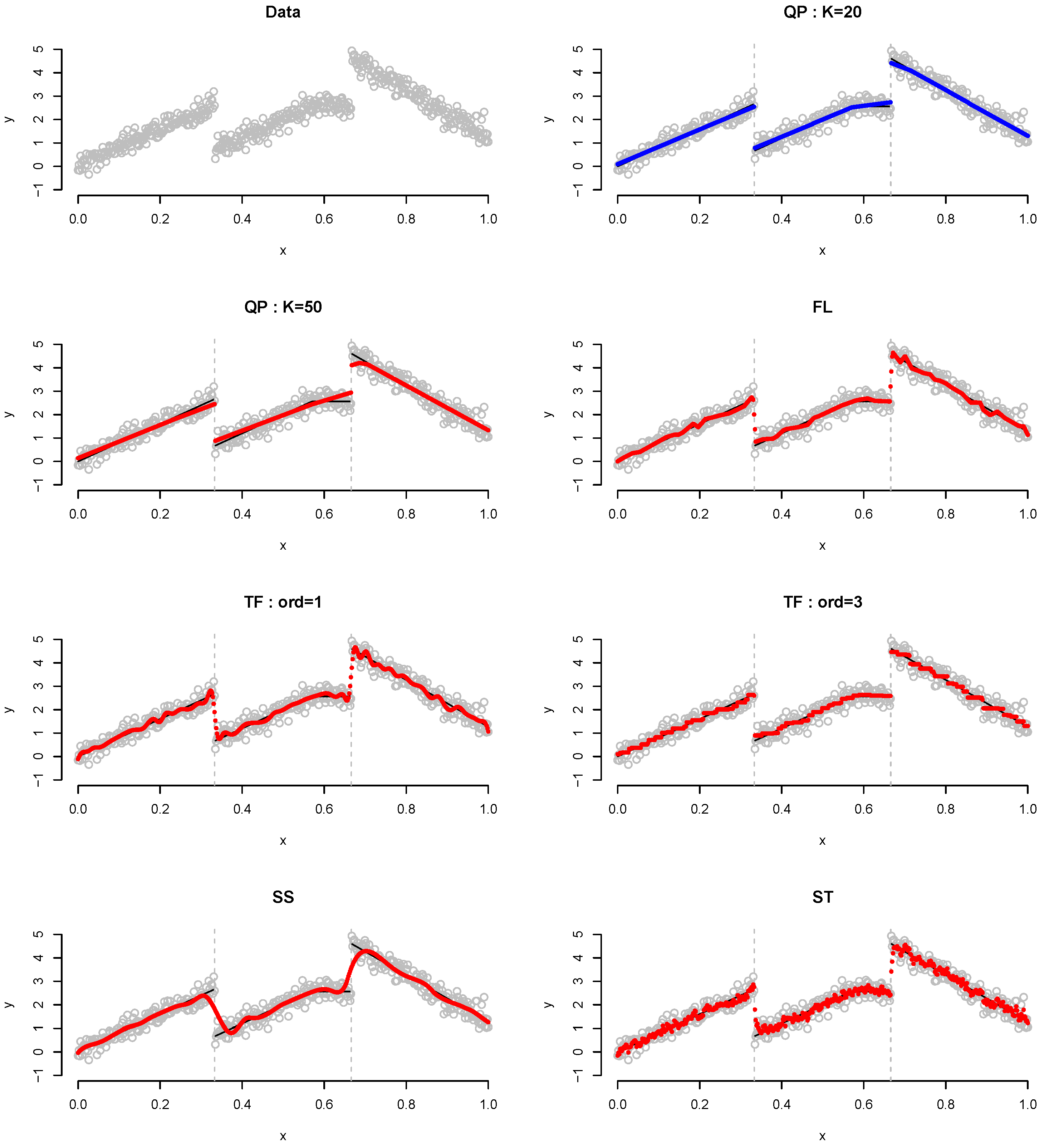
4.1. Simulation

In this section, we analyze the performance of the proposed method based on simulated examples. From model (1), we generate the predictor as n sequences in the range [ 0 , 1 ] . ε i is generated from N ( 0 , σ 2 ) for i = 1 , , n and σ is set 0.25 for all examples.
Next, we present three examples, as follows.
Example 1.
Piecewise linear function with a single change point
f ( x ) = 13 x i f . 333 0 x < 0.333 10 x + 3 i f 0.333 x 1
Example 2.
Piecewise linear function with two change points
f ( x ) = 8 x i f . 333 0 x < 0.333 8 x 2 i f 0.333 x < 0.570 2.56 i f 0.570 x < 0.666 10 x + 11.27 i f 0.666 x 1
Example 3.
Piecewise cubic function with a single change point
f ( x ) = 20 x 3 + 50 x 2 i f . 333 0 x < 0.333 12 x 2 + 15 i f 0.333 x 1
In Examples 1–2, a linear model with the jump(s) is considered. In Example 1, the true knot is 0.333, whereas they are 0.333 and 0.666 in Example 2. Example 3 is designed as a nonlinear function, where the true function is of quadratic and cubic form. Figure 2 shows the true functions of Examples 1–3.
We compare the proposed method with the fused lasso (FL) of Tibshirani et al. [17], the trend filtering (TF) of Kim et al. [25], the smoothing spline (SS) of Kim and Gu [26] and a fitting method for the structural model for a time series (ST) by Harvey [27].
The FL is a method that yields a solution path for the general fused lasso problem. The TF is the method of computing the solution path for the trend filtering problem of an arbitrary polynomial order. The SS is a method of fitting smoothing spline ANOVA models in Gaussian regression. The ST fits a structural model for a time series using the maximum likelihood. It is noteworthy that the FL, TF and SS estimators use nonparametric regression function estimation models. In particular, the TF and SS are function estimators based on linear combinations of spline basis functions, similar to ours. In addition, the FL is an estimator that specializes in change point detection as a zero-degree piecewise constant function.
The FL and TF estimators are provided in the genlasso package in R [28]. They require the use of cross-validation for parameter selection. In addition, the SS and ST can be used in R via the gss [29] and stats packages [30], respectively. To reduce the computational burden, we compute all the estimators using the default settings for each package.
We consider the mean squared error (MSE), mean absolute error (MAE) and maximum deviation (MXDV) criterion as loss functions that measure the discrepancy between the true function f and each function estimator f ^ . They are expressed as follows:
MSE f ^ = 1 n i = 1 n f ( x i ) f ^ ( x i ) 2 , MAE f ^ = 1 n i = 1 n f ( x i ) f ^ ( x i )
and MXDV f ^ = max 1 i n f ( x i ) f ^ ( x i ) .
Examples 1–2 are simulated based on d = 1 , whereas Example 3 is simulated based on d = 3 , with K = 20 and K = 50 , respectively. In addition, a simulation is performed by setting TF with orders 1 and 3 for linear and cubic functions, respectively. The simulation is repeated 100 times for each example based on sample sizes of 200, 300 and 500. Table 1, Table 2 and Table 3 show the experimental results of various scenarios for each of the examples.
As shown in Table 1, because QP not only can detect change points (or jumps), but can also fit piecewise polynomial regression, it demonstrates the best performance compared with the other methods. Comparing the QP results based on K, it is discovered that the best performance is obtained when K = 20 . Figure 3 shows the plot for the results of Example 1 when n = 500 . QP detects the change point and fits the linear regression accurately, particularly when K = 20 . Although the performances of FL and TF with order 1 improve in general as the sample size n increases, it cannot detect the change point. Herein, “cannot detect the change point” means that, around the true knot, the plot has point(s) alone or successive.
Table 2 lists the results of Example 2, which is involved the same slope, two jumps and no jump at x = 0.57 . It is observed that QP demonstrates the best performance when K = 20 , not K = 50 . Figure 4 shows the plot for Example 2 when n = 500 . QP detects the change point and fits the linear regression accurately, particularly when K = 20 . Although most performances of FL and TF with order 1 improve in general, as the sample size n increases, they cannot detect the change point. Herein, “cannot detect the change point” means that, around the true knot, the plot has point(s) alone or successive.
Table 3 lists the results of Example 3, which is involved one jump as well as quadratic and cubic forms. Similarly, the proposed QP estimator yieldes the best results. K = 20 yieldes the best results in terms of the MSE and MAE, whereas K = 50 in terms of the MXDV. Figure 5 shows the results of Example 3 for all methods when n = 500 . As shown, even when it do not fit the polynomial regression line well at K = 50 , it detects the point of change accurately at the true knot.
QP detects the change point and fits the linear regression accurately, particularly when K = 20 . Although the performances of the FL and TF with order 1 improve as the sample size n increases, they cannot detect the change point. Herein, “cannot detect the change point” means that, around the true knot, the plot has point(s) alone or successive.

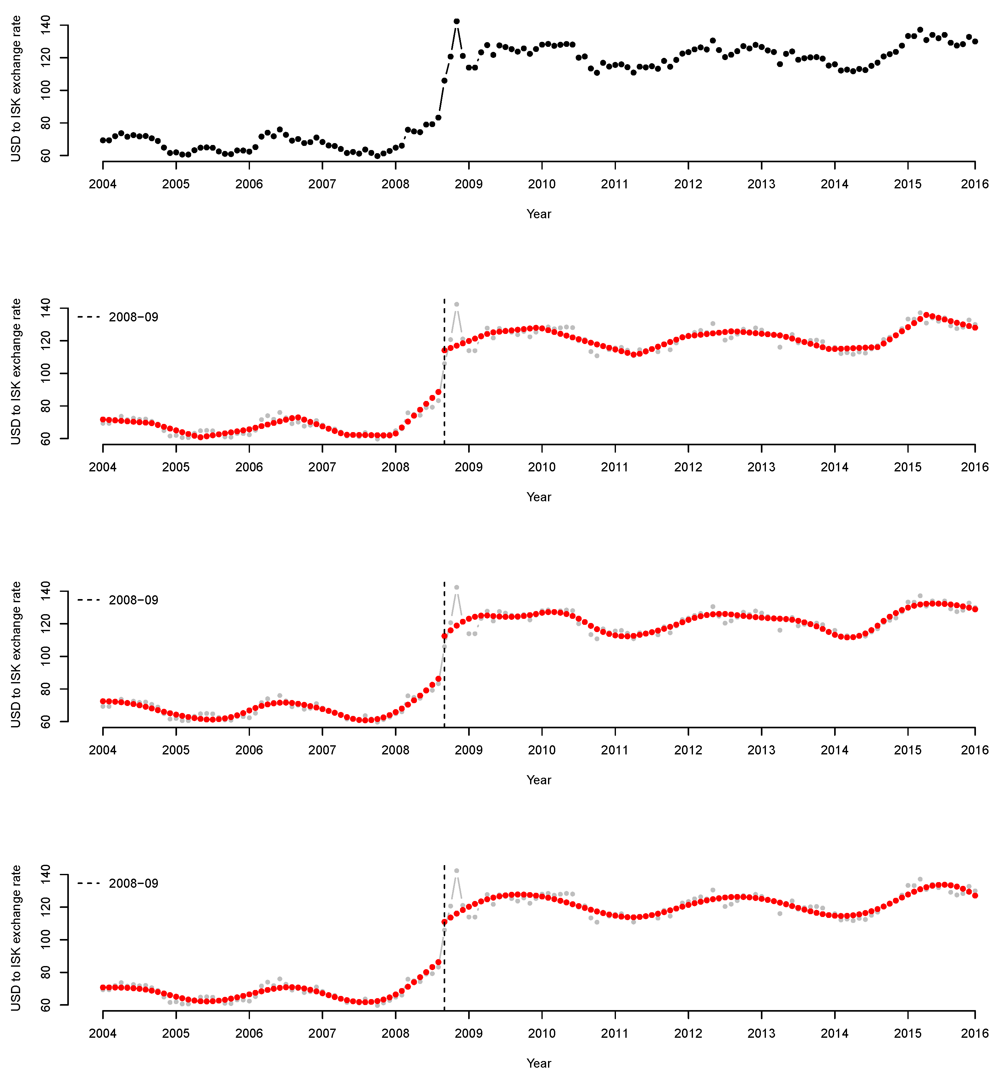
4.2. Real Data Analysis

The data obtained from Investing.com (last accessed date: 1 October 2021) the exchange rate change of the Icelandic króna (ISK) per US dollar (USD) from January 2004 to December 2015, measured as the monthly average.
The data contained 144 sets of observations associated with the subprime mortgage crisis, which occurred between 2007 and 2008. This crisis refers to a series of economic crises that began with the bankruptcy of the largest mortgage lenders in the United States and caused a credit crunch not only in the United States, but also in the international financial market. One of affected countries was Iceland, whose three largest banks were affected by the crisis in September 2008. To revive the economy, the Icelandic government has implemented various policies, including the nationalization of banks. Consequently, the ISK exchange rate per USD increased. In Figure 6, the top panel shows the starting point for the data. In January 2004, the observed value is 69.345; in March 2008, the observed value increases gradually to 75.805 and then increases significantly to 105.965 in September. In the last observation, performed in December 2016, a continuous increase of the value is observed (129.960).
Because the input variable is a date and not numeric data, 144 samples are equally spaced in the interval [0, 1] for the proposed QP implementation. A degree exceeding four can result in a more complicated interpretation and overfitting. Therefore, we apply d = 1 , 2 and 3.
Figure 6 shows the fitted results. The top panel of Figure 6 shows a scatterplot of the data. The remaining panels show the results of the QP model fitting when d = 1 , 2 and 3. It appears that the proposed MDSE based on the BIC detects a change point in September 2008 and fits the flow of the exchange rate well. Prior to 2008, no significant change is detected, but from January 2008, the exchange rate of ISK per USD increases gradually. Subsequently, beginning from September 2008, the exchange rate of ISK per USD increases significantly, as indicated by the vertical black dashed line in the figure (representing September 2008).

5. Conclusions

In this study, we develop a nonparametric regression function estimation method with change point detection. In order to provide a data-driven knot selection method, we consider elastic-net-type L 1 -norm penalty for the estimating regression function. Once we expressed the estimator with a linear combination of truncated power splines, the coefficients were estimated by minimizing a penalized residual sum of squares. A new coordinate descent algorithm and an algorithm based on quadratic programming are introduced to handle penalty terms determined by the regression coefficients. In the numerical analysis, we only use an algorithm based on quadratic programming because of the high computational cost of the coordinate descent algorithm when the number of knots increases. To verify the performance of the proposed estimator (MDSE), in the three simulations, we compared MDSE with four methods; the fused lasso (FL), trend filtering (TF), smoothing spline (SS) and structural model for a times series (ST). As a result, in all simulations, the MDSE detected the change point(s) and fitted linear and cubic trends of the piecewise polynomial well. Furthermore, we performed an actual data analysis about the sharp change in exchange rate of the Icelandic króna per US dollar in September 2008 caused by the subprime mortgage crisis in the United States between 2007 and 2008. In conclusion, MDSE can accurately detect September 2008, the time when a sharp increase in the exchange rate occurred, and can also represent the exchange rate trend before and after September 2008 well.
To improve the proposed coordinate descent algorithm, one may apply the B-spline basis and total variation penalty terms. The B-spline basis function is a numerically superior alternative to the truncated power basis. Because it has small supports, the predictor matrix is sparse and the information matrix is banded (chapter 1 and 8 of [31]). The B-spline-based total variation penalty term is a generalized lasso problem [32,33] that is difficult to implement, but affords high computational power. These approaches will be investigated in future studies.

Supplementary Materials

The following are available at https://www.mdpi.com/article/10.3390/axioms10040331/s1, The supplementary files contain a data set and R code to perform the proposed method described in the article (implemented by the software R version 4.0.2.).

Author Contributions

The authors contributed equally to this study; methodology, E.-J.L. (numerical framework) and J.-H.J. (modeling and defining estimator); implementation, E.-J.L. (CDA), J.-H.J. (QP); writing, E.-J.L. (numerical analysis), J.-H.J. (model and estimator). All authors have read and agreed to the published version of the manuscript.

Funding

This study was supported by the Basic Science Research Program through the National Research Foundation of Korea (NRF) funded by the Ministry of Education, Science and Technology (NRF-2020R1G1A1A01100869).

Institutional Review Board Statement

Not applicable.

Informed Consent Statement

Not applicable.

Data Availability Statement

Data are provided in the Supplementary Materials.

Acknowledgments

The authors wish to thank Jae-Kwon Oh for assistance with the numerical study.

Conflicts of Interest

The authors declare no conflict of interest.

References

  1. Tsybakov, A.B. Introduction to Nonparametric Estimation; Springer Science & Business Media: Berlin/Heidelberg, Germany, 2008. [Google Scholar]
  2. Fan, J.; Gijbels, I.; Hu, T.C.; Huang, L.S. A study of variable bandwidth selection for local polynomial regression. Stat. Sin. 1996, 6, 113–127. [Google Scholar]
  3. Efromovich, S. Nonparametric Curve Estimation: Methods, Theory, and Applications; Springer Science & Business Media: Berlin/Heidelberg, Germany, 2008. [Google Scholar]
  4. Green, P.J.; Silverman, B.W. Nonparametric Regression and Generalized Linear Models: A Roughness Penalty Approach; CRC Press: Boca Raton, FL, USA, 1993. [Google Scholar]
  5. Massopust, P. Interpolation and Approximation with Splines and Fractals; Oxford University Press, Inc.: Oxford, UK, 2010. [Google Scholar]
  6. James, G.; Witten, D.; Hastie, T.; Tibshirani, R. An introduction to Statistical Learning; Springer: Berlin/Heidelberg, Germany, 2013; Volume 112. [Google Scholar]
  7. Wright, S.J. Coordinate descent algorithms. Math. Program. 2015, 151, 3–34. [Google Scholar] [CrossRef]
  8. Tseng, P. Convergence of a block coordinate descent method for nondifferentiable minimization. J. Optim. Theory Appl. 2001, 109, 475–494. [Google Scholar] [CrossRef]
  9. Tibshirani, R. Regression shrinkage and selection via the lasso. J. R. Stat. Soc. Ser. (Methodol.) 1996, 58, 267–288. [Google Scholar] [CrossRef]
  10. Meier, L.; Van De Geer, S.; Bühlmann, P. The group lasso for logistic regression. J. R. Stat. Soc. Ser. (Stat. Methodol.) 2008, 70, 53–71. [Google Scholar] [CrossRef]
  11. Zou, H.; Hastie, T. Regularization and variable selection via the elastic net. J. R. Stat. Soc. Ser. (Stat. Methodol.) 2005, 67, 301–320. [Google Scholar] [CrossRef]
  12. Goldfarb, D.; Idnani, A. A numerically stable dual method for solving strictly convex quadratic programs. Math. Program. 1983, 27, 1–33. [Google Scholar] [CrossRef]
  13. Osborne, M.; Presnell, B.; Turlach, B. Knot selection for regression splines via the lasso. Comput. Sci. Stat. 1998, 30, 44–49. [Google Scholar]
  14. Leitenstorfer, F.; Tutz, G. Knot selection by boosting techniques. Comput. Stat. Data Anal. 2007, 51, 4605–4621. [Google Scholar] [CrossRef]
  15. Garton, N.; Niemi, J.; Carriquiry, A. Knot selection in sparse Gaussian processes. arXiv 2020, arXiv:2002.09538. [Google Scholar]
  16. Aminikhanghahi, S.; Cook, D.J. A survey of methods for time series change point detection. Knowl. Inf. Syst. 2017, 51, 339–367. [Google Scholar] [CrossRef] [PubMed]
  17. Tibshirani, R.; Saunders, M.; Rosset, S.; Zhu, J.; Knight, K. Sparsity and smoothness via the fused lasso. J. R. Stat. Soc. Ser. (Stat. Methodol.) 2005, 67, 91–108. [Google Scholar] [CrossRef]
  18. Turlach, B.A.; Weingessel, A. Quadprog: Functions to Solve Quadratic Programming Problems; R Package Version 1.5-8. 2019. Available online: https://cran.r-project.org/package=quadprog (accessed on 15 July 2021).
  19. Friedman, J.; Hastie, T.; Tibshirani, R. Regularization paths for generalized linear models via coordinate descent. J. Stat. Softw. 2010, 33, 1–22. [Google Scholar] [CrossRef] [PubMed]
  20. Jhong, J.H.; Koo, J.Y.; Lee, S.W. Penalized B-spline estimator for regression functions using total variation penalty. J. Stat. Plan. Inference 2017, 184, 77–93. [Google Scholar] [CrossRef]
  21. Bozdogan, H. Model selection and Akaike’s information criterion (AIC): The general theory and its analytical extensions. Psychometrika 1987, 52, 345–370. [Google Scholar] [CrossRef]
  22. Schwarz, G. Estimating the dimension of a model. Ann. Stat. 1978, 6, 461–464. [Google Scholar] [CrossRef]
  23. Luenberger, D.G.; Ye, Y. Linear and Nonlinear Programming; Springer: Berlin/Heidelberg, Germany, 1984; Volume 2. [Google Scholar]
  24. Rockafellar, R.T. Convex Analysis; Princeton University Press: Princeton, NJ, USA, 2015. [Google Scholar]
  25. Kim, S.J.; Koh, K.; Boyd, S.; Gorinevsky, D. 1 trend filtering. SIAM Rev. 2009, 51, 339–360. [Google Scholar] [CrossRef]
  26. Kim, Y.J.; Gu, C. Smoothing spline Gaussian regression: More scalable computation via efficient approximation. J. R. Stat. Soc. Ser. (Stat. Methodol.) 2004, 66, 337–356. [Google Scholar] [CrossRef]
  27. Harvey, A.C. Forecasting, Structural Time Series Models and the Kalman Filter; Cambridge University Press: Cambridge, UK, 1990. [Google Scholar]
  28. Arnold, T.B.; Tibshirani, R.J. Efficient implementations of the generalized lasso dual path algorithm. J. Comput. Graph. Stat. 2016, 25, 1–27. [Google Scholar] [CrossRef]
  29. Gu, C. Smoothing spline ANOVA models: R package gss. J. Stat. Softw. 2014, 58, 1–25. [Google Scholar] [CrossRef]
  30. R Core Team. R: A Language and Environment for Statistical Computing; R Core Team: Vienna, Austria, 2021. [Google Scholar]
  31. De Boor, C.; De Boor, C. A Practical Guide to Splines; Springer: New York, NY, USA, 1978; Volume 27. [Google Scholar] [CrossRef]
  32. Roth, V. The generalized LASSO. IEEE Trans. Neural Netw. 2004, 15, 16–28. [Google Scholar] [CrossRef] [PubMed]
  33. Tibshirani, R.J.; Taylor, J. The solution path of the generalized lasso. Ann. Stat. 2011, 39, 1335–1371. [Google Scholar] [CrossRef]
Figure 1. Plot showing comparison between CDA and QP. Red circles and blue triangles represent CDA and QP fitted values, respectively.
Axioms 10 00331 g001
Figure 2. Plot showing true function of Examples 1–3. Top-left panel is for Example 1, which has a true knot of 0.333. Top-right panel is for Example 2, which has two true knots of 0.333 and 0.666. Bottom-left panel is for Example 3, which exhibits a nonlinear form with a true knot of 0.333.
Axioms 10 00331 g002
Figure 3. Plot for Example 1 when n = 500 . Gray dots, data points; blue dots, best-fitted values; red dots, remaining fitted values.
Axioms 10 00331 g003
Figure 4. Plot for Example 2 when n = 500 . Gray dots, data points; blue dots, best-fitted values; red dots, remaining fitted values.
Axioms 10 00331 g004
Figure 5. Plot for Example 3 when n = 500 . Gray dots, data points; blue dots, best-fitted values; red dots, remaining fitted values.
Axioms 10 00331 g005
Figure 6. (Top) USD to ISK exchange rate data. The x-axis corresponds to the input variable in a year, i.e., each month from January 2004 to December 2015. The y-axis shows the monthly average of the ISK exchange rate against USD for each month. First panel in the middle, fit result when d = 1 (linear); second panel in the middle, fit result when d = 2 (quadratic); bottom panel, fit result when d = 3 (cubic). The bottom three panels are indicated by a vertical black dashed line between 2008 and 2009, as well as red points. The dashed line indicates the change point, whereas the red dots indicate the fitted results.
Axioms 10 00331 g006
Table 1. Average ( × 100 ) of each criterion over 100 trials of QP, FL, TF, SS and ST for Example 1 (for sample size n = 200, 300 and 500; standard error in parentheses). Bold text represents smallest criterion for each scenario.
n QP (K = 20)QP (K = 50)FLTF (ord = 1)TF (ord = 3)SSST
200MSE0.520.801.721.963.549.474.55
( 3 × 10 3 )( 6 × 10 3 )( 3 × 10 3 )( 7 × 10 3 )( 8 × 10 3 )( 3 × 10 2 )( 9 × 10 3 )
MAE4.275.3510.418.4511.7713.1616.18
( 1 × 10 2 )( 2 × 10 2 )( 1 × 10 2 )( 1 × 10 2 )( 2 × 10 2 )( 2 × 10 2 )( 4 × 10 3 )
MXDV37.7049.6739.71102.70133.93217.82117.69
( 2 × 10 1 )( 3 × 10 1 )( 7 × 10 2 )( 4 × 10 1 )( 3 × 10 1 )( 2 × 10 1 )( 2 × 10 2 )
300MSE0.220.400.941.112.117.852.91
( 1 × 10 3 )( 4 × 10 3 )( 2 × 10 3 )( 4 × 10 3 )( 4 × 10 3 )( 3 × 10 2 )( 7 × 10 3 )
MAE2.743.787.726.158.6610.7012.76
( 8 × 10 3 )( 1 × 10 2 )( 7 × 10 3 )( 1 × 10 2 )( 1 × 10 2 )( 2 × 10 2 ( 3 × 10 3 )
MXDV25.8437.0229.9095.21133.34222.44120.09
( 1 × 10 1 )( 2 × 10 1 )( 6 × 10 2 )( 3 × 10 2 )( 3 × 10 2 )( 1 × 10 2 )( 2 × 10 2 )
500MSE0.130.220.650.924.577.072.55
( 9 × 10 4 )( 2 × 10 3 )( 1 × 10 3 )( 2 × 10 3 )( 7 × 10 3 )( 2 × 10 2 )( 5 × 10 3 )
MAE2.012.706.445.436.919.4311.62
( 5 × 10 3 )( 1 × 10 2 )( 4 × 10 3 )( 8 × 10 3 )( 5 × 10 3 )( 2 × 10 2 )( 2 × 10 3 )
MXDV19.8428.9526.03113.64218.35232.12159.22
( 1 × 10 1 )( 2 × 10 1 )( 5 × 10 2 )( 3 × 10 1 )( 6 × 10 2 )( 1 × 10 1 )( 2 × 10 1 )
Table 2. Average ( × 100 ) of each criterion over 100 trials of QP, FL, TF, SS and ST for Example 2 (for sample sizes n = 200, 300 and 500; standard error in parentheses). The bold text represents the smallest criterion for each scenario.
n QP (K = 20)QP (K = 50)FLTF (ord = 1)TF (ord = 3)SSST
200MSE0.621.391.512.102.894.443.51
( 3 × 10 3 )( 1 × 10 2 )( 3 × 10 3 )( 4 × 10 3 )( 8 × 10 3 )( 9 × 10 3 )( 8 × 10 3 )
MAE5.658.329.659.2011.4611.9313.96
( 1 × 10 2 )( 3 × 10 2 )( 1 × 10 2 )( 2 × 10 2 )( 2 × 10 2 )( 1 × 10 2 )( 4 × 10 3 )
MXDV28.5039.8838.9283.5286.71100.9093.29
( 1 × 10 1 )( 2 × 10 1 )( 8 × 10 2 )( 1 × 10 1 )( 1 × 10 1 )( 6 × 10 2 )( 1 × 10 1 )
300MSE0.430.581.131.642.193.823.05
( 2 × 10 3 )( 4 × 10 3 )( 2 × 10 3 )( 3 × 10 3 )( 3 × 10 3 )( 6 × 10 3 )( 9 × 10 3 )
MAE4.725.508.377.879.7210.5312.67
( 1 × 10 2 )( 1 × 10 2 )( 8 × 10 3 )( 1 × 10 2 )( 1 × 10 2 )( 1 × 10 2 )( 4 × 10 3 )
MXDV25.3329.6636.3086.7189.47103.02107.01
( 9 × 10 2 )( 1 × 10 1 )( 1 × 10 1 )( 1 × 10 1 )( 1 × 10 1 )( 5 × 10 2 )( 1 × 10 2 )
500MSE0.250.630.761.201.663.212.49
( 1 × 10 3 )( 5 × 10 3 )( 1 × 10 3 )( 1 × 10 3 )( 1 × 10 3 )( 6 × 10 3 )( 6 × 10 3 )
MAE3.525.216.876.547.769.0911.23
( 8 × 10 3 )( 2 × 10 2 )( 6 × 10 3 )( 1 × 10 2 )( 9 × 10 3 )( 1 × 10 2 )( 2 × 10 3 )
MXDV20.3332.8932.4291.1296.79105.51122.67
( 9 × 10 2 )( 1 × 10 1 )( 1 × 10 1 )( 8 × 10 2 )( 5 × 10 2 )( 6 × 10 2 )( 1 × 10 1 )
Table 3. Average ( × 100 ) of each criterion over 100 trials of QP, FL, TF, SS and ST for Example 3 (for sample sizes n = 200, 300 and 500; standard error in parentheses). Bold text represents smallest criterion for each scenario.
n QP (K = 20)QP (K = 50)FLTF (ord = 1)TF (ord = 3)SSST
200MSE0.951.972.301.774.8126.965.53
( 6 × 10 3 )( 3 × 10 3 )( 6 × 10 3 )( 5 × 10 3 )( 1 × 10 2 )( 1 × 10 1 )( 1 × 10 2 )
MAE6.7311.1111.908.6212.5918.8318.58
( 2 × 10 2 )( 9 × 10 3 )( 1 × 10 2 )( 2 × 10 2 )( 2 × 10 2 )( 4 × 10 2 )( 6 × 10 3 )
MXDV50.0641.9546.8591.63165.54382.1481.19
( 1 × 10 1 )( 6 × 10 2 )( 9 × 10 2 )( 3 × 10 1 )( 6 × 10 1 )( 3 × 10 1 )( 2 × 10 1 )
300MSE0.631.461.651.573.9723.485.20
( 2 × 10 3 )( 2 × 10 3 )( 2 × 10 3 )( 3 × 10 3 )( 6 × 10 3 )( 8 × 10 2 )( 9 × 10 3 )
MAE5.469.5210.107.6911.2016.7017.69
( 9 × 10 3 )( 8 × 10 3 )( 7 × 10 3 )( 1 × 10 2 )( 1 × 10 2 )( 4 × 10 2 )( 5 × 10 3 )
MXDV47.3238.7242.29113.08191.36395.16119.95
( 1 × 10 1 )( 6 × 10 2 )( 8 × 10 2 )( 3 × 10 1 )( 4 × 10 1 )( 2 × 10 1 )( 3 × 10 1 )
500MSE0.501.021.171.5015.9021.604.79
( 1 × 10 3 )( 2 × 10 3 )( 1 × 10 3 )( 7 × 10 3 )( 2 × 10 2 )( 8 × 10 2 )( 7 × 10 3 )
MAE4.567.798.506.9611.2315.1716.37
( 7 × 10 3 )( 9 × 10 3 )( 5 × 10 3 )( 9 × 10 3 )( 9 × 10 3 )( 4 × 10 2 )( 4 × 10 3 )
MXDV47.8738.8539.65146.05390.08407.96193.31
( 8 × 10 2 )( 6 × 10 2 )( 9 × 10 2 )( 5 × 10 1 )( 8 × 10 2 )( 2 × 10 1 )( 3 × 10 1 )
Publisher’s Note: MDPI stays neutral with regard to jurisdictional claims in published maps and institutional affiliations.

